Article

Spatiotemporal Variation in NDVI in the Sunkoshi River Watershed During 2000–2021 and Its Response to Climate Factors and Soil Moisture

by
Zhipeng Jian
1,
Qinli Yang
1,*,
Junming Shao
2,
Guoqing Wang
3 and
Vishnu Prasad Pandey
4,5
1
School of Resources and Environment, University of Electronic Science and Technology of China, Chengdu 611731, China
2
School of Computer Science and Engineering, University of Electronic Science and Technology of China, Chengdu 611731, China
3
State Key Laboratory of Hydrology-Water Resources and Hydraulic Engineering, Nanjing Hydraulic Research Institute, Nanjing 210029, China
4
Department of Civil Engineering, Pulchowk Campus, Institute of Engineering, Tribhuvan University, Lalitpur 44700, Nepal
5
Center for Water Resources Studies, Institute of Engineering, Tribhuvan University, Lalitpur 44700, Nepal
*
Author to whom correspondence should be addressed.
Water 2025, 17(15), 2232; https://doi.org/10.3390/w17152232
Submission received: 4 June 2025 / Revised: 20 July 2025 / Accepted: 21 July 2025 / Published: 26 July 2025
(This article belongs to the Section Hydrology)

Abstract

Given that the Sunkoshi River watershed (located in the southern foot of the Himalayas) is sensitive to climate change and its mountain ecosystem provides important services, we aim to evaluate its spatial and temporal variation patterns of vegetation, represented by the Normalized Difference Vegetation Index (NDVI), during 2000–2021 and identify the dominant driving factors of vegetation change. Based on the NDVI dataset (MOD13A1), we used the simple linear trend model, seasonal and trend decomposition using loess (STL) method, and Mann–Kendall test to investigate the spatiotemporal variation features of NDVI during 2000–2021 on multiple scales (annual, seasonal, monthly). We used the partial correlation coefficient (PCC) to quantify the response of the NDVI to land surface temperature (LST), precipitation, humidity, and soil moisture. The results indicate that the annual NDVI in 52.6% of the study area (with elevation of 1–3 km) increased significantly, while 0.9% of the study area (due to urbanization) degraded significantly during 2000–2021. Daytime LST dominates NDVI changes on spring, summer, and winter scales, while precipitation, soil moisture, and nighttime LST are the primary impact factors on annual NDVI changes. After removing the influence of soil moisture, the contributions of climate factors to NDVI change are enhanced. Precipitation shows a 3-month lag effect and a 5-month cumulative effect on the NDVI; both daytime LST and soil moisture have a 4-month lag effect on the NDVI; and humidity exhibits a 2-month cumulative effect on the NDVI. Overall, the study area turned green during 2000–2021. The dominant driving factors of NDVI change may vary on different time scales. The findings will be beneficial for climate change impact assessment on the regional eco-environment, and for integrated watershed management.

1. Introduction

As the main component of the terrestrial ecosystem, vegetation plays essential roles in terrestrial carbon cycles, energy exchange, and the water balance at various spatial and temporal scales [1]. Both the climate and soil moisture exert influences on vegetation. Climate impacts vegetation directly and significantly via the biophysical processes of plant photosynthesis, respiration, and evapotranspiration [2], while soil moisture impacts vegetation by limiting water and the energy provision [3]. Driven by the spatiotemporal changes in climate and soil moisture, correspondingly, the vegetation index (e.g., NDVI) often exhibits certain spatiotemporal variation patterns, particularly for the areas (such as the Himalayas, Qinghai-Tibet Plateau) where the vegetation is sensitive to changes in environmental factors (such as temperature and precipitation). Moreover, the IPCC AR 6 report indicates that extreme weather and climatic events will become more frequent [4], which would impact vegetation significantly. Furthermore, the primary driving factors of vegetation change may differ in time and space. Identifying the key factors may shed light on the mechanisms of the response of terrestrial carbon storage to climate variability. Therefore, studying the spatiotemporal variation characteristics of vegetation and its response to climate factors and soil moisture is of great importance for regional ecosystem assessment, carbon storage quantification, and understanding the soil moisture–vegetation–climate interaction mechanisms.
Numerous studies on the response of vegetation to climate change have been conducted [5,6]. In previous studies, air temperature and precipitation observed at meteorological stations were often used to represent climate change [7,8], and NDVI is commonly regarded as a good indicator of vegetation growth dynamics [9]. Although air temperature and precipitation data measured at meteorological stations have high accuracy, their spatial representation is relatively low, especially for areas where meteorological stations are limited and sparsely distributed [10]. Therefore, satellite-based land surface temperature (LST) data (e.g., MOD11A2), precipitation data (e.g., Integrated Multi-satellite Retrievals for Global Precipitation Measurement (IMERG)), and humidity (e.g., MOD07) provide valuable data alternatives. Furthermore, the daily mean temperature was often used in previous studies, but few studies have distinguished the effects of daytime and nighttime temperature on vegetation [11]. In fact, the daytime temperature strongly affects the diurnal plant photosynthesis, and the nighttime temperature greatly influences nocturnal plant respiration [12]. Wen et al. [13] indicated that the impact of daytime and nighttime temperatures on the NDVI has important implications for climate–vegetation models, meaning that the impacts of the daytime LST and nighttime LST on vegetation need to be distinguished. Moreover, previous studies mostly used correlation coefficients to quantify the relationships between the NDVI and impact factors [14,15], which ignores correlations among different impact factors. Instead, partial correlation analysis is more appropriate, as it accounts for the correlations among different impact factors.
Soil moisture, as a straightforward index that reflects the amount of water available to plants [16], is another major factor influencing vegetation [3]. However, most works focus on the influence of vegetation on soil moisture, while they seldom pay attention to the influence of soil moisture on vegetation. For instance, Mohanty and Skaggs [17] indicated that the vegetation type, density, and uniformity are among the associated features that contribute to soil moisture variation at different space and time scales. Yang et al. [18] reported that where the vegetation density is high, the soil moisture is low. And the studies by Vreugdenhil et al. [19] demonstrated that vegetation parameters play an important role in estimating soil moisture. However, Nandintsetseg et al. [20] presented findings where the NDVI showed a strong correlation with soil moisture (r = 0.91) in the Northern Hemisphere during 1982–2005. Li et al. [21] implied that vegetation’s sensitivity to soil moisture significantly increased in many semi-arid and arid regions from 1982 to 2017. Hence, greater efforts are needed to explore the response of vegetation to soil moisture.
The Sunkoshi River watershed (SKRW), is a sub-region of Koshi River watershed (KRW), located in the southern foothills of the Himalayas, sensitive to climate change [22]. The SKRW has complex topography and rich vegetation types ranging from broad-leaved forests to grasslands. Certain studies on vegetation variation in the KRW have been conducted; however, consistent results of primary driving factors to vegetation change have not been achieved. For instance, Zhang et al. [23] analyzed spatiotemporal patterns of vegetation growth during 1982–2006 in the KRW and found the spatial patterns of vegetation varied and were significantly affected by temperature or precipitation over different periods. Wu et al. [24] investigated the spatiotemporal variations in vegetation in the KRW from 2000 to 2018, and revealed that there was no significant positive correlation between the increase in NDVI and precipitation. At present, the response of vegetation to climate change and soil moisture in the SKRW is still unclear. Therefore, this study aims to evaluate the spatial and temporal variations of vegetation in the Sunkoshi River watershed from 2000 to 2021, and to identify the dominant driving factors of vegetation change at multiple temporal scales.

2. Materials and Methods
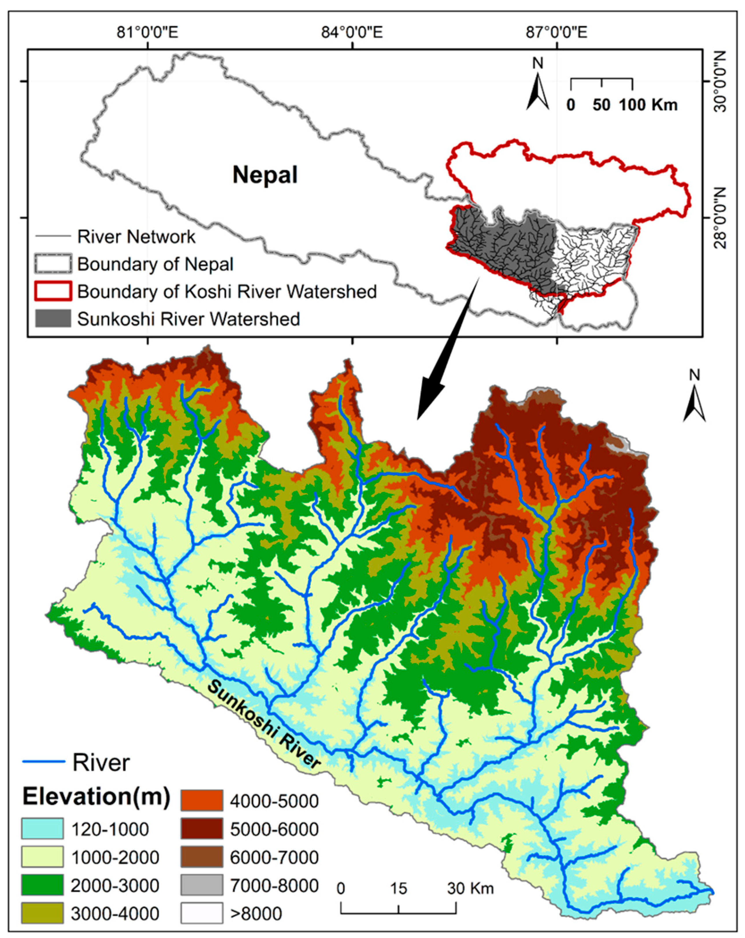
2.1. Study Area

We take the Sunkoshi River watershed (SKRW; 26°37′–28°32′ N, 85°43′–86°18′ E; Figure 1) as the study area. The size of the watershed is 14,745 km2, accounting for about 1/10 of Nepal’s land area. The SKRW has diverse vegetation types. Evergreen forests are predominant in the northern high-altitude regions, whereas grasslands and savanna are primarily distributed across the central and southern lowland areas. Croplands are mainly concentrated in the middle and lower reaches of the watershed. The elevation of the watershed varies significantly, ranging from 120 m to 8755 m above sea level. Due to the large elevation gradient, vegetation in the study area has a clear vertical zonation [25].
Monthly mean temperature ranges from 32.4–34.1 °C in summer to 9.1–11.3 °C in winter. Impacted by the South Asian monsoon climate, the annual mean precipitation is 1400 mm, 80% of which is concentrated in the period of June–September.

2.2. Data Sources

Compared with the NDVI data derived from the Advanced Very High-Resolution Radiometer (AVHRR), NDVI data derived from Moderate Resolution Imaging Spectroradiometer (MODIS) satellite imagery is particularly suitable for monitoring the dynamics of vegetation coverage at a regional scale due to their higher spatial resolution (500 m for MODIS vs. 1 km for AVHRR) [26,27]. Meanwhile, MODIS LST product and MOD07 humidity product agreed well with the ground LST [28,29,30]. Therefore, three MODIS land products, namely Terra 16-Day Vegetation Indices L3 (MOD13A1), Terra 8-Day Land Surface Temperature/Emissivity (MOD11A2), and MODIS/Terra Temperature and Water Vapor Profiles 5-Min L2 Swath 5 km (MOD07) are selected as data sources in this study.
The Global Precipitation Measurement (GPM) mission is an advanced successor to the Tropical Rainfall Measuring Mission (TRMM). In contrast to TRMM, GPM improves instruments (such as the Dual-frequency Precipitation Radar (DPR)) and provides precipitation measurements with higher spatial resolution (0.1°), higher temporal resolution (as frequent as half-hourly to every three hours), and a wider coverage range (60° S–60° N) [31,32]. Studies indicate that GPM provides more accurate and frequent measurements of daily rainfall accumulation and spatial rainfall patterns, especially during the pre-monsoon and monsoon seasons [33,34,35]. The Advanced Microwave Scanning Radiometer 2 (AMSR2) is a passive microwave sensor onboard the Global Change Observation Mission 1-Water (GCOM-W1) satellite that was launched by the Japan Aerospace Exploration Agency (JAXA) in May 2012. Kim et al. [36] pointed out that Bias and RMSE of the LPRM algorithm used for AMSR2 are generally smaller than those of JAXA algorithm when generating soil moisture product. Thus, precipitation data from GPM and soil moisture data from AMSR2/GCOM-W1 (LPRM) are selected as data sources in this study. Digital Elevation Model (DEM) data is downloaded from the Geospatial Data Cloud website. More details about these datasets are listed in Table 1. All images downloaded were mosaicked and re-projected to Albers.

2.3. Data Preprocess

Firstly, all datasets are converted from different formats into a uniform raster format. Since the nearest neighbor method does not introduce new or interpolated values but preserves the original data, the accuracy and uncertainty of the resampled datasets are inherited from the original data sources and there is no additional interpolation error introduced during the resampling process [37,38]. Therefore, to facilitate subsequent analysis and retain the accuracy of the original data, the nearest neighbor interpolation method, widely used in remote sensing and vegetation studies [39,40,41,42], is selected to resample all raster data to datasets with a spatial resolution of 500 m. Furthermore, to analyze NDVI variation and its response to climatic factors and soil moisture at different scales, datasets on monthly, seasonal and annual scales are reconstructed, respectively.
Monthly NDVI data was generated by taking the maximum composite data of two NDVI images in each month. Seasonal and annual NDVI datasets were generated by taking the average of monthly data in each season and each year, respectively. In this study, according to the monsoon and meteorological data analysis, March–May is regarded as spring, June–September is regarded as summer, October–November is regarded as autumn, and December–February in the next year is regarded as winter, and May–October is defined as the growing season [24,42]. Similarly, monthly, seasonal and annual datasets of other impact factors (LST, precipitation, humidity, and soil moisture) can be generated.
  • Simple linear trend (SLT) model
To analyze the trend of NDVI, the simple linear trend (SLT) model (Equation (1)) is applied, which has been proven to be an effective and widely used method for vegetation variation analysis [43,44,45,46].
s l o p e = n i = 1 n i NDVI i ( i = 1 n i ) ( i = 1 n NDVI i ) n i = 1 n i 2 ( i = 1 n i ) 2
where NDVIi represents the NDVI value at the time stamp i, and i is the time index of the NDVI sequence.
To index the spatial characteristics of NDVI trend, SLT analysis is performed on each pixel. In addition, a statistical hypothesis test is calculated to test the significance of the NDVI change on each pixel [45,47].
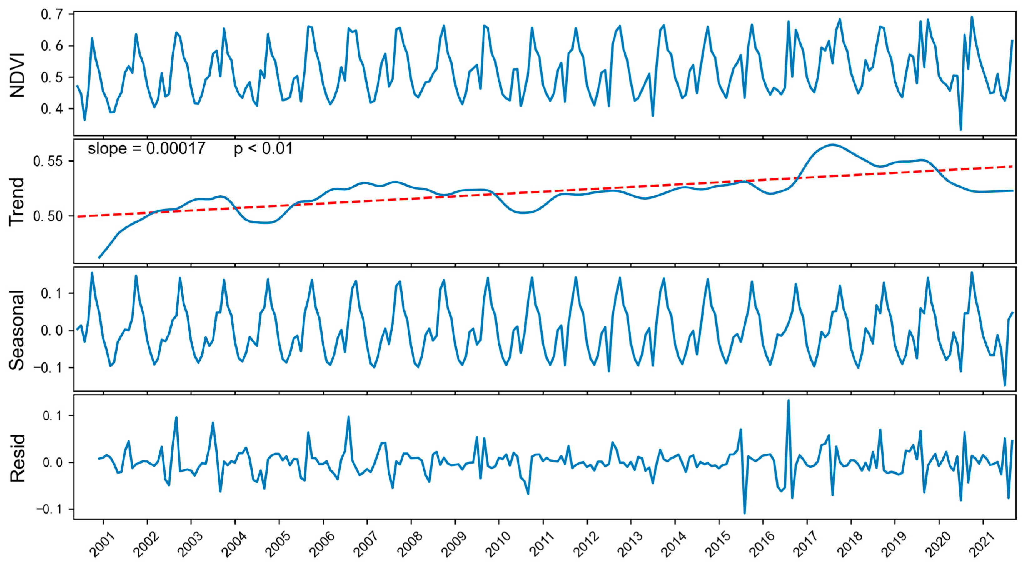
  • Seasonal and trend decomposition using loess (STL) method
The Seasonal and Trend decomposition using Loess (STL) algorithm [48] is a robust method of time series decomposition widely used in environmental analyses. Its basic idea is to decompose the original time series ( X v ) into three components: trend ( T v ), seasonal ( S v ), and remainder ( R v ).
X v = T v + S v + R v
The trend component is the low-frequency component of the data series, representing the trend and direction of change; the seasonal component is the high-frequency component of the data series, representing the regular change of the data over time, usually with a fixed period and amplitude; and the residual component represents the noise in the data series. In this study, the trend component of the NDVI data series decomposed by STL is further used for trend analysis of NDVI.
  • Mann–Kendall test
Mann–Kendall (MK) test [49,50] is a nonparametric statistical test for determination of trends in time series data. The MK test is given below:
S = i = 1 n 1 j = i + 1 n sgn ( x j x i )
sgn ( x i x j ) = + 1 i f   x i x j > 0   0 i f   x i x j = 0 1 i f   x i x j < 0
where n refers to the data length of the time series, and xi and xj are the data at time stamps i and j, respectively. When n >> 10, the statistic S approximately equals the standard normal test statistic (Z) value, which can be used to test the trend as follows:
Z = S 1 V a r ( s ) i f   S > 0         0 i f   S = 0 S + 1 V a r ( s ) i f   S < 0
V a r ( S ) = n ( n 1 ) ( 2 n + 5 ) i = 1 m t i ( t i 1 ) ( 2 t i + 5 ) 18
where n refers to the data length of the time series, m is the number of repeated datasets in the time series data and t denotes the repeated data values in the i t h group. When Z > Z 1 α / 2 , the null hypothesis can be rejected, which means the existence of a significant trend in the data. When Z < Z 1 α / 2 , the null hypothesis of trend will be accepted. In this study, α = 0.01 and α = 0.05 are defined as the given significance levels, and Z 1 α / 2 equals 2.576 and 1.96, respectively.
  • Partial correlation analysis
Partial correlation analysis is a method for quantifying the intrinsic relationship between two continuous variables, while statistically controlling for the effects of one or more other continuous variables [51,52]. In this study, in order to evaluate the correlation between NDVI and one specific impact factor while excluding the influences of other impact factors, partial correlation analysis is selected. The partial correlation coefficient (PCC) ranges from −1 to 1, which statistically represents a perfect negative relationship to a perfect positive correlation. The PCC value of 0 indicates NDVI has no correlation with the impact factor.
The first-order partial correlation coefficient and the second-order partial correlation coefficient are shown in (Equations (7)–(9)), respectively.
r i j h = r i j r i j r j h ( 1 r i h 2 ) ( 1 r j h 2 )
where r i j h is the partial correlation coefficient between i and j after excluding the influence of h; r i j is the simple correlation coefficient of i and j; r i h is the simple correlation coefficient of i and h; r j h is the simple correlation coefficient of j and h.
r i j h m = r i j h r i m h r j m h ( 1 r i m h 2 ) ( 1 r j m h 2 )
where r i j h m is the partial correlation coefficient between i and j after excluding the influences of h and m; r i j h is the partial correlation coefficient between i and j after excluding the influence of h; r i m h is the partial correlation coefficient between i and m after excluding the influence of h; r j m h is the partial correlation coefficient between j and m after excluding the influence of h.
r i j h m n = r i j h m r i n h m r j n h n ( 1 r i n h m 2 ) ( 1 r j n h m 2 )
where r i j h m n is the partial correlation coefficient between i and j after excluding the influences of h, m and n; r i j h m is the partial correlation coefficient between i and j after excluding the influences of h and m; r i n h m is the partial correlation coefficient between i and n after excluding the influences of h and m; r j n h m is the partial correlation coefficient between j and n after excluding the influences of h and m.
The partial correlation analysis among NDVI and impact factors are investigated at different spatial scales (pixel and watershed) and time scales (monthly, seasonal and annual).

3. Results

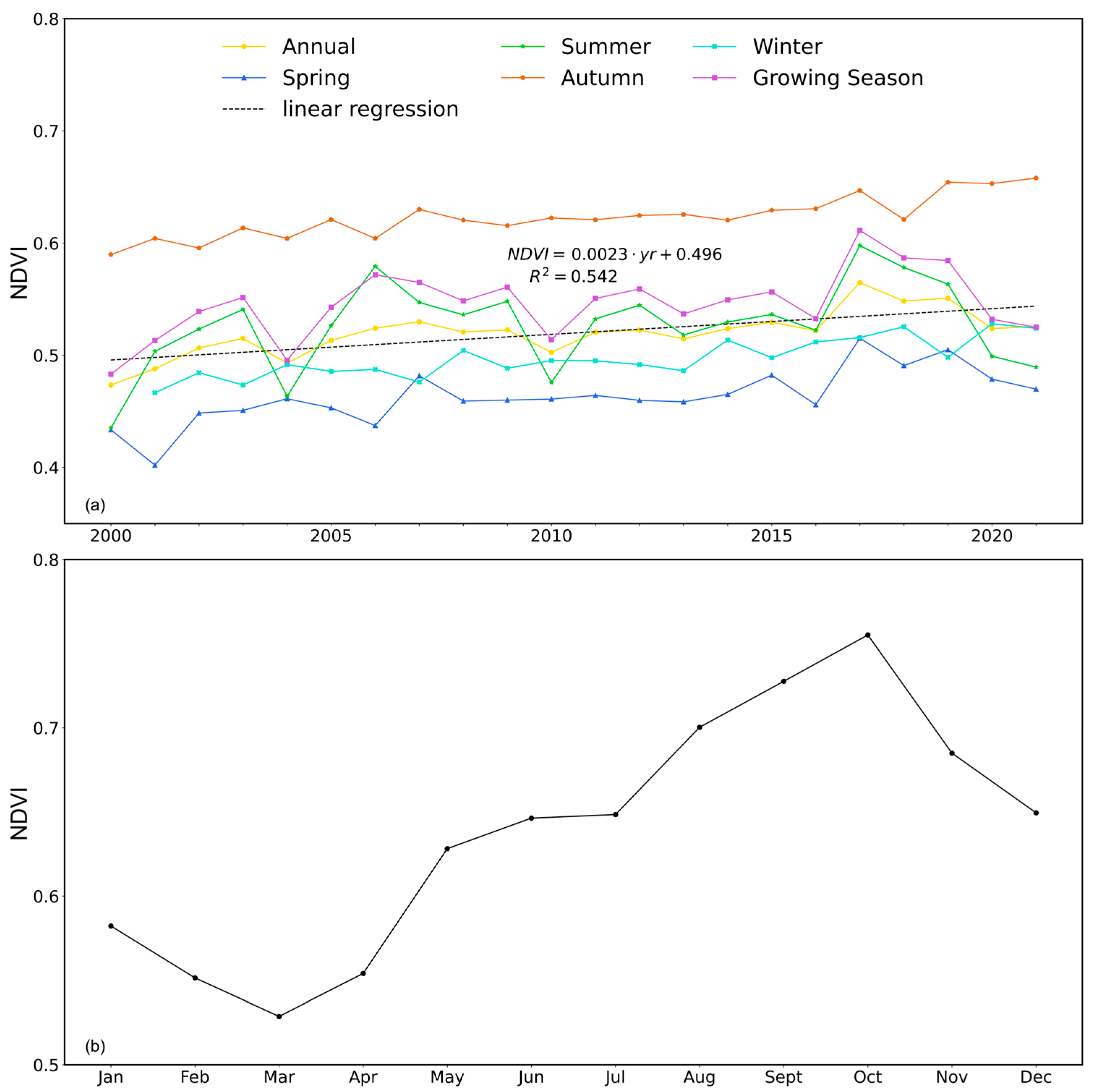
3.1. Temporal Variation Characteristics of Vegetation in the Watershed

To investigate the trend of vegetation in the study area, two widely used methods (simple linear trend (SLT) model and MK test) are selected and applied on NDVI data series. Figure 2a displays the inter-annual and intra-annual changes of NDVI at different time scales during 2000–2021, and Table 2 lists the corresponding change rates of NDVI based on the SLT model. In general, NDVI at both seasonal and annual scales show significant increase trends except for NDVI in summer. Annual NDVI increased significantly (p < 0.01) with a magnitude of 0.0023/year, which is consistent with the previous study by Wu et al. [24]. In terms of intra-annual change of NDVI, Figure 2b presents the monthly mean NDVI during 2000–2021 in the SKRW. It indicates NDVI reached the lowest value (0.529) in March, and then increased up to the highest value of 0.755 in October.
In contrast, Figure 3 shows the decomposition results of NDVI data series by using the STL method and the result of MK trend test on the trend component of NDVI. It indicates a significant increasing trend of NDVI, which is consistent with the result based on the SLT model. The seasonal component shows an obvious seasonality in NDVI series and NDVI reaches a peak in October annually, which is consistent with findings demonstrated in Figure 2b.

3.2. Spatial Variation Characteristics of Vegetation in the Watershed

The spatial variations of annual and seasonal NDVI during 2000–2021 are illustrated in Figure 4. Specifically, Figure 4a–f present distribution of change rate of NDVI at spring, summer, autumn, winter, growing season and annual scales, respectively. Figure 4g–l display the distribution of NDVI trend types with statistical significance at spring, summer, autumn, winter, growing season, and annual scales, respectively. The trend types include degradation with high significance (p < 0.01, red block), degradation with weak significance (p < 0.05, pink block), non-significant change (p > 0.05, orange block), improvement with weak significance (p < 0.05, green block), and improvement with high significance (p < 0.01, dark green block). It can be found that vegetation change shows high spatial heterogeneity.
Correspondingly, Table 3 summarizes the statistical information of different trend types of NDVI. In general, change patterns of NDVI in the study area show large spatial and temporal heterogeneity and a greening (improvement) trend dominates the whole watershed. Specifically, areas with annual improved NDVI account for 90.9%, of which 52.6% is significantly improved (S > 0, p < 0.05). Areas of vegetation with significant improvement are mainly located in the places with elevation ranging from 1 to 3 km. Only 9.1% of the study area showed a browning (degradation) trend of annual NDVI, of which 0.9% is significantly degraded (S > 0, p < 0.05), distributed along the river bank. The pixels with improvement trends of NDVI at spring (Figure 4g), autumn (Figure 4i) and winter (Figure 4j) scales account for 86.4%, 92.0% and 86.2% of the study area, among which 46.1%, 59.1% and 56.2% are significantly improved, respectively. In comparison, NDVI in summer shows non-significant change in most parts (81.4%) of the study area.

3.3. Relationship Among NDVI and Climatic Factors and Soil Moisture

3.3.1. Partial Correlation Analysis Among NDVI and Climatic Factors and Soil Moisture over the Watershed

To identify the primary driving factors of NDVI change, the partial correlation analysis among NDVI and climate factors and soil moisture is investigated. Based on the data availability, the partial correlation coefficients (PCCs) between NDVI and climate factors (precipitation, land surface temperate, humidity) are calculated during 2000–2021, and the PCCs between NDVI and soil moisture are computed over the period of 2012 to 2021. In addition to the monthly, seasonal, and annual scales, the study also calculated the average or composite values of NDVI and climate factors within each defined season to capture seasonal dynamics more accurately.
Table 4 presents the partial correlation coefficients (PCCs) between NDVI and climate factors over the whole watershed. It indicates that the primary driving factors of NDVI change differ among different time scales. In general, LST is the dominant factor controlling NDVI change in spring, summer and winter, and precipitation is the primary driving factor of NDVI change in growing season as well as at monthly and annual scales. Specifically, the daytime LST is the dominant factor controlling NDVI change in spring and summer, and the nighttime LST dominates NDVI change on a seasonal scale. Despite only a moderate correlation between humidity and NDVI in autumn, humidity remains the predominant factor influencing NDVI. Regarding to the same impact factor, after excluding different interference factors, the PCC results are different. For instance, precipitation and NDVI show higher PCCs after excluding the impact of the daytime LST than excluding the impact of the nighttime LST in growing season.
For different climatic factors, their highest PCCs with NDVI appear at different scales. Precipitation shows its highest PCC (−0.564) with NDVI at annual scale, the daytime LST achieves the highest PCC (0.658) with NDVI at summer scale, while the nighttime LST exhibits the largest PCC (0.299) with NDVI at seasonal scale. And the peak (0.322) of the PCC between humidity and the NDVI occurs at autumn scale.
Table 5 lists the PCCs among NDVI, land surface temperature (LST), precipitation, humidity, and soil moisture over the study area during 2012 and 2021. Overall, LST dominates NDVI change in spring and autumn, while humidity dominates NDVI change in autumn, winter, and growing season. It is primarily the soil moisture that governs the NDVI variations at summer and monthly scales, and precipitation only demonstrates dominance on annual vegetation change. Precipitation, soil moisture and the nighttime LST show high PCCs (−0.785, 0.681 and 0.610, respectively) with NDVI at annual scale. Compared with Table 4, it can be noted that the impact effects of LST, precipitation and humidity on NDVI have been enhanced (i.e., with higher PCCs) at different scales after further excluding the influence of soil moisture. Furthermore, in contrast to Table 4, the dominant driving factors of NDVI change at summer and monthly scales have changed to soil moisture. Humidity governs NDVI changes during winter and growing season, while in autumn, the primary driving factor shifts to daytime LST. At the annual scale, the driving factors of NDVI broaden from solely precipitation to precipitation, soil moisture, and nighttime LST.
These results indicate that daytime LST, precipitation and soil moisture are the primary driving factors of NDVI changes, but their dominance varies depending on the considered influencing factors, study periods (2000–2021 vs. 2012–2021), and time scales. When soil moisture is excluded, the relationship between NDVI and climatic factors changes significantly, which means that soil moisture plays a key mediating role between climate and vegetation. Therefore, to identify the dominant driving factors of NDVI changes in a specific region, it is recommended to conduct comprehensive studies using multivariate, long-term, and multi-scale approaches, and to use partial correlation coefficients (PCCs) instead of correlation coefficients (CCs) to obtain more accurate results.

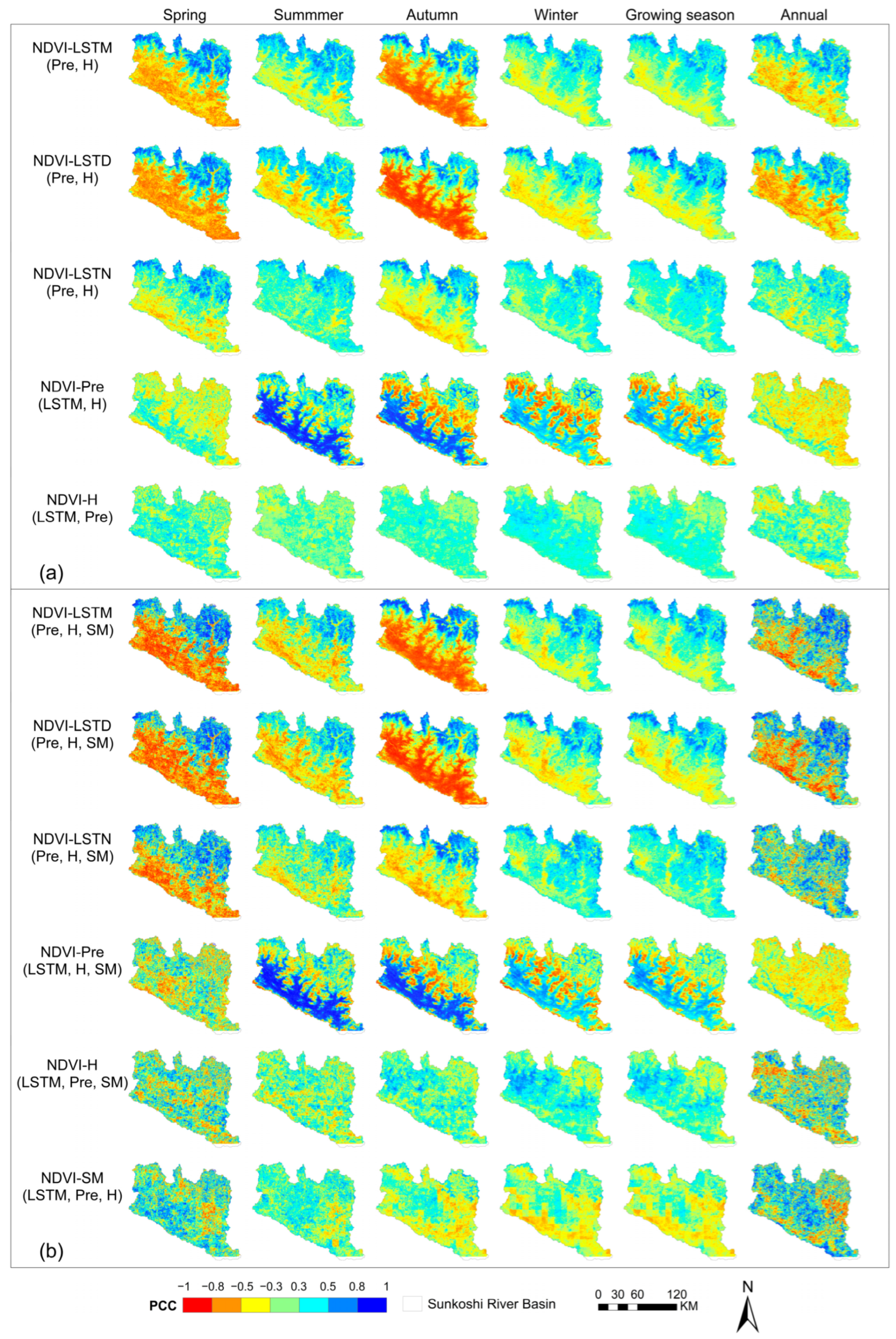
3.3.2. Spatial Heterogeneity of the Relationship Among NDVI and Climatic Factors and Soil Moisture

To explore the spatial difference of PCCs across the study area, Figure 5a illustrates the distribution of PCCs among climate factors and NDVI during 2000 and 2021, and Figure 5b presents the distribution of PCCs among NDVI, climate factors and soil moisture over the period of 2012 to 2021. It is evident that the dominant factors controlling NDVI changes vary along with time and space.
As indicated in Figure 5a, both LST and precipitation show high spatial heterogeneity of PCCs with NDVI, while PCCs between humidity and NDVI presents lower spatial disparity. High PCCs of LSTM-NDVI and LSTD-NDVI show that LSTD and LSTM primarily govern NDVI changes in the spring and autumn seasons. However, their negative PCCs are observed in low-altitude areas (below 3 km), while positive correlations are observed in high-altitude regions (above 3 km).
Moreover, Figure 5a indicates positive high PCCs between NDVI and precipitation along the river banks especially at summer and autumn scales. Humidity and NDVI exhibit a moderate positive correlation across various time scales.
On an annual scale, PCCs between NDVI and LSTM are stronger than that between NDVI and precipitation (Figure 5). However, due to the offsetting effect of the former’s negative and positive PCCs, the averaged PCC between NDVI and precipitation (−0.564, Table 4) was higher than that between NDVI and LSTM (−0.165, Table 4) over the whole watershed. The results imply that partial correlation analysis at the pixel scale can show more detailed spatial disparity information than that at the watershed scale.
Figure 5b presents distribution of PCCs among NDVI and climatic factors and soil moisture from 2012 to 2021. Overall, compared to scenarios (Figure 5a) where the influence of soil moisture is not excluded, the PCCs in Figure 5b become higher for both negative and positive values and show higher spatial disparity. It implies that the impacts of climate factors on NDVI are enhanced after excluding the influence of soil moisture. Specifically, in spring, NDVI change is dominated by LST with negative PCCs in areas with lower elevation and positive PCCs in areas with high elevation. In summer, winter and growing season, precipitation shows high positive PCCs, dominating NDVI change. In summer, all of LSTM, LSTD and precipitation indicate high impacts with high PCCs. PCCs between NDVI and precipitation exhibit higher spatial heterogeneity throughout the year except for spring and annual scale, while LST displays higher spatial heterogeneity throughout the year except for winter and growing season. Although during the winter and growing season, the PCCs between humidity and NDVI exhibit higher correlations in the western part of the watershed (with altitudes below 2 km), compared to LST and precipitation, the spatial heterogeneity of the PCCs between humidity and NDVI remains lower. Soil moisture exhibits a positive correlation with NDVI on an annual basis in most parts of the watershed.

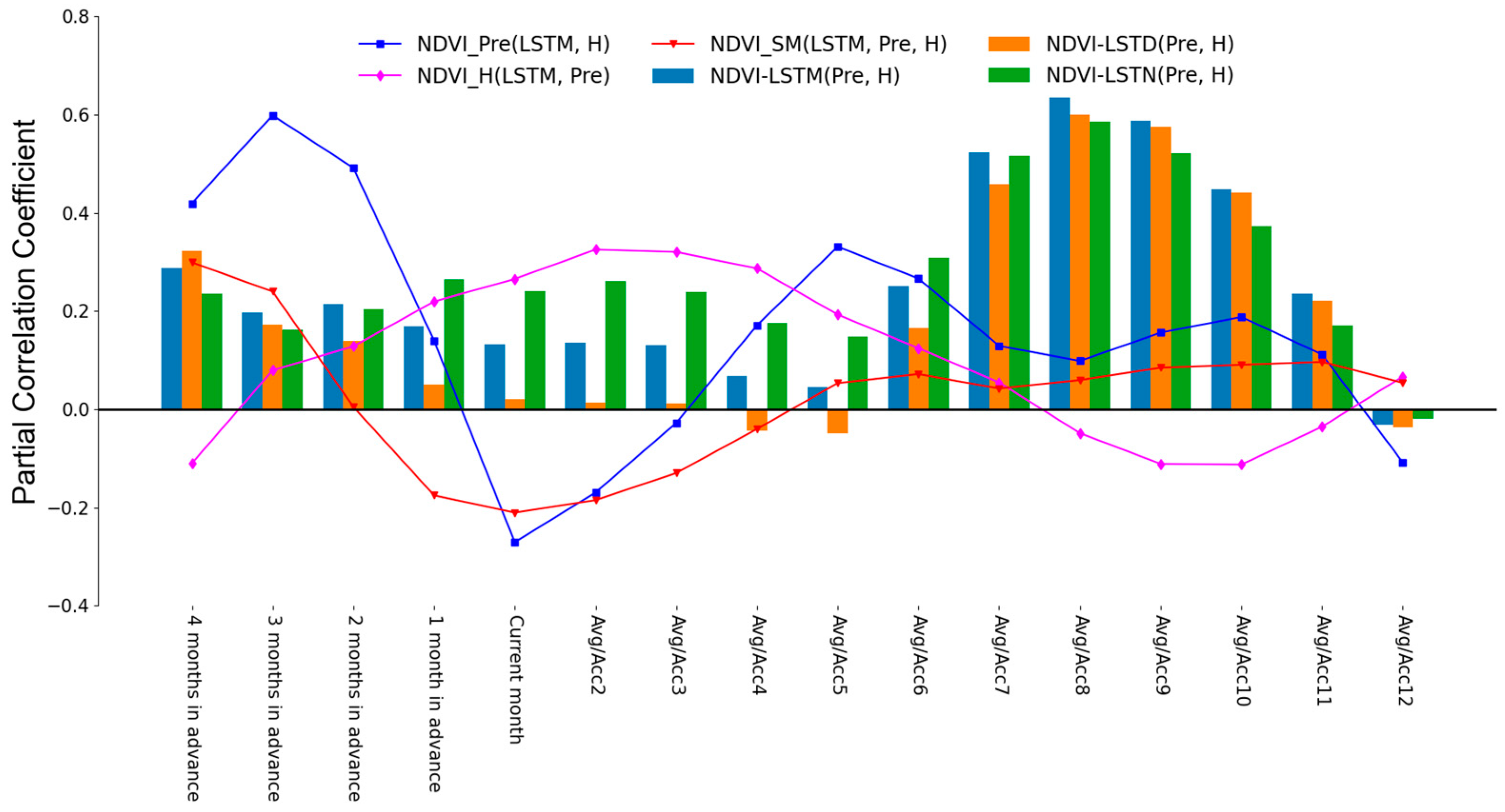
3.4. Lag and Cumulative Effects of Climate Factors and Soil Moisture on Vegetation

To investigate the lag and cumulative effects of climate factors and soil moisture on NDVI’s variation, four different lag periods (1–4 months) and eleven different accumulation periods (2–12 months) between impact factors and NDVI are set up. Subsequently, their PCCs are calculated and illustrated in Figure 6.
It can be observed that NDVI and precipitation with 3 months in advance achieved the highest PCC (0.60), which means that the lag effect of precipitation on NDVI change is 3 months. The PCC between NDVI and the accumulated precipitation arrived at the top (0.331) and then decreased with the accumulation period increasing from 2 to 8 months, which displays that the accumulation effect of precipitation on NDVI is 5 months. Humidity did not show any lag effect on NDVI, but showed an accumulation effect of 2 moths. And soil moisture exhibits a 4-month lag effect on change in NDVI. From Figure 6, it can also be observed that both the daytime LST and the mean LST show a lag effect of 4 months on NDVI change, while the nighttime LST only exhibits a 1-month lag effect. In contrast, PCCs between NDVI and LST reached the maximum values (LSTM: 0.635, LSTD: 0.600 and LSTN: 0.585) when the accumulated time was 8 months, indicating that LST has an obvious and consistent accumulation effect of 8 months on NDVI.

4. Discussion

4.1. Spatiotemporal Variation in the SKRW

The SKRB is a region sensitive to climate change, and its vegetation’s spatiotemporal variations have important implications for watershed management. Regarding temporal variation, annual NDVI increased significantly with a mean magnitude of 0.023/decade during 2000–2021, which is consistent with the study of Wu et al. [24]. As for intra-annual changes of NDVI, NDVI gradually increases from March to October, peaking in October, which aligns with the changes of climate factors and soil moisture (as shown in Figure 7). Climate factors and soil moisture from May to October exhibit favorable growth conditions for vegetation with abundant rainfall and suitable temperature (>12 °C), which may result in the increase in NDVI. However, the highest values of climate factors and soil moisture occurred in July instead of October, which is closely related to their lag and cumulative effects on vegetation. This phenomenon is also confirmed by the results in Section 3.4. In addition, this pattern may also be related to crops in the watershed. The crop planting calendar from Food and Agriculture Organization of the United Nations (http://www.fao.org/giews/countrybrief/country.jsp?code=NPL, accessed on 12 October 2024) documented that October is still the growing period for rice, and from December to February the next year is the growing season for wheat. As a rare example of successful community forestry, there has been an improvement in forest conditions nationwide in Nepal [53], especially in areas ranging from 1 km to 3 km. This also explains the observed large spatial and temporal heterogeneity, with a greening (improvement) trend dominating the entire watershed, particularly in the mid-elevation regions.

4.2. The Dominant Driving Factors of NDVI Change

Vegetation is primarily driven by hydrothermal conditions [54]. In the study area, the monsoon climate results in the synchrony of precipitation and temperature during the summer, with high temperatures and abundant rainfall typically corresponding to elevated vegetation indices. The repeated occurrence of this pattern over multiple years inevitably leads to a strong correlation between these two variables. Therefore, partial correlation analysis was employed in this study to more accurately reflect the true effects of hydrothermal conditions on vegetation.
The dominant driving factors of NDVI change in the Sunkoshi River watershed exhibit significant variation across different time and spatial scales. At the annual scale, precipitation and daytime LST are the main controlling factors, which is consistent with previous studies [23,24]. During spring, summer, and winter, temperature is the primary factor influencing vegetation growth. In spring, rising daytime LST is associated with a decrease in NDVI [55], whereas in summer, NDVI shows a significant positive correlation with LST, which is mainly because higher temperature during this season enhances photosynthesis and promotes vegetation growth [56]. In winter, excessively high temperatures can intensify respiration, which is detrimental to vegetation growth [57]. Furthermore, the relationship between NDVI and daytime LST displays a clear elevation dependence; NDVI and LST are negatively correlated in low-altitude areas and exhibit positive correlation in high-altitude regions. This is because in low-altitude areas, rising LST will intensify vegetation respiration, which is not conducive to vegetation growth. Additionally, vegetation possesses cooling capabilities [58]. Conversely, in high-altitude regions, vegetation growth is limited by LST [59] and rising LST can promote vegetation growth [60].
Precipitation is the direct source of water supply, and its amount directly influences vegetation productivity and coverage, especially during the growing season [61]. Due to the influence of the monsoon climate, precipitation becomes the primary factor influencing vegetation both annually and throughout the growing season. The spatial distribution of PCCs between NDVI and precipitation indicates that precipitation exhibits a strong positive correlation with NDVI in low- and mid-elevation areas during summer, autumn, winter, and the growing season. However, in high altitude regions, where temperature is low and snowmelt contributes significantly to water availability, precipitation is not the primary factor influencing vegetation growth [62].
Soil moisture content exhibits a positive correlation with NDVI on an annual basis across the entire watershed. This positive association is attributed to the fact that elevated levels of soil moisture facilitate the uptake of water by plants [63]. When the influence of soil moisture is excluded, the PCCs between precipitation, LST, and NDVI increase significantly, indicating that soil moisture plays a key mediating role between climate and vegetation. High humidity inhibits the rate of transpiration in plants, which is conducive to the accumulation of organic matter [64]. Consequently, humidity exhibits a moderate positive correlation with NDVI.

4.3. Lag and Cumulative Effects of Impact Factors on NDVI Response

In this study, the lag and cumulative effects of climatic factors on NDVI were also considered, which would enhance the understanding of vegetation feedback dynamics. The results indicate that climatic factors and soil moisture exhibit significant lag or cumulative effects on vegetation change. One explanation for the observed lag and cumulative effects is that the influencing factors impact physiological processes and other non-climatic conditions. The lag effect of precipitation on vegetation reflects the time taken for water to reach plant roots after rainfall occurs [65]. At the individual plant scale, appropriate soil moisture, temperature, or precipitation levels are required to initiate the plant life cycle (i.e., seed germination, seedling growth, flowering), manifesting as lag or cumulative effects [43,66,67]. At the ecosystem scale, biogeochemical cycles that provide soil nutrients for plant absorption and growth also require cumulative time effects, such as the accumulation of temperature [68,69].

4.4. The Limitation of This Study

Resampling is a key step of data preprocessing. In this study, the widely used nearest neighbor interpolation method is adopted to resample different raster datasets into the same resolution. This method is computationally efficient, widely used in remote sensing and vegetation studies, and helps to preserve the original measured or classified values, especially for categorical or highly variable datasets. However, the disadvantage of this method is the lack of continuity and smooth transition when the image is enlarged. Therefore, more advanced downscaling techniques (such as bicubic interpolation, Spline interpolation) are suggested, especially for areas having sufficient in situ observation data supported.
Due to the data limitation, this work only studies the response of NDVI to some limited key climate factors (land surface temperature, precipitation, humidity) and soil moisture. In fact, vegetation is affected by many other factors including atmospheric pressure, duration of sunlight, evaporation, soil properties, land use, etc. Therefore, more variables and longer terms can be investigated and more comprehensive studies can be conducted in the future, especially when more related datasets become available. Furthermore, vegetation change can be quantitatively attributed to climate change and human activities.

5. Conclusions

This study assessed the spatiotemporal variations in NDVI in the Sunkoshi River watershed during 2000–2021 and identified the driving factors behind vegetation change at different scales. Key conclusions are as follows. (1) NDVI shows seasonality, increasing since March and reaching the peak in October. (2) Annual NDVI in 90.9% of the study area increased with a mean magnitude of 0.023/decade during 2000–2021, but the trends exhibit spatial heterogeneity. (3) The dominant driving factors of NDVI change vary along with different factors considered, and different time scales. Daytime LST dominates NDVI changes in spring, summer and winter during 2000–2021. Excluding the interference of soil moisture enhances the impacts of LST and precipitation on NDVI, reflected by higher PCCs between climate factors and NDVI and stronger spatial heterogeneity. (4) Precipitation shows a 3-month lag effect and a 5-month cumulative effect on NDVI; the LST has an 8-month cumulative effect and the daytime LST and the nighttime LST have a 4-month and 11-month lag effect on NDVI, respectively; humidity exhibits a 2-month cumulative effect on NDVI and exhibits no lag effect; soil moisture indicates a 4-month lag effect on NDVI and shows no cumulative effect. The findings in this study deepen our understanding of vegetation–climate–soil moisture interactions in the Himalayas, highlight the significance of multi-scale and multi-factor analyses, and provide a scientific foundation for ecological conservation and climate adaptation planning in Nepal. To address the limitations of this study, future research should incorporate additional influencing factors (such as atmospheric pressure, duration of sunlight, and topographic variables) and quantitatively distinguish the contributions of climate change and human activities to vegetation dynamics.

Author Contributions

Z.J.: formal analysis, visualization, writing original draft; Q.Y.: funding acquisition; methodology, supervision, writing original draft, review and editing; J.S.: supervision, funding acquisition, review and editing; G.W.: funding acquisition, review and editing; V.P.P.: data support, review and editing. All authors have read and agreed to the published version of the manuscript.

Funding

This work has been financially supported by the [National Key Research and Development Program of China] under Grant [number 2021YFC3201100]; [National Natural Science Foundation of China] under Grant [number 62376054]; [Sichuan Province Science and Technology Support Program] under Grant [numbers 2024NSFSC0063; 2025YFHZ0236; DQ202411]; [Open Foundation of Key Laboratory of Taihu Basin Water Re-sources Management, Ministry of Water Resources] under Grant [number Yk924004-C8]; [Aeronautical Science Foundation] under Grant [number 2024M071080003]; [Municipal Government of Quzhou] under Grant [number 2023D016]; [Guangdong Basic and Applied Basic Research Foundation] under Grant [number 2024A1515011634]; and [Shenzhen Science and Technology Program] under Grant [number JCYJ20230807120008016].

Data Availability Statement

All the data are available from the web links provided in Table 1 in the text.

Conflicts of Interest

The authors declare no conflicts of interest.

References

  1. Zhu, Z.; Fu, Y.; Woodcock, C.E.; Olofsson, P.; Vogelmann, J.E.; Holden, C.; Wang, M.; Dai, S.; Yu, Y. Including land cover change in analysis of greenness trends using all available Landsat 5, 7, and 8 images: A case study from Guangzhou, China (2000–2014). Remote Sens. Environ. 2016, 185, 243–257. [Google Scholar] [CrossRef]
  2. Wu, C.; Venevsky, S.; Sitch, S.; Yang, Y.; Wang, M.; Wang, L.; Gao, Y. Present-day and future contribution of climate and fires to vegetation composition in the boreal forest of China. Ecosphere 2017, 8, e01917. [Google Scholar] [CrossRef]
  3. Przeździecki, K.M.; Zawadzki, J.; Cieszewski, C.; Bettinger, P. Estimation of soil moisture across broad landscapes of Georgia and South Carolina using the triangle method applied to MODIS satellite imagery. Silva Fenn. 2017, 51, 1683. [Google Scholar] [CrossRef]
  4. Bo-Tao, Z.; Jin, Q. Changes of weather and climate extremes in the IPCC AR6. Adv. Clim. Change Res. 2021, 17, 713. [Google Scholar]
  5. Yang, Q.; Zhang, H.; Peng, W.; Lan, Y.; Luo, S.; Shao, J.; Chen, D.; Wang, G. Assessing climate impact on forest cover in areas undergoing substantial land cover change using Landsat imagery. Sci. Total Environ. 2019, 659, 732–745. [Google Scholar] [CrossRef]
  6. He, L.; Guo, J.; Yang, W.; Jiang, Q.; Chen, L.; Tang, K. Multifaceted responses of vegetation to average and extreme climate change over global drylands. Sci. Total Environ. 2023, 858, 159942. [Google Scholar] [CrossRef]
  7. Li, P.; Wang, J.; Liu, M.; Xue, Z.; Bagherzadeh, A.; Liu, M. Spatio-temporal variation characteristics of NDVI and its response to climate on the Loess Plateau from 1985 to 2015. Catena 2021, 203, 105331. [Google Scholar] [CrossRef]
  8. Vrac, M.; Thao, S.; Yiou, P. Changes in temperature–precipitation correlations over Europe: Are climate models reliable? Clim. Dyn. 2023, 60, 2713–2733. [Google Scholar] [CrossRef]
  9. Li, W.; Chen, R.; Ma, D.; Wang, C.; Yang, Y.; Wang, C.; Chen, H.; Yin, G. Tracking autumn photosynthetic phenology on Tibetan plateau grassland with the green–red vegetation index. Agric. For. Meteorol. 2023, 339, 109573. [Google Scholar] [CrossRef]
  10. Stisen, S.; Sandholt, I.; Nørgaard, A.; Fensholt, R.; Eklundh, L. Estimation of diurnal air temperature using MSG SEVIRI data in West Africa. Remote Sens. Environ. 2007, 110, 262–274. [Google Scholar] [CrossRef]
  11. Liu, Y.; Li, Y.; Li, S.; Motesharrei, S. Spatial and temporal patterns of global NDVI trends: Correlations with climate and human factors. Remote Sens. 2015, 7, 13233–13250. [Google Scholar] [CrossRef]
  12. Chen, B.-M.; Gao, Y.; Liao, H.-X.; Peng, S.-L. Differential responses of invasive and native plants to warming with simulated changes in diurnal temperature ranges. AoB Plants 2017, 9, plx028. [Google Scholar] [CrossRef]
  13. Wu, H.; Xiong, D.; Liu, B.; Zhang, S.; Yuan, Y.; Fang, Y.; Chidi, C.L.; Dahal, N.M. Spatio-temporal analysis of drought variability using CWSI in the Koshi River Basin (KRB). Int. J. Environ. Res. Public Health 2019, 16, 3100. [Google Scholar] [CrossRef]
  14. Peng, S.S.; Chen, A.P.; Xu, L.; Cao, C.X.; Fang, J.Y.; Myneni, R.B.; Pinzon, J.E.; Tucker, C.J.; Piao, S.L. Recent change of vegetation growth trend in China. Environ. Res. Lett. 2011, 6, 044027. [Google Scholar] [CrossRef]
  15. Sun, H.; Wang, J.; Xiong, J.; Bian, J.; Jin, H.; Cheng, W.; Li, A.; Mozo, H.G. Vegetation change and its response to climate change in Yunnan Province, China. Adv. Meteorol. 2021, 2021, 8857589. [Google Scholar] [CrossRef]
  16. Liu, H.; Tian, F.; Hu, H.; Hu, H.; Sivapalan, M. Soil moisture controls on patterns of grass green-up in Inner Mongolia: An index based approach. Hydrol. Earth Syst. Sci. 2013, 17, 805–815. [Google Scholar] [CrossRef]
  17. Mohanty, B.P.; Skaggs, T. Spatio-temporal evolution and time-stable characteristics of soil moisture within remote sensing footprints with varying soil, slope, and vegetation. Adv. Water Resour. 2001, 24, 1051–1067. [Google Scholar] [CrossRef]
  18. Yang, L.; Wei, W.; Chen, L.; Chen, W.; Wang, J. Response of temporal variation of soil moisture to vegetation restoration in semi-arid Loess Plateau, China. Catena 2014, 115, 123–133. [Google Scholar] [CrossRef]
  19. Vreugdenhil, M.; Dorigo, W.A.; Wagner, W.; De Jeu, R.A.; Hahn, S.; Van Marle, M.J. Analyzing the vegetation parameterization in the TU-Wien ASCAT soil moisture retrieval. IEEE Trans. Geosci. Remote Sens. 2016, 54, 3513–3531. [Google Scholar] [CrossRef]
  20. Nandintsetseg, B.; Shinoda, M.; Kimura, R.; Ibaraki, Y. Relationship between soil moisture and vegetation activity in the Mongolian steppe. Sola 2010, 6, 29–32. [Google Scholar] [CrossRef]
  21. Li, W.; Migliavacca, M.; Forkel, M.; Denissen, J.M.C.; Reichstein, M.; Yang, H.; Duveiller, G.; Weber, U.; Orth, R. Widespread increasing vegetation sensitivity to soil moisture. Nat. Commun. 2022, 13, 3959. [Google Scholar] [CrossRef]
  22. Bajracharya, S.R.; Pradhananga, S.; Shrestha, A.B.; Thapa, R. Future climate and its potential impact on the spatial and temporal hydrological regime in the Koshi Basin, Nepal. J. Hydrol. Reg. Stud. 2023, 45, 101316. [Google Scholar] [CrossRef]
  23. Zhang, Y.; Gao, J.; Liu, L.; Wang, Z.; Ding, M.; Yang, X. NDVI-based vegetation changes and their responses to climate change from 1982 to 2011: A case study in the Koshi River Basin in the middle Himalayas. Glob. Planet. Change 2013, 108, 139–148. [Google Scholar] [CrossRef]
  24. Wu, X.; Sun, X.; Wang, Z.; Zhang, Y.; Liu, Q.; Zhang, B.; Paudel, B.; Xie, F. Vegetation changes and their response to global change based on NDVI in the Koshi river Basin of central Himalayas since 2000. Sustainability 2020, 12, 6644. [Google Scholar] [CrossRef]
  25. Banjara, P.; Pandey, V.P.; Shrestha, P.K. Drought Risk Assessment in Sunkoshi River Basin: An Application of Hydrological Model. In Proceedings of the 12th IOE Graduate Conference, Kathmandu, Nepal, 19–22 October 2022. [Google Scholar]
  26. Ehrlich, D.; Estes, J.E.; Singh, A. Applications of NOAA-AVHRR 1 km data for environmental monitoring. Remote Sens. 1994, 15, 145–161. [Google Scholar] [CrossRef]
  27. Ma, Y.; He, T.; McVicar, T.R.; Liang, S.; Liu, T.; Peng, W.; Song, D.-X.; Tian, F. Quantifying how topography impacts vegetation indices at various spatial and temporal scales. Remote Sens. Environ. 2024, 312, 114311. [Google Scholar] [CrossRef]
  28. Coll, C.; Caselles, V.; Galve, J.; Valor, E.; Niclos, R.; Sanchez, J.; Rivas, R. Ground measurements for the validation of land surface temperatures derived from AATSR and MODIS data. Remote Sens. Environ. 2005, 97, 288–300. [Google Scholar] [CrossRef]
  29. Peng, G.; Li, J.; Chen, Y.; Norizan, A.P.; Tay, L. High-resolution surface relative humidity computation using MODIS image in Peninsular Malaysia. Chin. Geogr. Sci. 2006, 16, 260–264. [Google Scholar] [CrossRef]
  30. Famiglietti, C.A.; Fisher, J.B.; Halverson, G.; Borbas, E.E. Global validation of MODIS near-surface air and dew point temperatures. Geophys. Res. Lett. 2018, 45, 7772–7780. [Google Scholar] [CrossRef]
  31. Huffman, G.J.; Bolvin, D.T.; Braithwaite, D.; Hsu, K.; Joyce, R.; Xie, P.; Yoo, S.H. NASA Global Precipitation Measurement (GPM) Integrated Multi-Satellite Retrievals for GPM (IMERG); Algorithm theoretical basis document (ATBD) version; National Aeronautics and Space Administration: Washington, DC, USA, 2015; Volume 4, p. 30.
  32. Xu, F.; Guo, B.; Ye, B.; Ye, Q.; Chen, H.; Ju, X.; Guo, J.; Wang, Z. Systematical evaluation of GPM IMERG and TRMM 3B42V7 precipitation products in the Huang-Huai-Hai Plain, China. Remote Sens. 2019, 11, 697. [Google Scholar] [CrossRef]
  33. Xu, R.; Tian, F.; Yang, L.; Hu, H.; Lu, H.; Hou, A. Ground validation of GPM IMERG and TRMM 3B42V7 rainfall products over southern Tibetan Plateau based on a high-density rain gauge network. J. Geophys. Res. Atmos. 2017, 122, 910–924. [Google Scholar] [CrossRef]
  34. Kim, K.; Park, J.; Baik, J.; Choi, M. Evaluation of topographical and seasonal feature using GPM IMERG and TRMM 3B42 over Far-East Asia. Atmos. Res. 2017, 187, 95–105. [Google Scholar] [CrossRef]
  35. Liu, J.; Huang, B.; Chen, L.; Yang, J.; Chen, X. Evaluation of GPM and TRMM and their capabilities for capturing solid and light precipitations in the headwater basin of the Heihe River. Atmosphere 2023, 14, 453. [Google Scholar] [CrossRef]
  36. Kim, S.; Liu, Y.Y.; Johnson, F.M.; Parinussa, R.M.; Sharma, A. A global comparison of alternate AMSR2 soil moisture products: Why do they differ? Remote Sens. Environ. 2015, 161, 43–62. [Google Scholar] [CrossRef]
  37. Li, J.; Heap, A.D. A Review of Spatial Interpolation Methods for Environmental Scientists; Geoscience Australia: Canberra, ACT, Australia, 2008.
  38. Brandsma, T.; Können, G.P. Application of nearest-neighbor resampling for homogenizing temperature records on a daily to sub-daily level. Int. J. Climatol. 2006, 26, 75–89. [Google Scholar] [CrossRef]
  39. Zhu, Z.; Woodcock, C.E. Object-based cloud and cloud shadow detection in Landsat imagery. Remote Sens. Environ. 2012, 118, 83–94. [Google Scholar] [CrossRef]
  40. Jiang, W.; Yuan, L.; Wang, W.; Cao, R.; Zhang, Y.; Shen, W. Spatio-temporal analysis of vegetation variation in the Yellow River Basin. Ecol. Indic. 2015, 51, 117–126. [Google Scholar] [CrossRef]
  41. Chu, H.; Venevsky, S.; Wu, C.; Wang, M. NDVI-based vegetation dynamics and its response to climate changes at Amur-Heilongjiang River Basin from 1982 to 2015. Sci. Total Environ. 2019, 650, 2051–2062. [Google Scholar] [CrossRef]
  42. Rajbhandari, R.; Shrestha, A.B.; Nepal, S.; Wahid, S. Projection of future climate over the Koshi River basin based on CMIP5 GCMs. Atmos. Clim. Sci. 2016, 6, 190–204. [Google Scholar] [CrossRef]
  43. Aguilar, C.; Zinnert, J.C.; Polo, M.J.; Young, D.R. NDVI as an indicator for changes in water availability to woody vegetation. Ecol. Indic. 2012, 23, 290–300. [Google Scholar] [CrossRef]
  44. Zhu, Z.; Piao, S.; Myneni, R.B.; Huang, M.; Zeng, Z.; Canadell, J.G.; Ciais, P.; Sitch, S.; Friedlingstein, P.; Arneth, A.; et al. Greening of the Earth and its drivers. Nat. Clim. Change 2016, 6, 791–795. [Google Scholar] [CrossRef]
  45. Di Leo, G.; Sardanelli, F. Statistical significance: P value, 0.05 threshold, and applications to radiomics—Reasons for a conservative approach. Eur. Radiol. Exp. 2020, 4, 18. [Google Scholar] [CrossRef]
  46. Lou, J.; Xu, G.; Wang, Z.; Yang, Z.; Ni, S. Multi-year NDVI values as indicator of the relationship between spatiotemporal vegetation dynamics and environmental factors in the Qaidam Basin, China. Remote Sens. 2021, 13, 1240. [Google Scholar] [CrossRef]
  47. Andrade, C. The P value and statistical significance: Misunderstandings, explanations, challenges, and alternatives. Indian J. Psychol. Med. 2019, 41, 210–215. [Google Scholar] [CrossRef]
  48. Cleveland, R.B.; Cleveland, W.S.; McRae, J.E.; Terpenning, I. STL: A seasonal-trend decomposition. J. Off. Stat. 1990, 6, 3–73. [Google Scholar]
  49. Mann, H.B. Nonparametric tests against trend. Econometrica 1945, 13, 245–259. [Google Scholar] [CrossRef]
  50. Wang, F.; Shao, W.; Yu, H.; Kan, G.; He, X.; Zhang, D.; Ren, M.; Wang, G. Re-evaluation of the power of the Mann-Kendall test for detecting monotonic trends in hydrometeorological time series. Front. Earth Sci. 2020, 8, 14. [Google Scholar] [CrossRef]
  51. Kenett, D.Y.; Huang, X.; Vodenska, I.; Havlin, S.; Stanley, H.E. Partial correlation analysis: Applications for financial markets. Quant. Financ. 2015, 15, 569–578. [Google Scholar] [CrossRef]
  52. Van Aert, R.C.; Goos, C. A critical reflection on computing the sampling variance of the partial correlation coefficient. Res. Synth. Methods 2023, 14, 520–525. [Google Scholar] [CrossRef]
  53. Gautam, A.P.; Shivakoti, G.P.; Webb, E.L. A review of forest policies, institutions, and changes in the resource condition in Nepal. Int. For. Rev. 2004, 6, 136–148. [Google Scholar] [CrossRef]
  54. Wang, S.; Li, R.; Wu, Y.; Zhao, S. Vegetation dynamics and their response to hydrothermal conditions in Inner Mongolia, China. Glob. Ecol. Conserv. 2022, 34, e02034. [Google Scholar] [CrossRef]
  55. Chuai, X.W.; Huang, X.J.; Wang, W.J.; Bao, G. NDVI, temperature and precipitation changes and their relationships with different vegetation types during 1998–2007 in Inner Mongolia, China. Int. J. Climatol. 2013, 33, 1696–1706. [Google Scholar] [CrossRef]
  56. Crous, K.Y.; Uddling, J.; De Kauwe, M.G. Temperature responses of photosynthesis and respiration in evergreen trees from boreal to tropical latitudes. New Phytol. 2022, 234, 353–374. [Google Scholar] [CrossRef]
  57. Niu, S.; Chen, W.; Liáng, L.L.; Sierra, C.A.; Xia, J.; Wang, S.; Heskel, M.; Patel, K.F.; Bond-Lamberty, B.; Wang, J.; et al. Temperature responses of ecosystem respiration. Nat. Rev. Earth Environ. 2024, 5, 559–571. [Google Scholar] [CrossRef]
  58. Zhou, S.; Zheng, H.; Liu, X.; Gao, Q.; Xie, J. Identifying the effects of vegetation on urban surface temperatures based on urban–rural local climate zones in a subtropical metropolis. Remote Sens. 2023, 15, 4743. [Google Scholar] [CrossRef]
  59. Schultz, P.; Halpert, M. Global correlation of temperature, NDVI and precipitation. Adv. Space Res. 1993, 13, 277–280. [Google Scholar] [CrossRef]
  60. Dusenge, M.E.; Duarte, A.G.; Way, D.A. Plant carbon metabolism and climate change: Elevated CO2 and temperature impacts on photosynthesis, photorespiration and respiration. New Phytol. 2019, 221, 32–49. [Google Scholar] [CrossRef]
  61. Zeppel, M.J.B.; Wilks, J.V.; Lewis, J.D. Impacts of extreme precipitation and seasonal changes in precipitation on plants. Biogeosciences 2014, 11, 3083–3093. [Google Scholar] [CrossRef]
  62. Chen, X.; Guan, T.; Zhang, J.; Liu, Y.; Jin, J.; Liu, C.; Wang, G.; Bao, Z. Identifying and predicting the responses of multi-altitude vegetation to climate change in the Alpine zone. Forests 2024, 15, 308. [Google Scholar] [CrossRef]
  63. Xie, B.; Qin, Z.; Wang, Y.; Chang, Q. Monitoring vegetation phenology and their response to climate change on Chinese Loess Plateau based on remote sensing. Trans. Chin. Soc. Agric. Eng. 2015, 31, 153–160. [Google Scholar]
  64. Grantz, D.A. Plant response to atmospheric humidity. Plant Cell Environ. 1990, 13, 667–679. [Google Scholar] [CrossRef]
  65. Jobbágy, E.G.; Sala, O.E.; Paruelo, J.M. Patterns and controls of primary production in the Patagonian steppe: A remote sensing approach. Ecology 2002, 83, 307–319. [Google Scholar]
  66. Busetto, L.; Colombo, R.; Migliavacca, M.; Cremonese, E.; Meroni, M.; Galvagno, M.; Rossini, M.; Siniscalco, C.; DICella, U.M.; Pari, E. Remote sensing of larch phenological cycle and analysis of relationships with climate in the Alpine region. Glob. Change Biol. 2010, 16, 2504–2517. [Google Scholar] [CrossRef]
  67. Zhang, H.; Liu, S.; Regnier, P.; Yuan, W. New insights on plant phenological response to temperature revealed from long-term widespread observations in China. Glob. Change Biol. 2018, 24, 2066–2078. [Google Scholar] [CrossRef]
  68. Braswell, B.; Schimel, D.S.; Linder, E.; Moore Iii, B. The response of global terrestrial ecosystems to interannual temperature variability. Science 1997, 278, 870–873. [Google Scholar] [CrossRef]
  69. Ivits, E.; Horion, S.; Erhard, M.; Fensholt, R. Assessing European ecosystem stability to drought in the vegetation growing season. Glob. Ecol. Biogeogr. 2016, 25, 1131–1143. [Google Scholar] [CrossRef]
Figure 1. Location and elevation of the study area (the Sunkoshi River watershed).
Water 17 02232 g001
Figure 2. Inter-annual (a) and intra-annual (b) change of NDVI in the Sunkoshi River watershed during 2000–2021.
Water 17 02232 g002
Figure 3. The results of STL decomposition of NDVI during 2001–2021 and the result of MK test on trend component of NDVI (the red dashed line).
Water 17 02232 g003
Figure 4. Distribution of change rate of NDVI in the SKRW based on the simple linear trend (SLT) method over the period 2000–2021 (af) and distribution of NDVI trend types with statistical significance (gl). (af) and (gl) correspond to spring, summer, autumn, winter, growing season and annual scale, respectively.
Water 17 02232 g004
Figure 5. The distribution of PCCs between NDVI and impact factors at different time scales. (a) The distribution of PCCs between NDVI and climate factors at seasonal and annual scales during 2000–2021; (b) the distribution of PCCs among NDVI and climate factors and soil moisture at seasonal and annual scales during 2012–2021.
Water 17 02232 g005
Figure 6. Lag and accumulation effects of climatic factors and soil moisture on NDVI. Avg/Acc i (i = 2, 3, 4, …, 12) represents the average temperature or the accumulative precipitation of i months.
Water 17 02232 g006
Figure 7. The intra-annual changes of land surface temperature (a), precipitation (b), humidity (c) and soil moisture (d) in the Sunkoshi River watershed.
Water 17 02232 g007
Table 1. The basic information of data used in this study.
VariableName of DatasetTime PeriodTemporal ResolutionSpatial ResolutionAccess Link
NDVIMOD13A12000–202116 days500 mhttps://search.earthdata.nasa.gov/search/granules?p=C194001237-LPDAAC_ECS&pg[0][v]=f&pg[0][gsk]=-start_date&q=MOD13A1&tl=1658478390.768!3!! (accessed on 20 June 2024).
LSTMOD11A22000–20218 days1 kmhttps://search.earthdata.nasa.gov/search/granules?p=C194001212-LPDAAC_ECS&pg[0][v]=f&pg[0][gsk]=-start_date&q=MOD11A2&tl=1658478390!3!! (accessed on 20 June 2024).
PrecipitationGPM IMERG2000–2021daily0.1°https://search.earthdata.nasa.gov/search/granules?p=C1598621092-GES_DISC&pg[0][v]=f&pg[0][gsk]=-start_date&q=GPM%20IMERG%20Final%20Precipitation&tl=1658478390!3!! (accessed on 20 June 2024).
HumidityMOD072000–2021daily5 kmhttps://search.earthdata.nasa.gov/search/granules?p=C1443541366-LAADS&pg[0][v]=f&pg[0][gsk]=-start_date&q=MODIS/Terra%20syysTemperature%20and%20Water%20Vapor%20Profiles%205-Min%20L2%20Swath%205km&tl=1716917951.185!3!! (accessed on 20 June 2024).
Soil moistureAMSR22012–2021monthly10 kmhttps://search.earthdata.nasa.gov/search/granules?p=C1235316218-GES_DISC&pg[0][v]=f&pg[0][gsk]=-start_date&q=%20AMSR2/GCOM-W1&tl=1658478390!3!! (accessed on 20 June 2024).
ElevationDEM//30 mhttp://www.gscloud.cn/
Note: NDVI, Normalized Difference Vegetation Index; LST, land surface temperature.
Table 2. Statistics of NDVI change during 2000–2021 in the Sunkoshi River watershed based on the simple linear trend (SLT) model.
SpringSummerAutumnWinterGrowing SeasonAnnual
Change rate (/year)0.0027 **0.01140.0023 **0.0024 **0.0021 *0.0023 **
Note: NDVI, Normalized Difference Vegetation Index; * and ** represent significance levels of 0.05 and 0.01, respectively.
Table 3. Statistical result of the NDVI trend types based on Figure 4.
ImprovementDegradation
High Sig.Weak Sig.Non-Sig.SumHigh Sig.Weak Sig.Non-Sig.Sum
Spring33.6%12.5%40.3%86.4%0.2%0.1%13.3%13.6%
Summer8.3%9.8%62.4%80.5%0.4%0.1%19.0%19.5%
Autumn45.513.6%32.9%92.0%0.3%0.1%7.6%8.0%
Winter45.610.6%30.0%86.2%1.1%0.8%11.9%13.8%
Growing Season13.813.2%58.6%85.6%0.3%0.1%15.5%15.9%
Annual38.614%38.3%90.9%0.5%0.4%8.2%9.1%
Note: Sig., significance.
Table 4. Partial correlation coefficients between NDVI and climate factors at different time scales during 2000–2021 in the Sunkoshi River watershed.
NDVI-LSTM
(Pre, H)
NDVI-LSTD
(Pre, H)
NDVI-LSTN
(Pre, H)
NDVI-Pre
(LSTM, H)
NDVI-Pre
(LSTD, H)
NDVI-Pre
(LSTN, H)
NDVI-H
(LSTM, Pre)
Spring−0.299−0.4820.111−0.125−0.1150.0310.344
Summer0.5890.6580.372−0.085−0.134−0.149−0.361
Autumn0.048−0.0670.188−0.165−0.2−0.0970.322
Winter−0.361−0.525−0.129−0.432−0.432−0.2720.089
Growing Season0.2880.2170.255−0.389−0.416−0.382−0.210
Monthly0.1330.020.241−0.271−0.304−0.382−0.210
Seasonal0.093−0.0470.299−0.056−0.059−0.193−0.208
Annual−0.165−0.3690.152−0.564−0.550−0.4630.092
Note: NDVI, normalized vegetation index; LSTM, the mean value of daytime LST and nighttime LST; LSTD, daytime LST; LSTN, nighttime LST; Pre, precipitation; H, humidity. A-B (C, D) indicates the partial correlation coefficient between A and B after excluding the influences of C and D. The number in bold indicates that its corresponding impact factor dominates NDVI change on the corresponding time scale.
Table 5. Partial correlation coefficients among NDVI, climate factors and soil moisture at different time scales during 2012–2021 in the Sunkoshi River watershed.
NDVI-LSTM
(Pre, H, SM)
NDVI-LSTD
(Pre, H, SM)
NDVI-LSTN
(Pre, H, SM)
NDVI-Pre
(LSTM, H, SM)
NDVI-H
(LSTM, Pre, SM)
NDVI-SM
(LSTM, Pre, H)
Spring−0.212−0.3570.1640.009−0.0090.234
Summer−0.096−0.167−0.0580.1000.0850.322
Autumn−0.655−0.716−0.315−0.4730.6970.261
Winter−0.176−0.3140.036−0.310.571−0.055
Growing Season−0.122−0.2490.072−0.2230.523−0.131
Monthly0.2160.0910.3680.204−0.330−0.417
Seasonal0.2560.1540.327−0.0580.199−0.211
Annual0.4870.3190.610−0.785−0.0570.681
Note: SM, soil moisture. A–B (C, D, E) indicate the partial correlation coefficient between A and B after excluding the influences of C, D and E. The number in bold indicates that its corresponding impact factor dominates NDVI change on the corresponding time scale.
Disclaimer/Publisher’s Note: The statements, opinions and data contained in all publications are solely those of the individual author(s) and contributor(s) and not of MDPI and/or the editor(s). MDPI and/or the editor(s) disclaim responsibility for any injury to people or property resulting from any ideas, methods, instructions or products referred to in the content.

