
A Climatology of Errors in HREF MCS Precipitation Objects


Abstract
1. Introduction
2. Data and Methods
2.1. Data
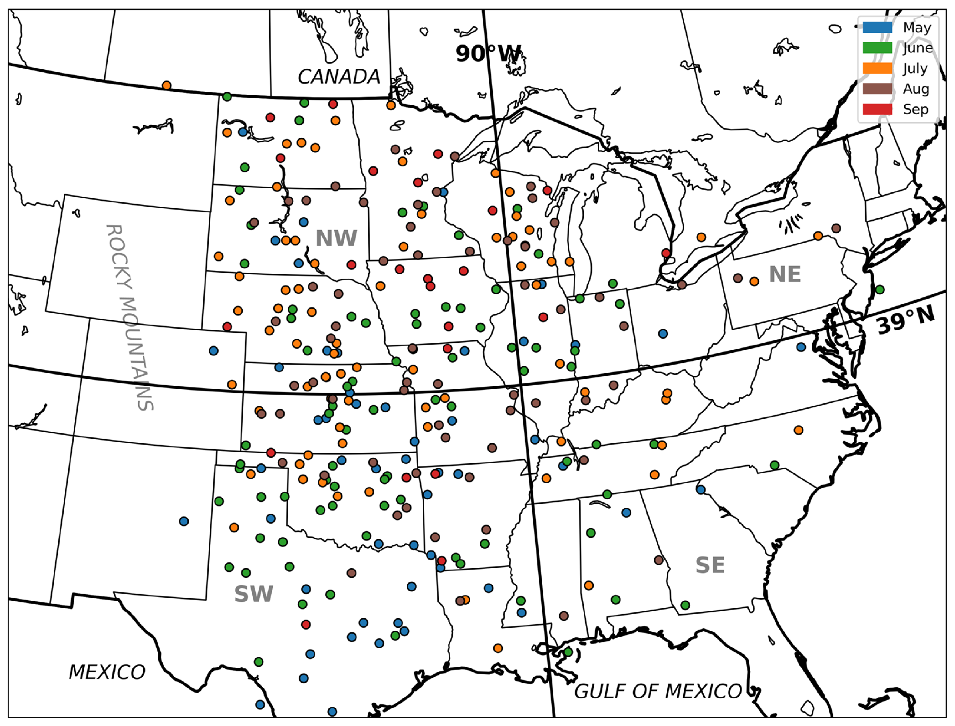
2.2. Case Selection
2.3. MODE Processing
3. Results
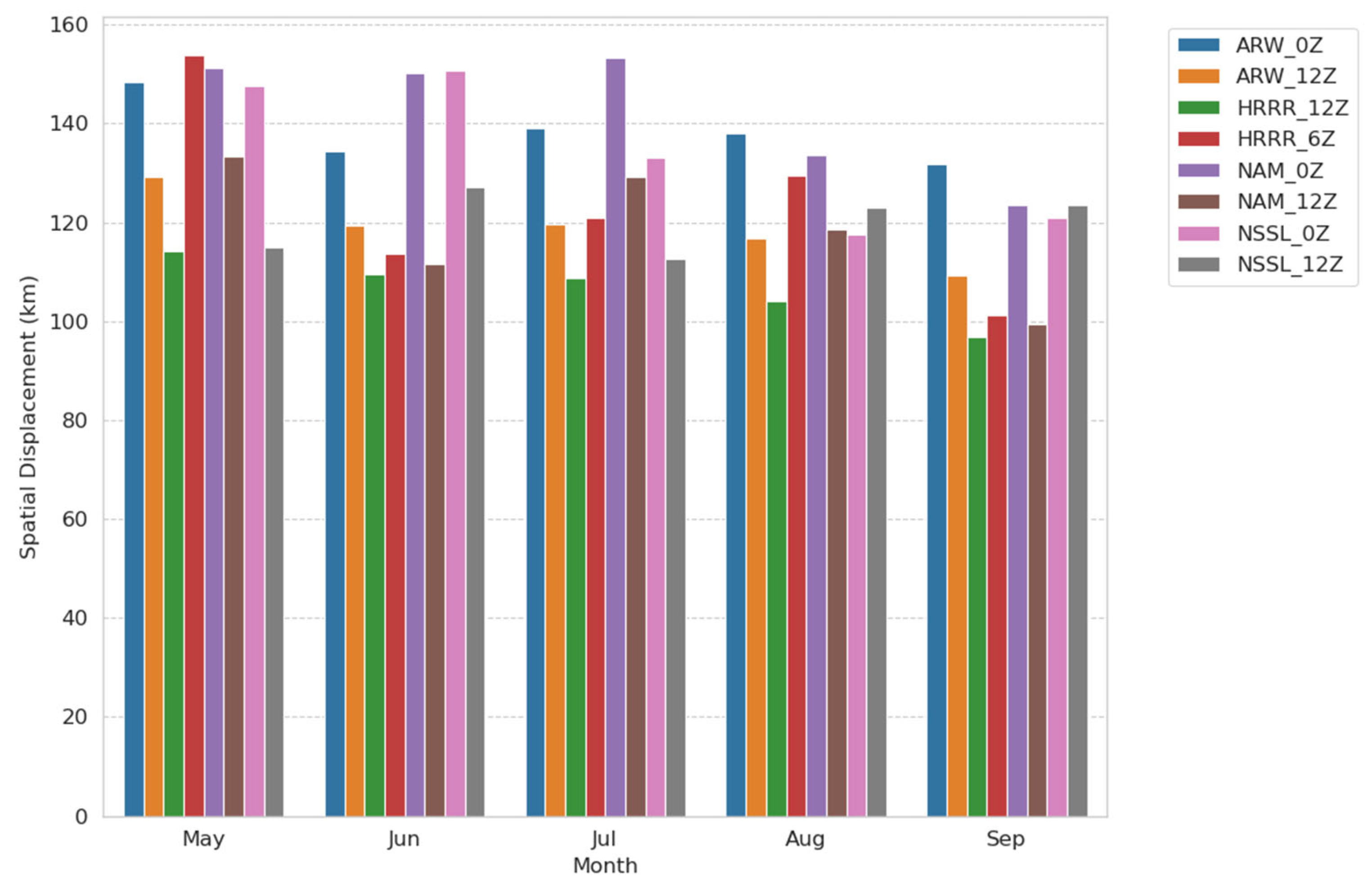
3.1. Displacement Errors
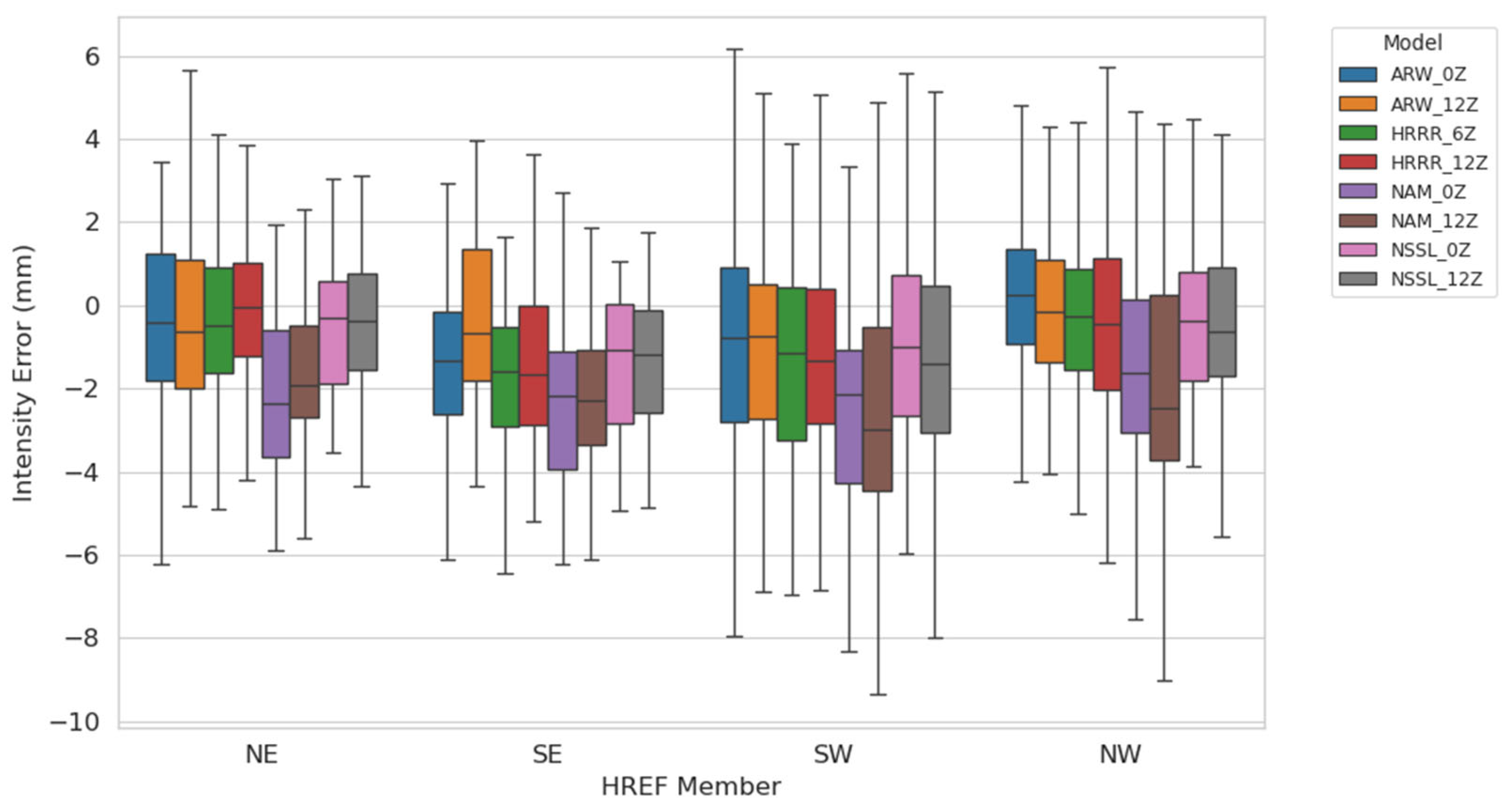
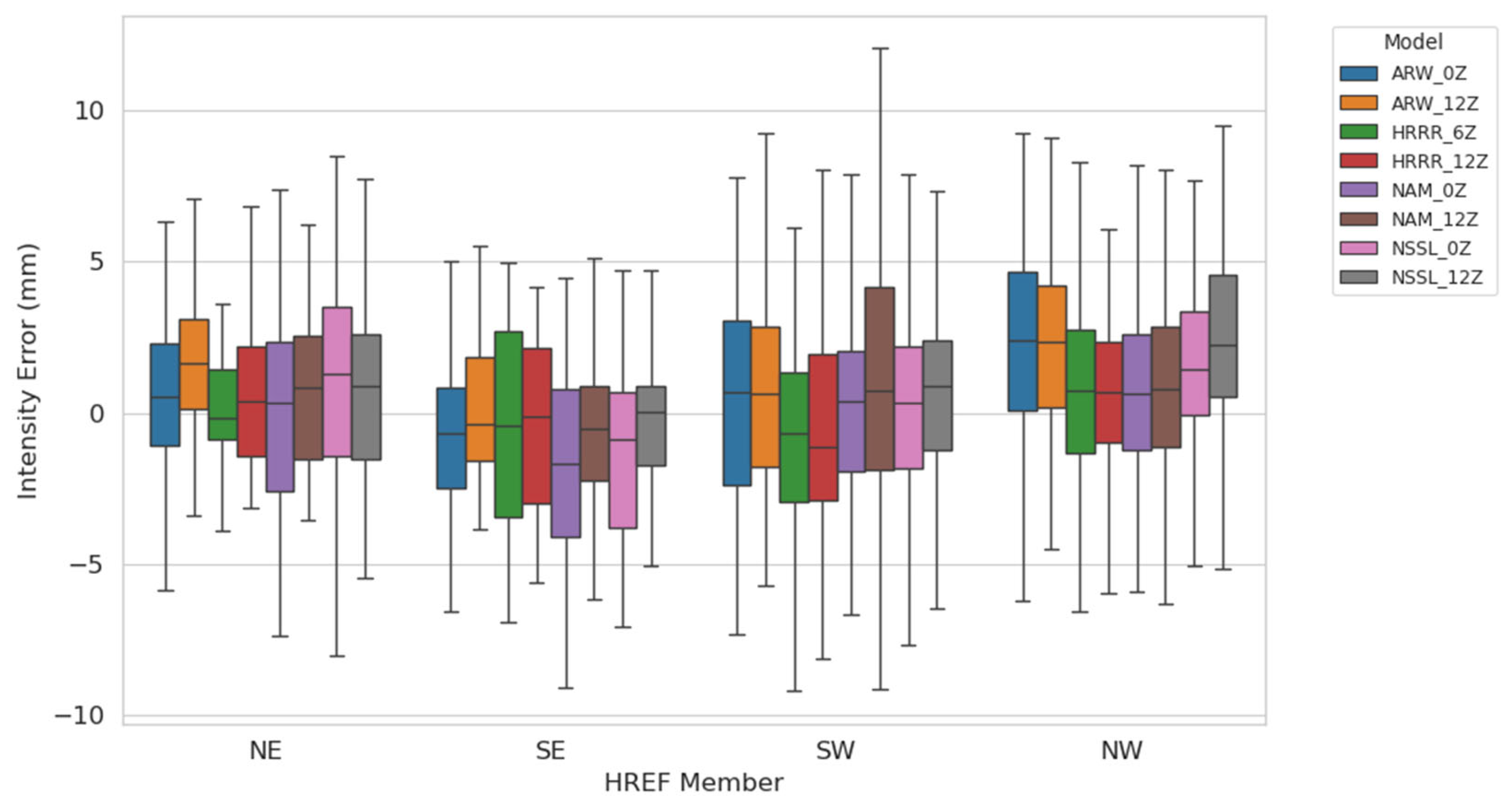
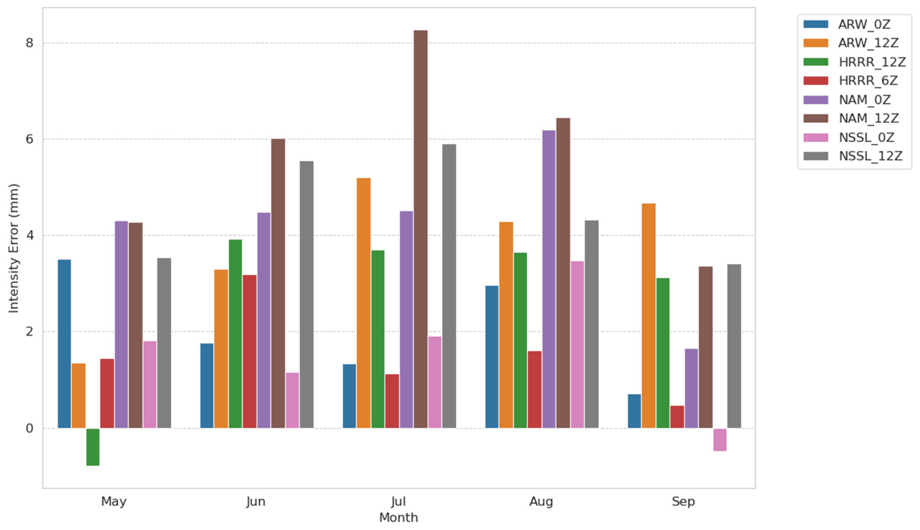
3.2. Intensity Errors
3.3. Water Volume and Area Errors
4. Discussion
5. Conclusions
Author Contributions
Funding
Data Availability Statement
Acknowledgments
Conflicts of Interest
References
- Ahmadalipour, A.; Moradkhani, H. A Data-Driven Analysis of Flash Flood Hazard, Fatalities, and Damages over the CONUS during 1996–2017. J. Hydrol. 2019, 578, 124106. [Google Scholar] [CrossRef]
- Cutter, S.L.; Emrich, C.T.; Gall, M.; Reeves, R. Flash Flood Risk and the Paradox of Urban Development. Nat. Hazards Rev. 2018, 19, 1–12. [Google Scholar] [CrossRef]
- Jirak, I.L.; Cotton, W.R.; McAnelly, R.L. Satellite and Radar Survey of Mesoscale Convective System Development. Mon. Weather Rev. 2003, 131, 2428–2449. [Google Scholar] [CrossRef]
- Stevenson, S.N.; Schumacher, R.S. A 10-Year Survey of Extreme Rainfall Events in the Central and Eastern United States Using Gridded Multisensor Precipitation Analyses. Mon. Weather Rev. 2014, 142, 3147–3162. [Google Scholar] [CrossRef]
- Hitchens, N.M.; Baldwin, M.E.; Trapp, R.J. An Object-Oriented Characterization of Extreme Precipitation-Producing Convective Systems in the Midwestern United States. Mon. Weather Rev. 2012, 140, 1356–1366. [Google Scholar] [CrossRef]
- Fritsch, J.M.; Kane, R.J.; Chelius, C.R. The Contribution of Mesoscale Convective Weather Systems to the Warm-Season Precipitation in the United States. J. Appl. Meteorol. Climatol. 1986, 25, 1333–1345. [Google Scholar] [CrossRef]
- Špitalar, M.; Gourley, J.J.; Lutoff, C.; Kirstetter, P.E.; Brilly, M.; Carr, N. Analysis of Flash Flood Parameters and Human Impacts in the US from 2006 to 2012. J. Hydrol. 2014, 519, 863–870. [Google Scholar] [CrossRef]
- Hugeback, K.K.; Franz, K.J.; Gallus, W.A. Short-Term Ensemble Streamflow Prediction Using Spatially Shifted QPF Informed by Displacement Errors. J. Hydrometeorol. 2023, 24, 21–34. [Google Scholar] [CrossRef]
- Adams, T.E., III; Dymond, R. The effect of QPF on real-time deterministic hydrologic forecast uncertainty. J. Hydrometeorol. 2019, 20, 1687–1705. [Google Scholar] [CrossRef]
- Seo, B.-C.; Quintero, F.; Krajewski, W.F. High-resolution QPF uncertainty and its implications for flood prediction: A case study for the Eastern Iowa flood of 2016. J. Hydrometeorol. 2018, 19, 1289–1304. [Google Scholar] [CrossRef]
- Olson, D.A.; Junker, N.W.; Korty, B. Evaluation of 33 Years of Quantitative Precipitation Forecasting at the NMC. Weather Forecast. 1995, 10, 498–511. [Google Scholar] [CrossRef]
- Fritsch, J.M.; Carbone, R.E. Improving Quantitative Precipitation Forecasts in the Warm Season: A USWRP Research and Development Strategy. Bull. Am. Meteorol. Soc. 2004, 85, 955–965. [Google Scholar] [CrossRef]
- Gallus, W.A., Jr. The Challenge of Warm-Season Convective Precipitation Forecasting. In Rainfall Forecasting; Wong, T.S.W., Ed.; Nova Science Publishers: Hauppauge, NY, USA, 2012; pp. 129–160. ISBN 978-61942-134-9. [Google Scholar]
- Keil, C.; Heinlein, J.; Craig, G.C. The convective adjustment time-scale as indicator of predictability of convective precipitation. Q. J. R. Meteorol Soc. 2014, 140, 480–490. [Google Scholar] [CrossRef]
- Wapler, K.; James, P. Thunderstorm occurrence and characteristics in Central Europe under different synoptic conditions. Atmos. Res. 2015, 158–159, 231–244. [Google Scholar] [CrossRef]
- Nielsen, E.R.; Schumacher, R.S. Using Convection-Allowing Ensembles to Understand the Predictability of an Extreme Rainfall Event. Mon. Weather Rev. 2016, 144, 3651–3676. [Google Scholar] [CrossRef]
- Stensrud, D.J.; Fritsch, J.M. Mesoscale Convective Systems in Weakly Forced Large-Scale Environments. Part II: Generation of a Mesoscale Initial Condition. Mon. Weather Rev. 1994, 122, 2068–2083. [Google Scholar] [CrossRef]
- Stensrud, D.J.; Fritsch, J.M. Mesoscale Convective Systems in Weakly Forced Large-Scale Environments. Part III: Numerical Simulations and Implications for Operational Forecasting. Mon. Weather Rev. 1994, 122, 2084–2104. [Google Scholar] [CrossRef]
- Gallus, W.A. Eta Simulations of Three Extreme Precipitation Events: Sensitivity to Resolution and Convective Parameterization. Weather Forecast. 1999, 14, 405–426. [Google Scholar] [CrossRef]
- Roberts, B.; Gallo, B.T.; Jirak, I.L.; Clark, A.J.; Dowell, D.C.; Wang, X.; Wang, Y. What Does a Convection-Allowing Ensemble of Opportunity Buy Us in Forecasting Thunderstorms? Weather Forecast. 2020, 35, 2293–2316. [Google Scholar] [CrossRef]
- Schwartz, C.S.; Kain, J.S.; Weiss, S.J.; Xue, M.; Bright, D.R.; Kong, F.; Thomas, K.W.; Levit, J.J.; Coniglio, M.C. Next-Day Convection-Allowing WRF Model Guidance: A Second Look at 2-km versus 4-km Grid Spacing. Mon. Weather Rev. 2009, 137, 3351–3372. [Google Scholar] [CrossRef]
- Kain, J.S.; Weiss, S.J.; Bright, D.R.; Baldwin, M.E.; Levit, J.J.; Carbin, G.W.; Schwartz, C.S.; Weisman, M.L.; Droegemeier, K.K.; Weber, D.; et al. Some Practical Considerations Regarding Horizontal Resolution in the First Generation of Operational Convection-Allowing NWP. Weather Forecast. 2008, 23, 931–952. [Google Scholar] [CrossRef]
- Clark, A.J.; Weiss, S.J.; Kain, J.S.; Jirak, I.L.; Coniglio, M.; Melick, C.J.; Siewert, C.; Sobash, R.A.; Marsh, P.T.; Dean, A.R.; et al. An Overview of the 2010 Hazardous Weather Testbed Experimental Forecast Program Spring Experiment. Bull. Am. Meteorol. Soc. 2012, 93, 55–74. [Google Scholar] [CrossRef]
- Thielen, J.E.; Gallus, W.A. Influences of Horizontal Grid Spacing and Microphysics on WRF Forecasts of Convective Morphology Evolution for Nocturnal MCSs in Weakly Forced Environments. Weather Forecast. 2019, 34, 1495–1517. [Google Scholar] [CrossRef]
- Gallus, W.A.; Harrold, M.A. Challenges in Numerical Weather Prediction of the 10 August 2020 Midwestern Derecho: Examples from the FV3-LAM. Weather Forecast. 2023, 38, 1429–1445. [Google Scholar] [CrossRef]
- Stelten, S.; Gallus, W.A. Pristine Nocturnal Convective Initiation: A Climatology and Preliminary Examination of Predictability. Weather Forecast. 2017, 32, 1613–1635. [Google Scholar] [CrossRef]
- Kiel, B.M.; Gallus, W.A.; Franz, K.J.; Erickson, N. A Preliminary Examination of Warm Season Precipitation Displacement Errors in the Upper Midwest in the HRRRE and HREF Ensembles. J. Hydrometeorol. 2022, 23, 1007–1024. [Google Scholar] [CrossRef]
- Kalina, E.A.; Jankov, I.; Alcott, T.; Olson, J.; Beck, J.; Berner, J.; Dowell, D.; Alexander, C. A Progress Report on the Development of the High-Resolution Rapid Refresh Ensemble. Weather Forecast. 2021, 36, 791–804. [Google Scholar] [CrossRef]
- Gallus, W.A. Application of Object-Based Verificaiton Techniques to Ensemble Precipitation Forecasts. Wea. Forecast. 2010, 25, 144–158. [Google Scholar] [CrossRef]
- Davis, C.A.; Brown, B.; Bullock, R. Object-Based Verification of Precipitation Forecasts. Part I: Application to Convective Rain Systems. Mon. Weather Rev. 2006, 134, 1785–1795. [Google Scholar] [CrossRef]
- Zhang, J.; Howard, K.; Langston, C.; Kaney, B.; Qi, Y.; Tang, L.; Grams, H.; Wang, Y.; Cockcks, S.; Martinaitis, S.; et al. Multi-Radar Multi-Sensor (MRMS) Quantitative Precipitation Estimation: Initial Operating Capabilities. Bull. Am. Meteorol. Soc. 2016, 97, 621–638. [Google Scholar] [CrossRef]
- Smith, T.M.; Lakshmanan, V.; Stumpf, G.J.; Ortega, K.L.; Hondl, K.; Cooper, K.; Calhoun, K.M.; Kingfield, D.M.; Manross, K.L.; Toomey, R.; et al. Multi-Radar Multi-Sensor (MRMS) Severe Weather and Aviation Products: Initial Operating Capabilities. Bull. Amer. Meteor. Soc. 2016, 97, 1617–1630. [Google Scholar] [CrossRef]
- Skamarock, W.C.; Klemp, J.B.; Dudhia, J.; Gill, D.O.; Barker, D.; Duda, M.G.; Powers, J.G. A Description of the Advanced Research WRF Version 3, NCAR Technical Note; National Center for Atmospheric Research: Boulder, CO, USA, 2008; p. 125. [Google Scholar]
- Janjic, Z.; Gall, R. Scientific Documentation of the NCEP Nonhydrostatic Multiscale Model on the B Grid (NMMB). Part 1 Dynamics; National Center for Atmospheric Research: Boulder, CO, USA, 2012; p. 75. [Google Scholar]
- Putman, W.M.; Lin, S.J. Finite-Volume Transport on Various Cubed-Sphere Grids. J. Comput. Phys. 2007, 227, 55–78. [Google Scholar] [CrossRef]
- Benjamin, S.G.; Weygandt, S.S.; Brown, J.M.; Hu, M.; Alexander, C.R.; Smirnova, T.G.; Olson, J.B.; James, E.P.; Dowell, D.C.; Grell, G.A.; et al. A North American Hourly Assimilation and Model Forecast Cycle: The Rapid Refresh. Mon. Weather Rev. 2016, 144, 1669–1694. [Google Scholar] [CrossRef]
- Zhou, X.; Juang, H.M.H. A Model Instability Issue in the National Centers for Environmental Prediction Global Forecast System Version 16 and Potential Solutions. Geosci. Model Dev. 2023, 16, 3263–3274. [Google Scholar] [CrossRef]
- Hong, S.Y.; Noh, Y.; Dudhia, J. A New Vertical Diffusion Package with an Explicit Treatment of Entrainment Processes. Mon. Weather Rev. 2006, 134, 2318–2341. [Google Scholar] [CrossRef]
- Hong, S.; Lim, J. The WRF Single-Moment 6-Class Microphysics Scheme (WSM6). J. Korean Meteorol. Soc. 2006, 42, 129–151. [Google Scholar]
- Thompson, G.; Field, P.R.; Rasmussen, R.M.; Hall, W.D. Explicit Forecasts of Winter Precipitation Using an Improved Bulk Microphysics Scheme. Part II: Implementation of a New Snow Parameterization. Mon. Weather Rev. 2008, 136, 5095–5115. [Google Scholar] [CrossRef]
- Nakanishi, M.; Niino, H. Development of an Improved Turbulence Closure Model for the Atmospheric Boundary Layer. J. Meteorol. Soc. Jpn. 2009, 87, 895–912. [Google Scholar] [CrossRef]
- Janjić, Z.I. The Step-Mountain Eta Coordinate Model: Further Developments of the Convection, Viscous Sublayer, and Turbulence Closure Schemes. Mon. Weather Rev. 1994, 122, 927–945. [Google Scholar] [CrossRef]
- Aligo, E.A.; Ferrier, B.; Jacob, R. Carley Modified NAM Microphysics for Forecasts of Deep Convective Storms. Mon. Weather Rev. 2018, 146, 4115–4153. [Google Scholar] [CrossRef]
- Mittermaier, M.P. Improving Short-range High-resolution Model Precipitation Forecast Skill Using Time-Lagged Ensembles. Q. J. R. Meteorol. Soc. 2007, 133, 1487–1500. [Google Scholar] [CrossRef]
- Nemenyi, P.B. Distribution-free Multiple Comparisons. Ph.D. Thesis, Princeton University, Princeton, NJ, USA, 1963. [Google Scholar]
- Friedman, M. A comparison of alternative tests of significance for the problem of m rankings. Ann. Math. Stat. 1940, 11, 86–92. [Google Scholar] [CrossRef]
- Fisher, R.A. Statistical Methods for Research Workers. In Breakthroughs in Statistics: Methodology and Distribution; Springer: New York, NY, USA, 1970; pp. 66–70. [Google Scholar]
- Tukey, J. Comparing individual means in the Analysis of Variance. Biometrics 1949, 5, 99–114. [Google Scholar] [CrossRef] [PubMed]
- Wade, A.R.; Jirak, I.L.; Lyza, A.W. Regional and Seasonal Biases in Convection-Allowing Model Forecasts of Near-Surface Temperature and Moisture. Weather Forecast. 2023, 38, 2415–2426. [Google Scholar] [CrossRef]
- Moore, B.J.; Mahoney, K.M.; Sukovich, E.M.; Cifelli, R.; Hamill, T.M. Climatology and Environmental Characteristics of Extreme Precipitation Events in the Southeastern United States. Mon. Weather Rev. 2015, 143, 718–741. [Google Scholar] [CrossRef]


| ARW_0 | ARW_12 | HRRR_12 | HRRR_6 | NAM_0 | NAM_12 | NSSL_0 | NSSL_12 | |
|---|---|---|---|---|---|---|---|---|
| ARW_0 | ||||||||
| ARW_12 | 0.978 | |||||||
| HRRR_12 | 0.884 | 0.284 | ||||||
| HRRR_6 | 0.228 | 0.015 | 0.959 | |||||
| NAM_0 | 0.001 | 0.045 | <0.001 | <0.001 | ||||
| NAM_12 | <0.001 | 0.002 | <0.001 | <0.001 | 0.984 | |||
| NSSL_0 | 0.994 | 1.000 | 0.401 | 0.029 | 0.024 | <0.001 | ||
| NSSL_12 | 0.316 | 0.905 | 0.008 | <0.001 | 0.630 | 0.120 | 0.819 |
| ARW_0 | ARW_12 | HRRR_12 | HRRR_6 | NAM_0 | NAM_12 | NSSL_0 | NSSL_12 | |
|---|---|---|---|---|---|---|---|---|
| ARW_0 | ||||||||
| ARW_12 | 0.819 | |||||||
| HRRR_12 | 0.915 | 0.112 | ||||||
| HRRR_6 | 0.138 | <0.001 | 0.860 | |||||
| NAM_0 | 0.819 | 1.000 | 0.112 | <0.001 | ||||
| NAM_12 | 0.366 | 0.997 | 0.014 | <0.001 | 0.997 | |||
| NSSL_0 | 0.884 | 0.090 | 1.000 | 0.895 | 0.090 | 0.010 | ||
| NSSL_12 | 0.987 | 0.999 | 0.383 | 0.009 | 0.999 | 0.905 | 0.332 |
Disclaimer/Publisher’s Note: The statements, opinions and data contained in all publications are solely those of the individual author(s) and contributor(s) and not of MDPI and/or the editor(s). MDPI and/or the editor(s) disclaim responsibility for any injury to people or property resulting from any ideas, methods, instructions or products referred to in the content. |
© 2025 by the authors. Licensee MDPI, Basel, Switzerland. This article is an open access article distributed under the terms and conditions of the Creative Commons Attribution (CC BY) license (https://creativecommons.org/licenses/by/4.0/).
Share and Cite
Gallus, W.A., Jr.; Duhachek, A.; Franz, K.J.; Frazier, T. A Climatology of Errors in HREF MCS Precipitation Objects. Water 2025, 17, 2168. https://doi.org/10.3390/w17152168
Gallus WA Jr., Duhachek A, Franz KJ, Frazier T. A Climatology of Errors in HREF MCS Precipitation Objects. Water. 2025; 17(15):2168. https://doi.org/10.3390/w17152168
Chicago/Turabian StyleGallus, William A., Jr., Anna Duhachek, Kristie J. Franz, and Tyreek Frazier. 2025. "A Climatology of Errors in HREF MCS Precipitation Objects" Water 17, no. 15: 2168. https://doi.org/10.3390/w17152168
APA StyleGallus, W. A., Jr., Duhachek, A., Franz, K. J., & Frazier, T. (2025). A Climatology of Errors in HREF MCS Precipitation Objects. Water, 17(15), 2168. https://doi.org/10.3390/w17152168