Development of Open-Source Tools for Event-Based Hydrological Modelling Using GIS and Python

Abstract

Detailed modelling of water dynamics at the catchment is of paramount importance for the optimal management and allocation of water resources. The main objective of this work is to present a set of QGIS-based routines for processing easily available geographical information to deliver inputs for integration into hydrological models developed in the Python environment. We present QGIS processes that deliver open format exchangeable files with physical information required for hydrological modelling, allowing a better tailoring of hydrological modelling tasks compared to other blinded existing models. We present the general framework by processing spatial information and running a set of hydrological models in different cases studies in the Spanish Ebro River basin, proving the utility of the proposed method for applying complex and tailored hydrological simulations.

1. Introduction

Hydrological models play a key role in the proper management of water resources [1,2,3]. From the evaluation of management strategies [4,5,6] to the assessment and allocation of water resources [7,8] through the optimization of networks [9,10] or the assessment of the impact of climate change on water resources [11,12], hydrological models are essential across a wide range of water-related topics.

Hydrological models have evolved from simple tools with a few parameters to complex models requiring extensive geographical and meteorological information. The development of Geographical Information Systems (GIS) coupled with improvements in computational capabilities marked a step forward in hydrological modelling by enabling large-scale distributed simulations of time-dependent processes within the catchment. In parallel, the growing availability of remote sensing products has further enhanced the use of GIS in hydrological modelling, providing significant advantages over traditional on-site measurements by covering large areas with high spatio-temporal resolution, facilitating the simulation of dynamic hydrological phenomena with frequent updates. Scientists have largely used satellite images at different hydrological planes, for example, to estimate soil water content [13,14,15,16,17], evapotranspiration [18,19,20,21], streamflow [22,23,24,25,26,27] or precipitation [28,29,30,31,32,33].

Hydrologists have also exploited GIS to develop tools for complex hydrological simulations (see for example [25,34,35]) integrating models of different phenomena (often rainfall generation, infiltration/runoff and surface runoff flooding) into comprehensive packages with diverse functionalities (see for example SWAT or SWMM models). Most of these models utilise geographical information by either discretising the catchment into cells or aggregating data into homogeneous units (lumped models). They incorporate mathematical theories for simulating the processes while requiring users to provide spatial information (land use, topography, soil moisture or soil physical properties), which is pre-processed prior to its incorporation into the models, along with the parameters required for the selected hydrological simulations.

Such tools do not provide users with full access to the internal models and routines, limiting the ability to adjust the geographic information, mathematical formulations or model architecture. This may hinder the development of tailored applications and also limit the level of generality often sought by researchers. Hydrological models are complex and frequently require case-specific and tailored analysis to deliver accurate results, or even on many occasions to ensure the convergence of mathematical routines.

In contrast to proprietary solutions, open-paradigm tools, such as QGIS and Python, offer the required flexibility and adaptability to overcome the previous limitations. Using these tools, tailored models and routines can be developed to perform highly-specific and complex hydrological analyses. In this work, we leverage these tools to provide a methodological framework for analysing event-based hydrological processes at the catchment scale. Building on this approach, the main objective of this paper is to present a methodology for coupling Python programming tools with spatial data generated from QGIS outputs to execute hydrological simulations. Since the aim of this manuscript is to demonstrate the applicability of the GIS−Python framework for spatial data processing, we will present several applications of the proposed framework to specific hydrological models using different pilot catchments within the Spanish Ebro River basin.

2. Materials and Methods

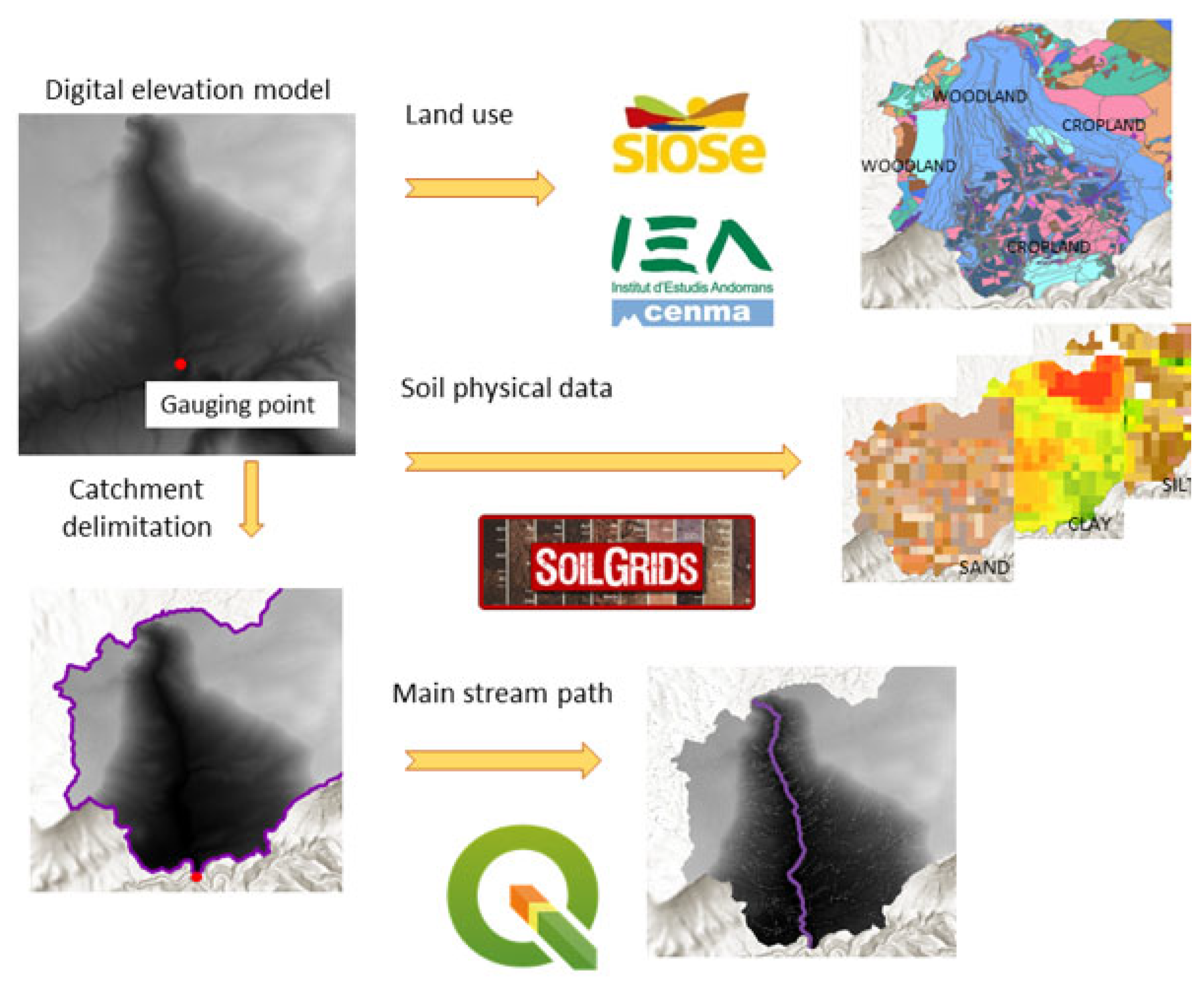
In this section, we first present a general overview of the tasks performed in QGIS 3.10 Coruña (Section 2.1), a description of the integration with hydrological modelling (Section 2.2), while the last section presents the case study we used as a matter of example (Section 2.3).

2.1. GIS Operations

Figure 1 sketches the overall implementation of the model, and

Table 1. List of models, inputs, outputs and used tools.

Steps	Inputs	Outputs	Tools
Catchment delineation Model: 1. Catchment_delimitation	DEM rasters, coordinate reference system (CRS), minimum size of watershed and gauging point	DEM_mosaic (raster), drainage_direction (raster), stream_segments (raster) and catchment area (raster)	QGIS (raster pixel to points, clip, distance to the nearest hub, extract by expression), GDAL (merge, translate), GRASS (r.watershed, r.water.outlet and r.to.vect)
Topography and land use Model: 2. Topographical_factors_and_land_use	Catchment (raster), CRS, DEM_mosaic (Raster), Land use source (polygon), stream_segments (raster)	Catchment (polygon vector layer), Elevation (Raster), Slope (Raster), Land_use (Polygon—vector—and raster), stream_segments (vector)	QGIS (dissolve, slope, clip and raster layer properties), GDAL (translate, olygonise and rasterise), GRASS (r.mask.vect)
Spatial homogenisation Model: 3. Resampling_SOILGRIDS_ variables	Sand, silt, clay, soil classes and bulk density SOILGRIDS rasters and elevation (raster)	Sand, silt, clay, soil classes and bulk density resampled (raster)	QGIS (minimum bounding geometry, buffer and raster layer properties), GDAL (warp), GRASS (r.resample)
Flow pathways Model: 4. Shortest_ path Catchment characterisation Model: 5. Catchment_ characterisation	Stream_segments (vector), start point and end point Catchment (polygon), slope (raster), Land_use (raster) and shortest path length (vector)	Shortest_path (vector line layer) Catchment_characteristics (polygon vector)	QGIS (shortest path point to point) QGIS (zonal statistics, field calculator)
Exchangeable files Model: 6. ASCII_ conversion	Catchment, land use, elevation, slope, sand, silt, clay, soil class and bulk density (raster layers)	Catchment, land use, sand, silt, clay, soil class and bulk density (.asc file)	GRASS (r.aout.ascii)

DEM—digital elevation model; CRS—coordinate reference system; GDAL—Geospatial Data abstraction library; GRASS—Geographic Resources Analysis Support System; ASCII—American Standard Code for Information Interchange.

shows the modelling tools that structure the proposed methodology.

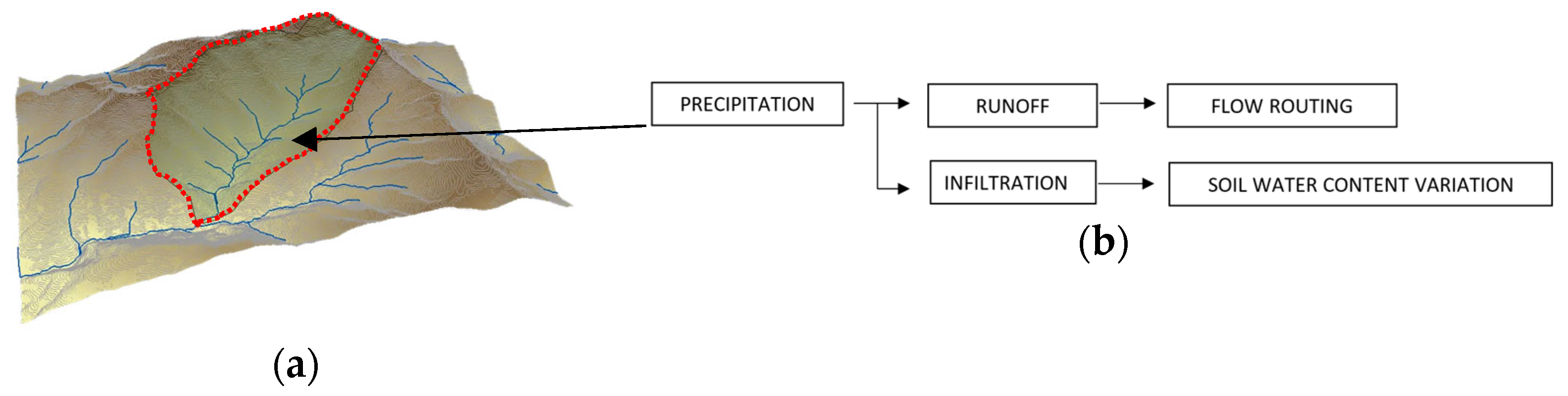
2.2. Integration with Hydrological Models

To develop the tools presented in this paper, we simulated some event-based (rainfall-runoff) hydrological processes based on the mass conservation law, with infiltration/abstraction and flow routing as the main processes involved. Although specific details depend on the selected theories, such simulations require gathering and processing spatial information related to the following:

• Land uses, soil physical properties and soil moisture influencing infiltration/abstractions generation.
• Topographical information for delineating catchments and determining the transient time and flow routing downstream.

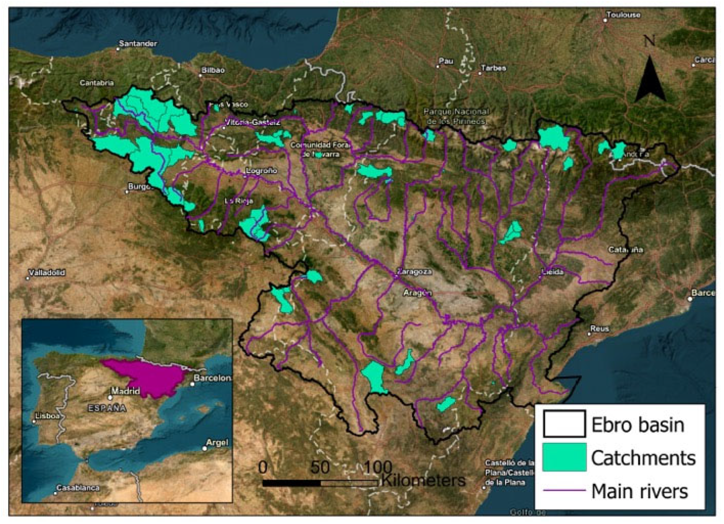
Our general approach follows two consecutive steps: (1) collecting and pre-processing spatial information; and (2) transforming it to deliver exchangeable information to feed hydrological models.

The QGIS routines delivered the catchment’s specific information through either nD matrix-type (spatial information such as land uses, soil physical properties or soil moisture) or 1D array (mainstream length, slope, entire area and area by land uses) formats in plain text files. From the QGIS outputs we obtained the information required for parametrising the models we present in this section.

For the hydrological simulations we present in this manuscript, we assume the rainfall-runoff events within a catchment have to satisfy the mass conservation law expressed as Equation (1):

$${\displaystyle \frac{dS}{dt}}=I\left(t\right)-O(t)$$

(1)

where the difference between inputs (I(t)) and outputs (O(t)) produces the system internal variations dS/dt. However, the variables involved in rainfall-runoff processes depend on the time-scale we consider. When considering short-latency events, the inputs and outputs are precipitation and water discharge at the catchment’s downstream end point and the soil moisture variation represents the system internal variation.

For the specific case, we present in this manuscript focused on event-based hydrology, Equation (1) can be described as follows (Equations (2) and (3)):

$${\displaystyle \frac{dS}{dt}}=P\left(t\right)-R\left(t\right)-ET\left(t\right)$$

(2)

$$P\left(t\right)=Inf\left(t\right)+R\left(t\right)$$

(3)

where S [L] is the soil water storage, P(t) [L] is the precipitation at time t, Inf(t) [L] is the infiltration at time t, R(t) [L] is the runoff at time t, and ET(t) [L] is the evapotranspiration at time t. In this manuscript, we focus on short-term storm events with a duration of less than one hour. In this context, evapotranspiration can be neglected due to its expected small magnitude compared to the precipitation volumes.

Figure 2 represents an idealised catchment and the processes’ workflow we follow for the hydrological simulations.

We present some examples using the outputs of the QGIS operations for running the following: (1) the Green and Ampt [36] infiltration model (see Equations (2) and (3)) to estimate the excess of runoff from a set of synthetic storm events; (2) the soil conservation service curve number (see Equations (3)–(5)); and (3) the flow routing as estimated by the kinematic wave model integrated with the Muskingum-Cunge routine [37] (see Equations (6) and (7)). We code the models in Python 3.7.

Following Chow et al. [38], the Green-Ampt model provides the potential infiltration rate f(t) [L·T⁻¹] as given by Equations (4) and (5):

$$f\left(t\right)\cong k_s\left(1+{\displaystyle \frac{{\tau }_f·\Delta \theta }{F\left(t\right)}}\right),$$

(4)

$$F\left(t\right)=k_s·t+{\tau }_f·\Delta \theta ·Ln\left(1+{\displaystyle \frac{F\left(t\right)}{{\tau }_f·\Delta \theta }}\right)$$

(5)

where ks [L·T⁻¹], Δθ [L³·L⁻³] and τ_f [L] stand for the saturated hydraulic conductivity, the difference between the saturated and the initial soil water content and the wetting front suction head, respectively. This model requires a homogeneous soil with a uniform initial water content while the saturated wetting front is assumed to move downwards as a single piston-like displacement.

Similarly, the excess of runoff (E [L]) generated by a P [L] volume rainstorm depends on the curve number (CN, dimensionless) and the initial abstraction (Ia [L]) as follows (Equations (6)–(8)):

$$S=25.4 \ast \left({\displaystyle \frac{1000}{CN}}-10\right),$$

(6)

$$I_a=0.2 \ast S,$$

(7)

$$E={\displaystyle \frac{{\left(P-I_a\right)}^2}{P-I_a+S}}$$

(8)

The model assumes the precipitation above a given threshold (Initial abstraction) is divided between infiltration and runoff.

The kinematic wave method is given by Equations (9) and (10):

$${\displaystyle \frac{\partial Q}{\partial t}}+c{\displaystyle \frac{\partial Q}{\partial x}}=0$$

(9)

$$S_f=S_0$$

(10)

where Q ([L³·T⁻¹], x [L] and t [T] stand for the discharging flow over time t and across x, c [L·T⁻¹] is the wave celerity, and S₀ [L·L⁻¹] and Sf [L·L⁻¹] are the channel slope and the energy gradient, respectively. The kinematic wave solution for the Saint-Venant equations implies the flow is uniform, and the friction slope is approximately equal to the slope of the channel. For the Muskingum-Cunge [37] method, we followed the solutions presented in [38], solving the equations using an explicit finite difference approach with different time steps, setting Courant’s relationship between time and spatial steps to ensure convergence.

2.3. Case Study

We selected a set of 29 small-sized catchments at the Spanish Ebro River basin (see Figure 3). The Ebro River basin, located in Northeastern Spain, is the country’s largest river basin, covering approximately 85,000 km². Hydrologically, the Ebro River flows over 910 km from its headwaters in the Cantabrian Mountains to its delta on the Mediterranean Sea, with a complex network of tributaries exhibiting diverse flow regimes influenced by snowmelt, rainfall and groundwater contributions. Geologically, the basin is characterised by a combination of the Pyrenean ranges to the north, the Iberian System to the south, and the Ebro Depression in the central sector, which is filled with Tertiary and Quaternary sedimentary deposits, mainly clays, marls, and limestones, influencing infiltration rates and groundwater dynamics. Climatologically, the basin exhibits high variability, with Atlantic influences in the headwaters, a continental semi-arid climate in the central depression, and Mediterranean influences near the delta. The average annual precipitation ranges from over 1200 mm in the Pyrenean headwaters to less than 400 mm in the central valley, while average temperatures vary significantly, with cold winters and hot, dry summers dominating the lower basin.

We selected pilot catchments with high latency precipitation and water level records at the downstream end point, featuring homogeneous land uses and potential for easy parametrisation to apply hydrological models.

Table 2. Main properties of the selected catchments.

Catchment	z Max (masl)	z Min (masl)	Channel Length	Catchment Area
Aragón at Canfranc	2160.03	1041.91	18,987.66	18,254,694
Bailin at Sabiñanigo	1078.86	743.675	4651.442	4,508,212
Cidacos at Arnedillo	1607.32	647.671	28,141.38	176,407,587
Cidacos at Yanguas	1607.32	943.343	26,049.78	230,120,488
Deza at EmbidDeAriza	1091.97	780.169	40,193.02	207,366,324
Flamisell at Cabdella	2670.56	1275.38	17,336.71	72,034,834
Garona at Bossost	2577.25	710.235	47,696.3	440,715,489
Isuela at Trasobares	1580.56	636.852	28,743.83	116,994,476
Izalzu at Anduña	1501.12	796.684	12,066.23	47,171,880
Larraun at Iribas	697.602	560.652	3067.464	5,825,444
Nela at Villarcayo	1495.34	1065.76	16,309.96	105,146,261
Linares at SanPedroManrique	947.97	593.783	51,586.01	254,733,836
Oca at Oña	1235.93	572.718	90,988.14	1,038,283,932
Oja at Azurrulla	1895.08	919.251	14,463.59	73,822,908
Omecillo at Berengueda	940.005	477.69	37,291.6	342,161,356
Oroncillo at Oron	1031.87	477.678	39,005.88	215,597,179
Pancrudo at Navarrete	1301.75	899.522	46,608.72	381,876,679
Rudron at Valdelateja	971.635	651.205	50,960.24	505,378,148
Sanguesa at Onsella	1104.98	408.293	57,150.27	233,627,436
Subialde at Larrinoa	976.08	593.27	9730.708	21,360,782
Tiron at SanMiguelPedroso	1943.81	805.105	27,491.29	190,327,545
Trueba at MedinaDePomar	1361.59	578.945	53,004.09	468,549,100
Ubagua at Riezu	1212.42	491.038	91,333.75	35,536,916
Urederra at Barindano	736.78	500.118	6083.276	37,063,648
Urriobi at Espinal	1347.52	856.52	11,611.5	4,846,596
Vallfarrera at Alins	2601.49	1071.4	20,319.19	82,741,803
Veral at Zuriza	2093.41	1188.19	12,843.68	46,176,842
Zatoya at Ochagavia	1175.03	789.745	20,686.8	72,702,728
Zidacos at Garinoiain	636.188	485.35	7164.723	27,097,980

presents the main catchments characteristics.

Table 3. GIS data sources and spatial resolution.

Material	Pixel Resolution
Digital elevation model (DEM)	5 m
SoilGrids: silt, sand, clay and bulk density	250 m
Spanish Land Use System (SIOSE)	Polygon shapefile (minimum polygon size: 1 m2).

presents a summary of the GIS data sources used in this study, along with their respective spatial resolutions.

3. Results and Discussion

3.1. GIS-Based Processes

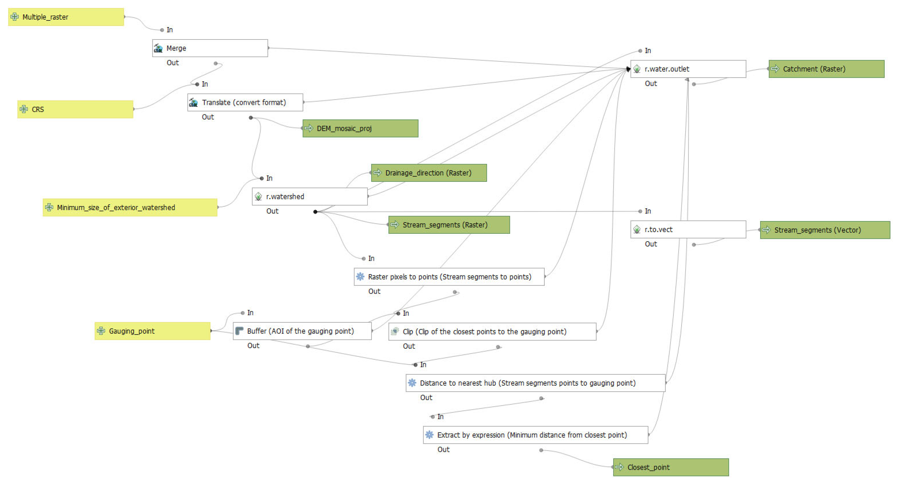
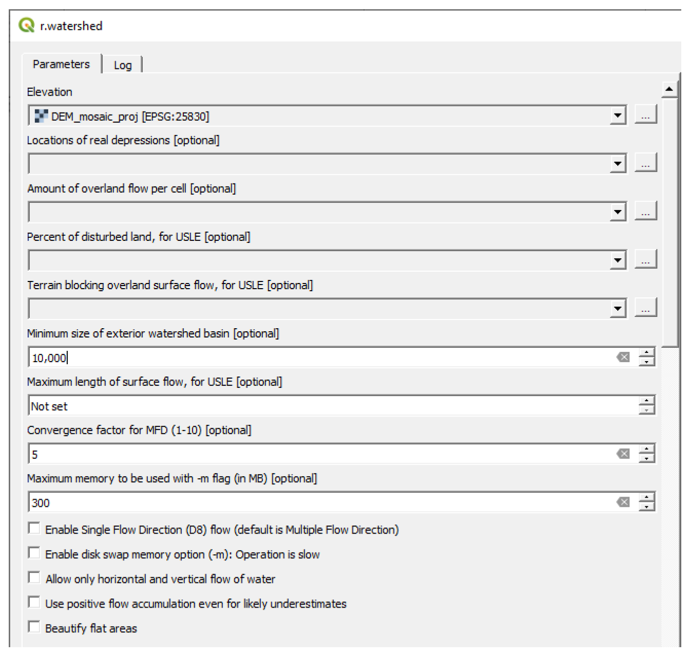
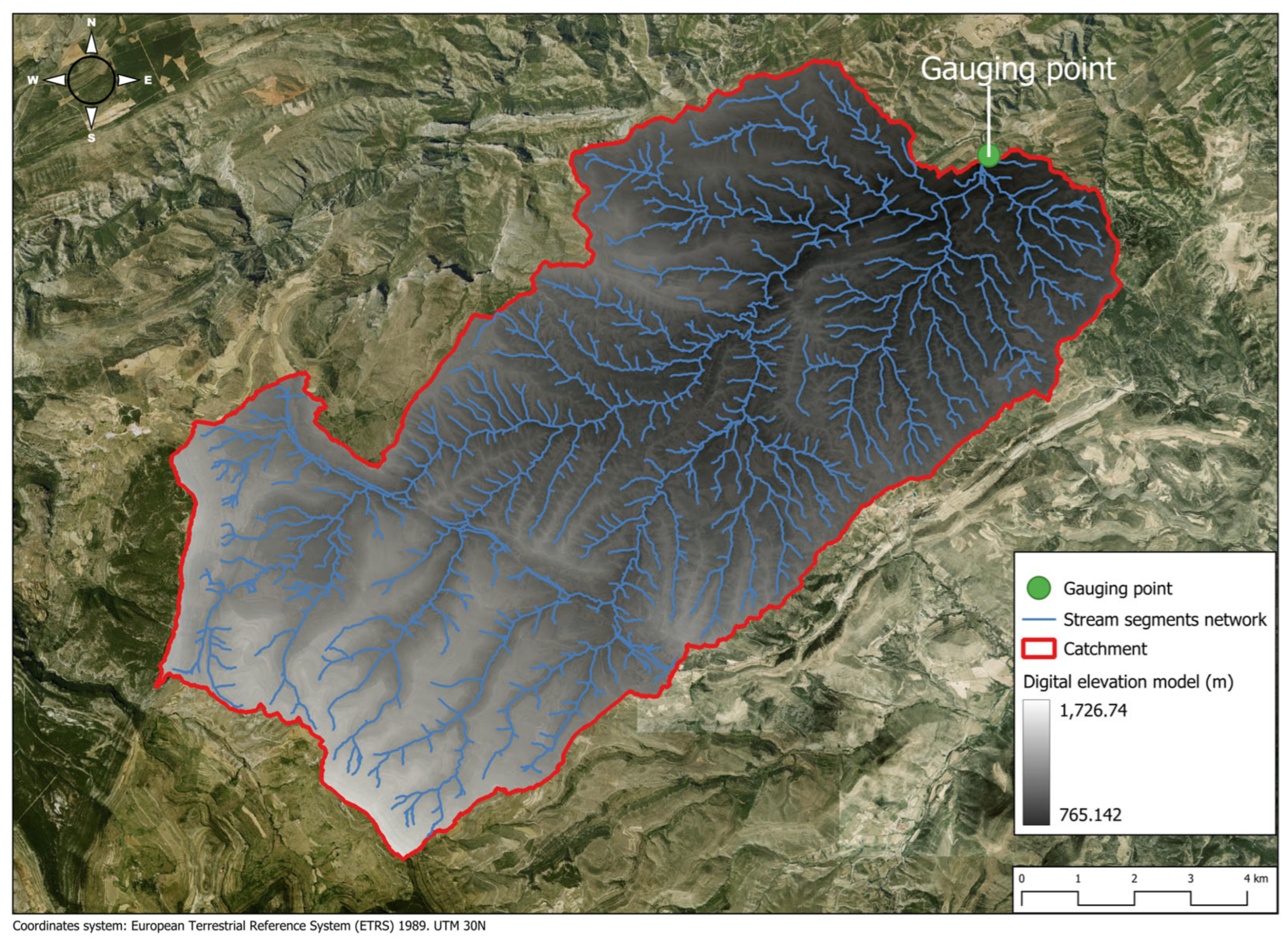
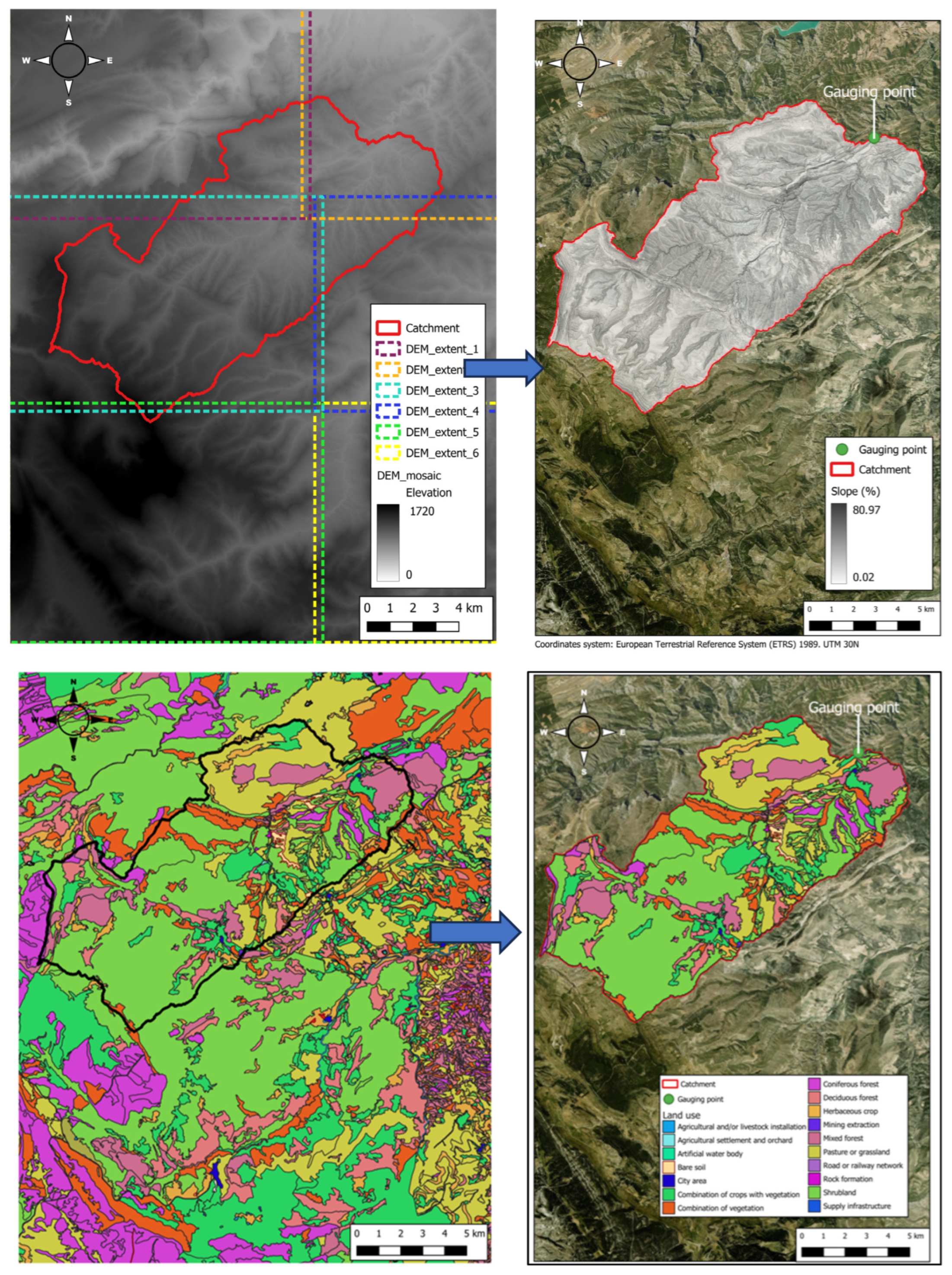
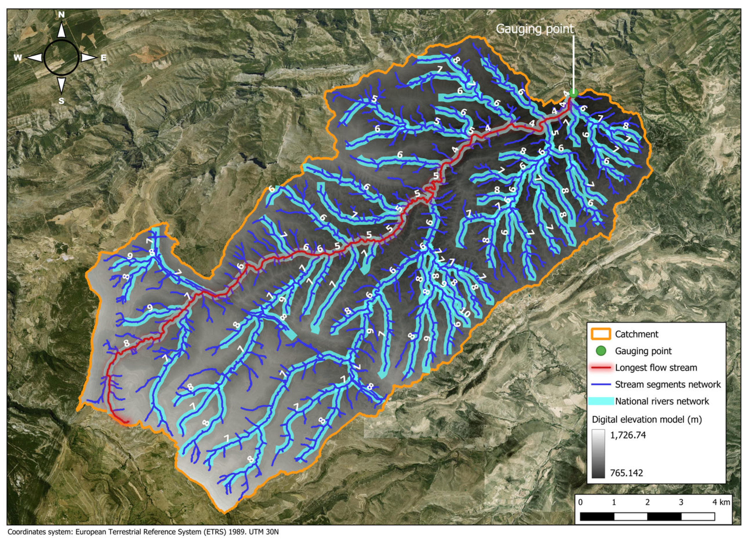
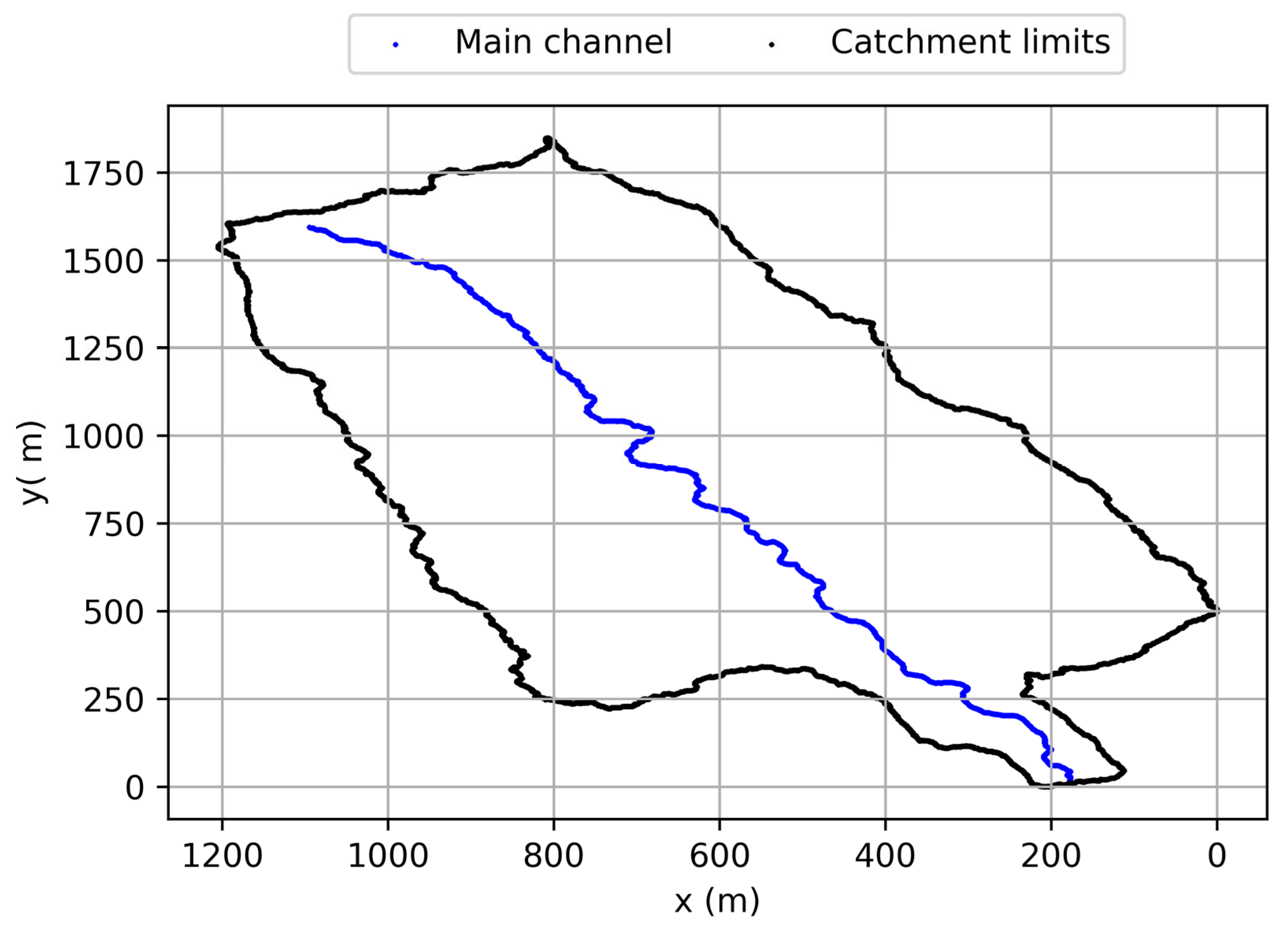
3.1.1. Catchment Delineation

We delineated the basins from the point where the water level gauge was placed. Figure 4 presents the QGIS flowchart displaying the processes and files involved.

The combination of the QGIS GRASS r.watershed and r.water.outlet toolbox algorithms enabled the definition of the catchment boundaries. We first ran the r.watershed tool using the DEM, setting the minimum watershed basin size equal to the DEM pixel size. From the catchment’s downstream endpoint (manually defined using the stream segments layer generated by r.watershed), the tool delineated the catchment boundaries based on the drainage direction layer produced by r.watershed. We used a DEM provided by the Spanish National Geography Institute (Instituto Geográfico Nacional, 2023) with a spatial resolution of 2 m. Figure 5 presents the parameter tuning used for both processes, while Figure 6 shows the resulting outputs.

Computing time became a relevant concern when using large DEM extents with a small pixel size. We obtained the coordinates of the water level gauging point and the DEM from different sources, which introduced spatial inconsistencies, as the gauging point was occasionally located far from the stream segment. This required us to manually define the catchment outlet point (see Figure 7). Additionally, we encountered several issues when exporting the data to raster layers, as empty raster files were occasionally generated during the modelling process. This likely resulted from corrupted internal routines, as the issue occurred randomly without an apparent cause.

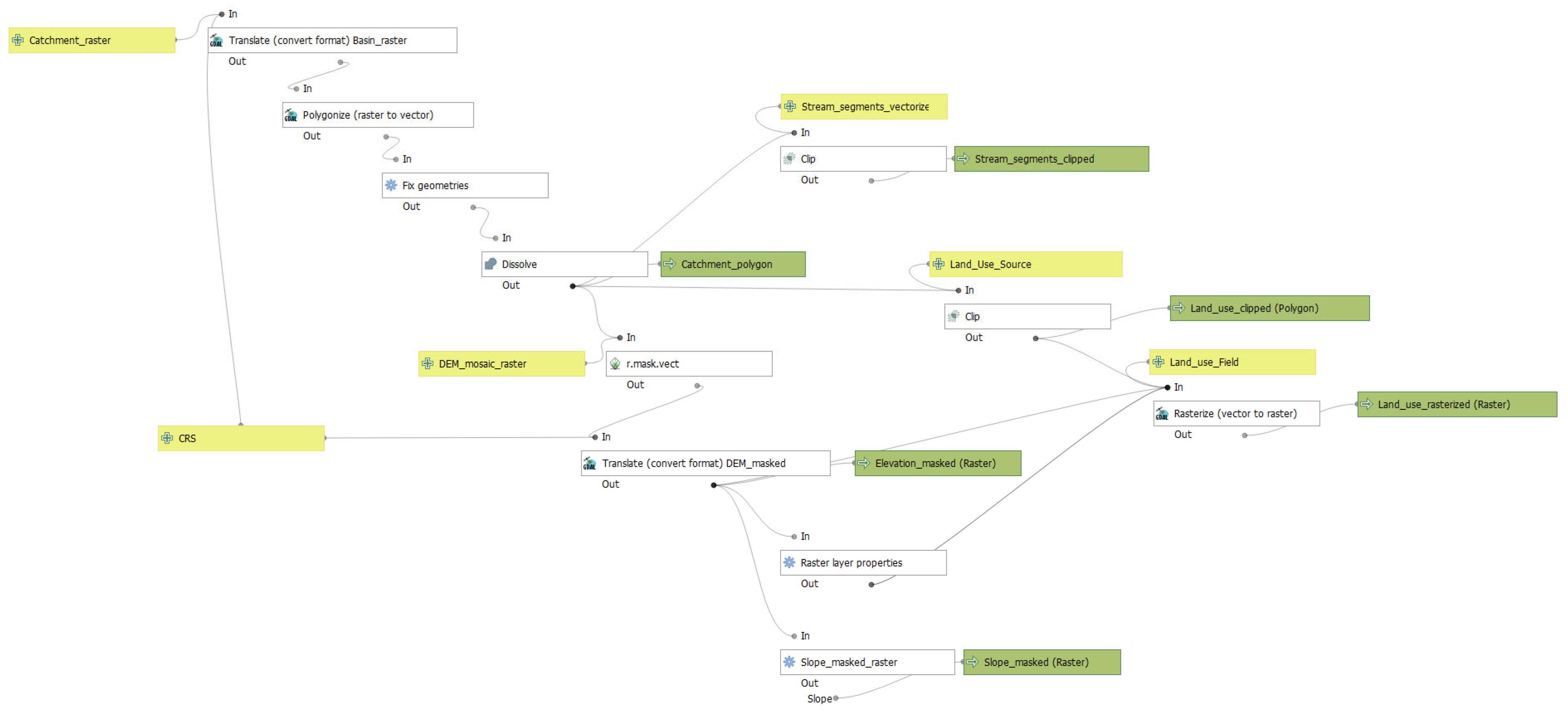
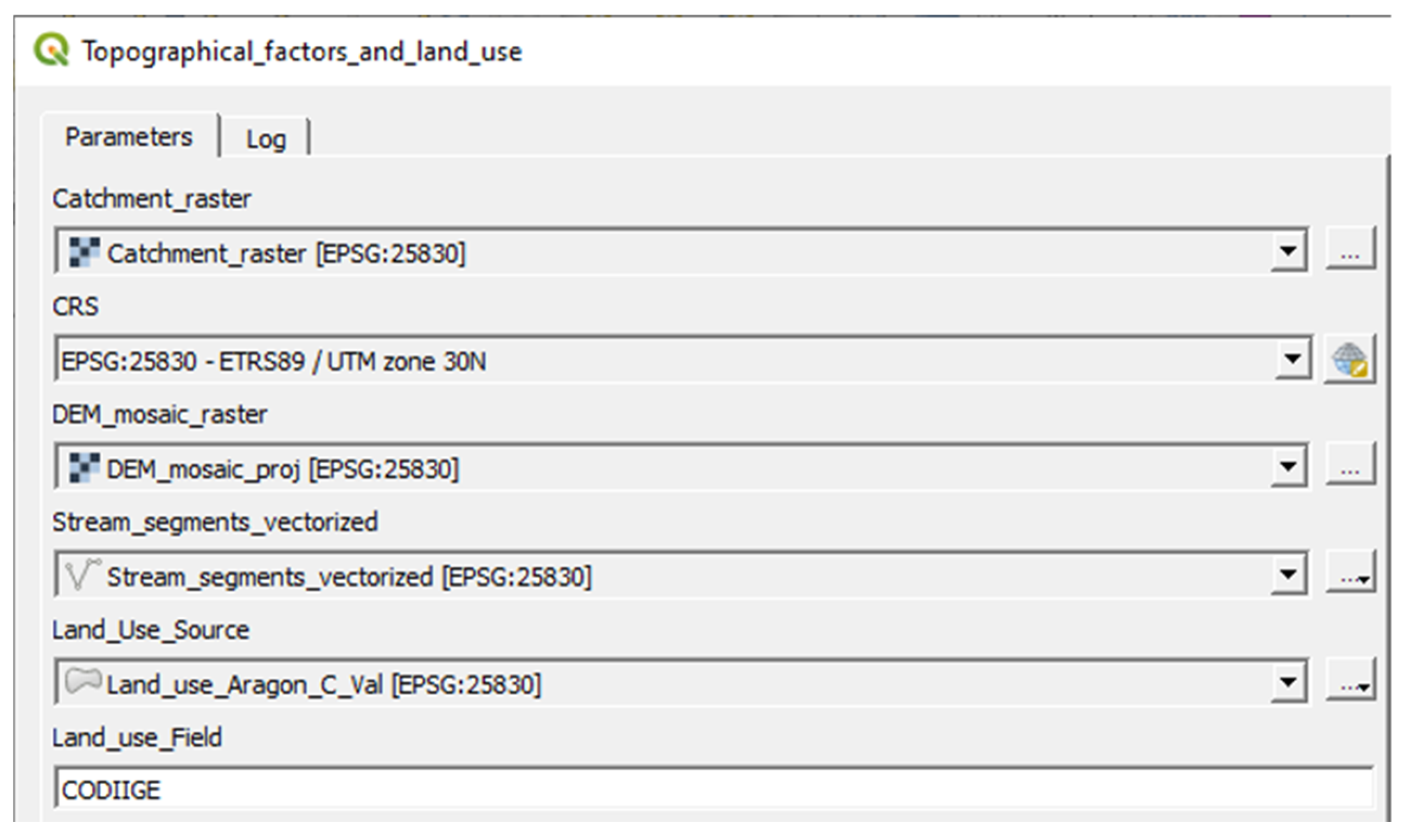
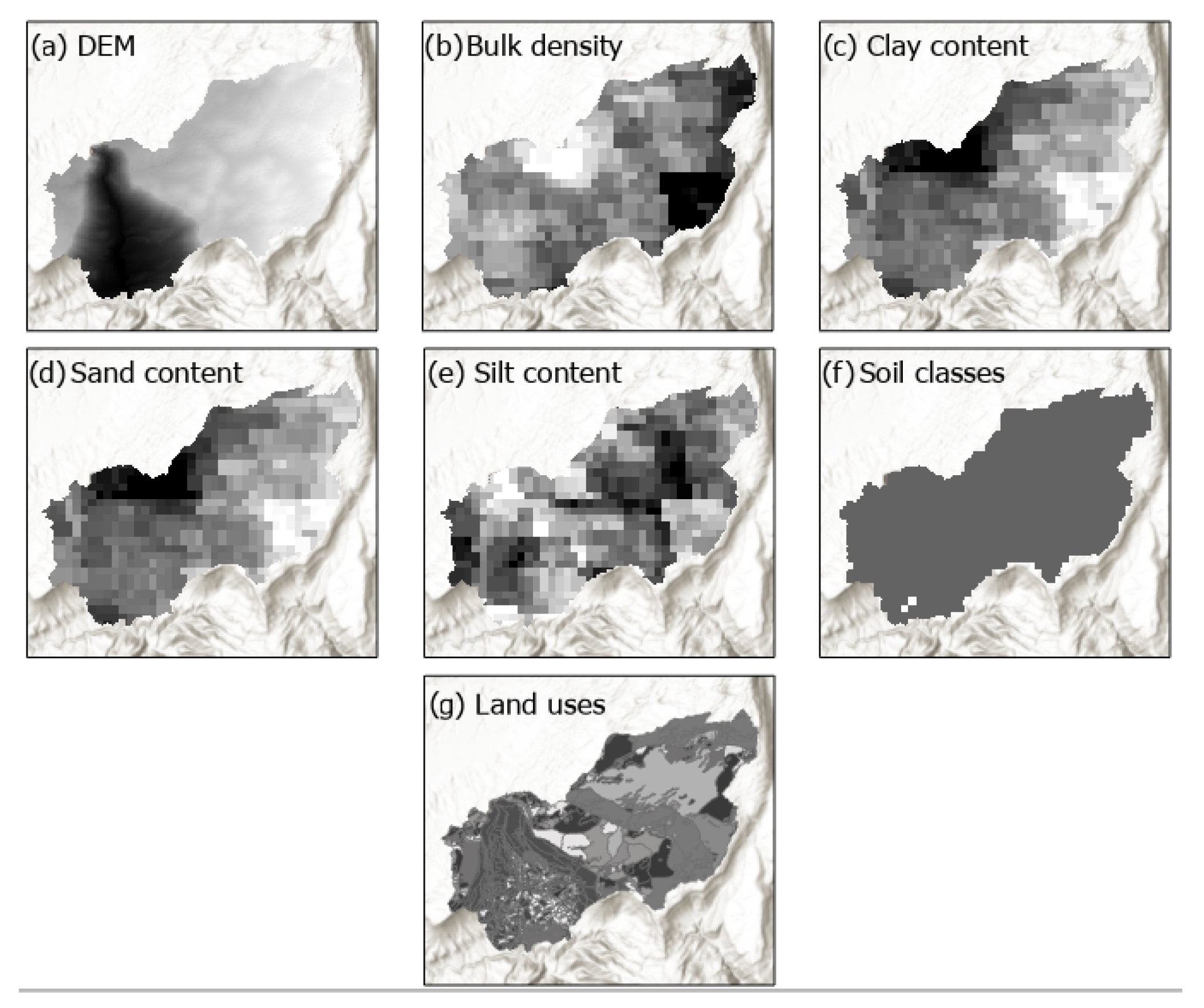
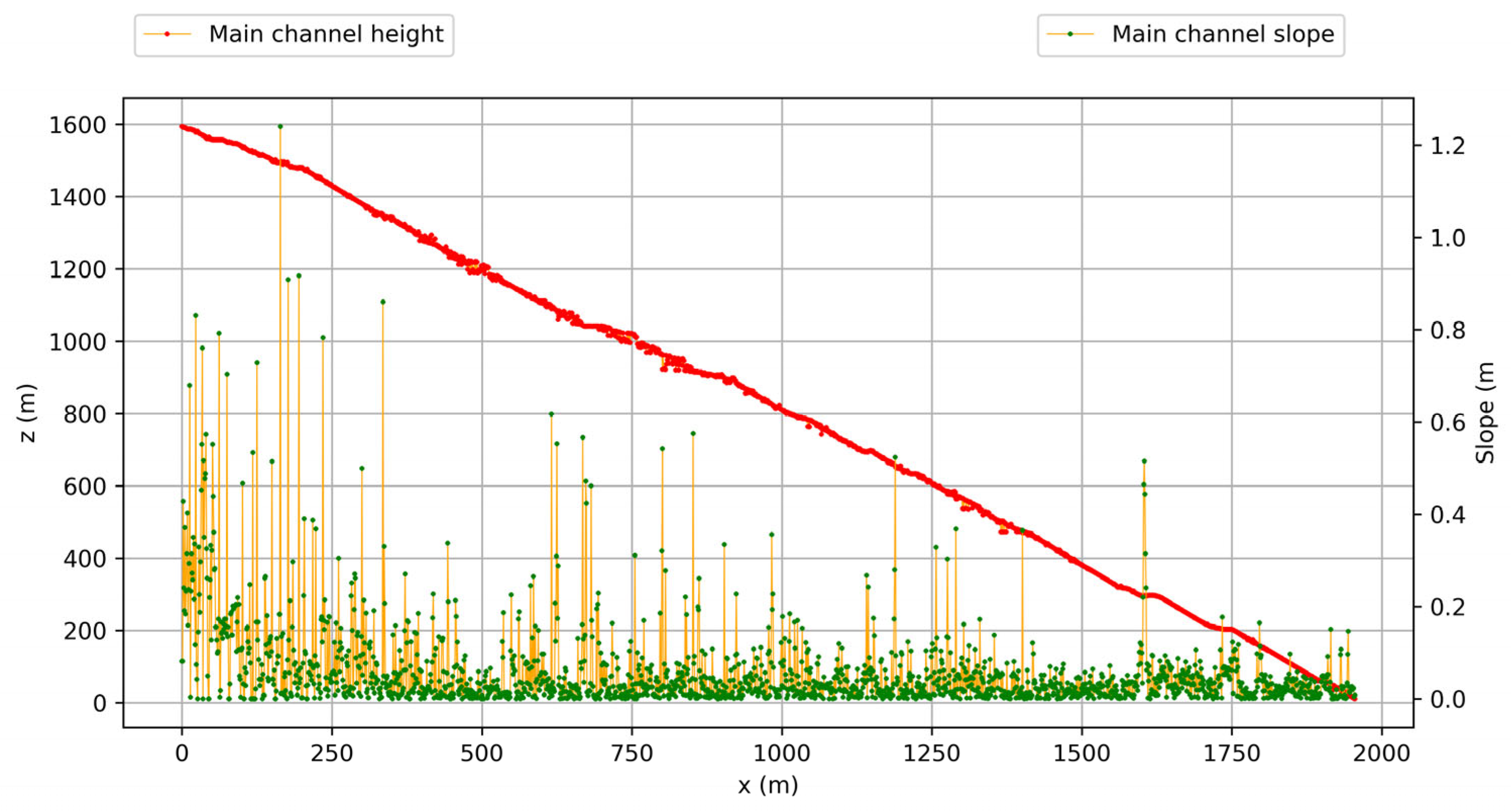
3.1.2. Topography and Land Uses

Once the catchment was delineated, we extracted topographical and land use information to produce catchment-bounded topography and land uses layers. To clip the input layers we used both QGIS clip and rasterise tools.

For the clipped layers, we used the DEM files referenced in the previous sections, while land use information was obtained from the Spanish Land Use System (SIOSE) (Instituto Geográfico Nacional, 2016). Figure 8 illustrates the processes performed in QGIS, and Figure 9 presents the parameters’ setup of the clip and rasterise tools.

Relevant issues arose when using deficient or incomplete polygons to clip the raster layers. After evaluating some alternatives, we repaired the polygon and reduced the sensitivity of the clipping tool. We achieved better performance in this operation using GRASS algorithms (r.mask.rast and r.mask.vect) instead of the GDAL tools (clip raster/vector by mask layer). The rasterise tool functioned as an artificial resampling tool by utilising the spatial properties of the elevation raster layer (pixel size, number of rows and number of columns) to generate a rasterised land use layer with the same spatial reference as the elevation layer (2 ∗ 2 m). From the previous process, we obtained the resampled raster topographical layer and both raster and vector land use layers as depicted in Figure 10.

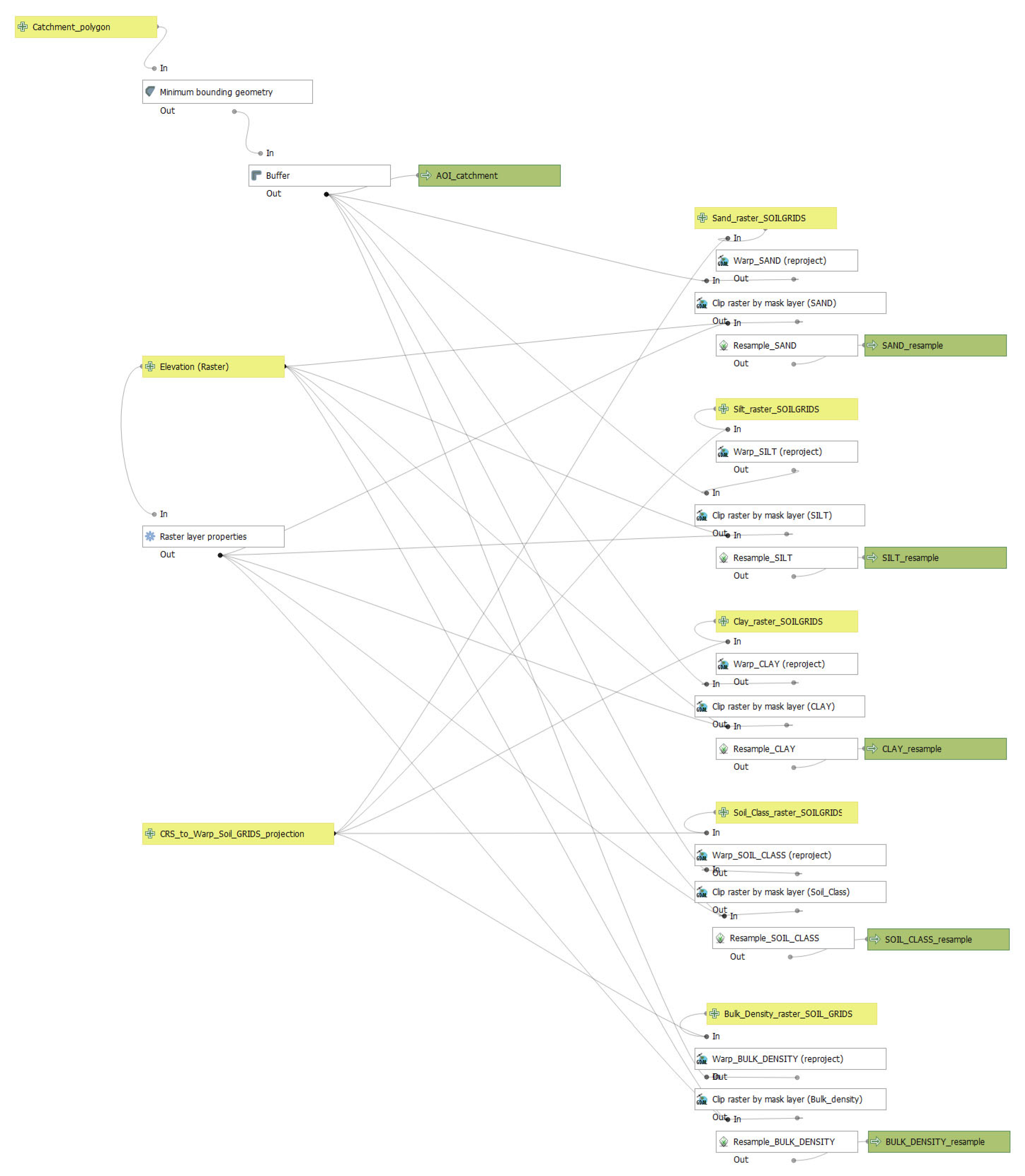
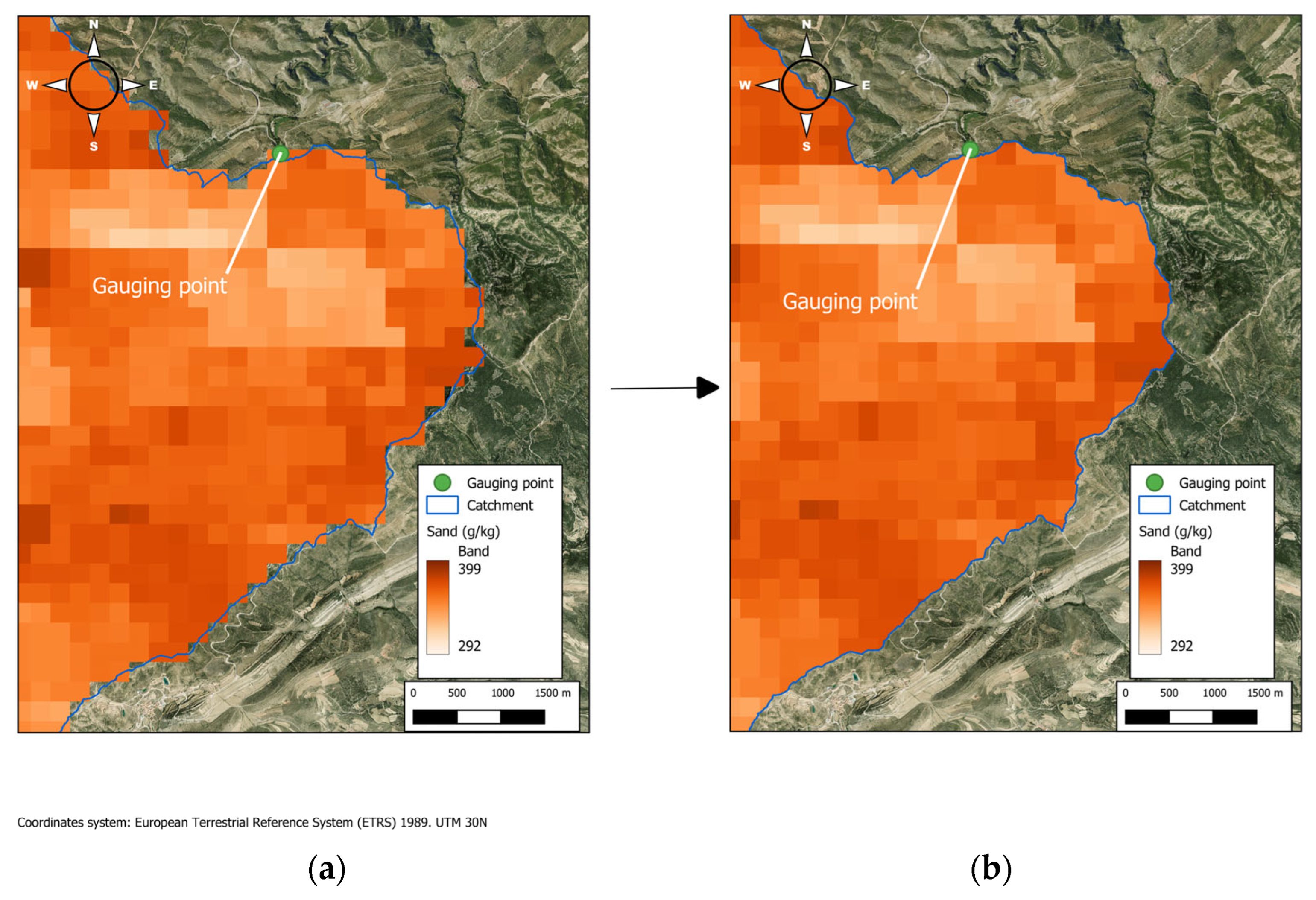
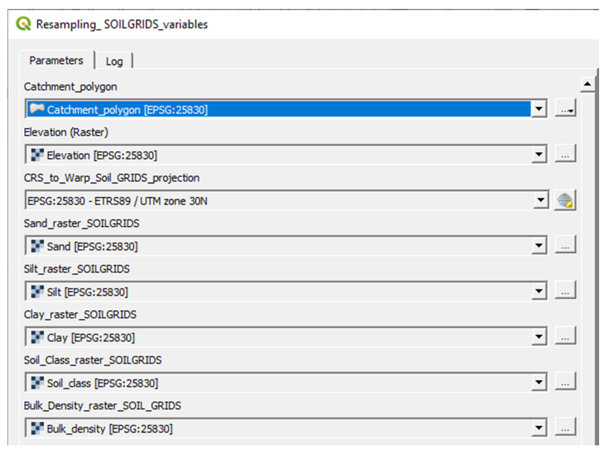
3.1.3. Spatial Homogenisation

Incorporating information related to soil physical properties required aligning the 25 ∗ 25 m pixels-size layers with 2 ∗ 2 m pixels layers containing topography and land use data.

We obtained the soil properties layers (soil textures, soil class and bulk density) from SoilGrids [39] in the form of 25 ∗ 25 m raster data. To ensure spatial consistency and maximise accuracy, we chose to downscale the SoilGrids pixel size rather than resampling the land use and topographical information to 25 ∗ 25 m. However, this gain in accuracy came at the expense of increased computational requirements. An overview of the resampling process is shown in Figure 11, while both the original and resampled images are presented in Figure 12.

We used the r.resample tool from GRASS toolbox to set the pixel size and the CRS parameter and provide both the vector catchment polygon and the DEM (see Figure 13). We did not face relevant issues during this process using the GRASS tools.

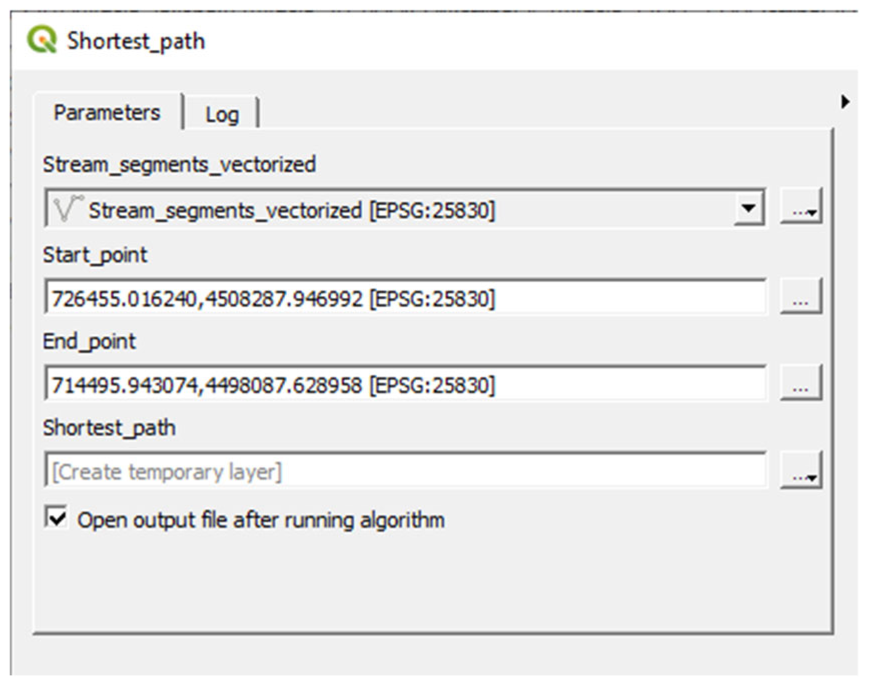
3.1.4. Flow Pathways

Identifying the flow paths through which water discharges across the catchment is essential for accurately modelling event-based hydrological processes and for parameterising distributed models.

We combined the shortest_path (point to point) algorithm, fed on the stream segments layers (delivered by the r.watershed tool), with the downstream and upstream endpoints. This routine was executed twice: first, from the highest point within the catchment to the downstream gauging point, and second, from the start of the main channel within the catchment to the same downstream gauging point. Although, in theory, both the downstream and upstream endpoints could be automatically defined, we consistently encountered challenges in automating the selection of the upstream point of the main channel, as identifying the initial point of the main drainage channel required expert judgment. Figure 14 and Figure 15 illustrate the parameter configuration and the resulting model outputs, respectively.

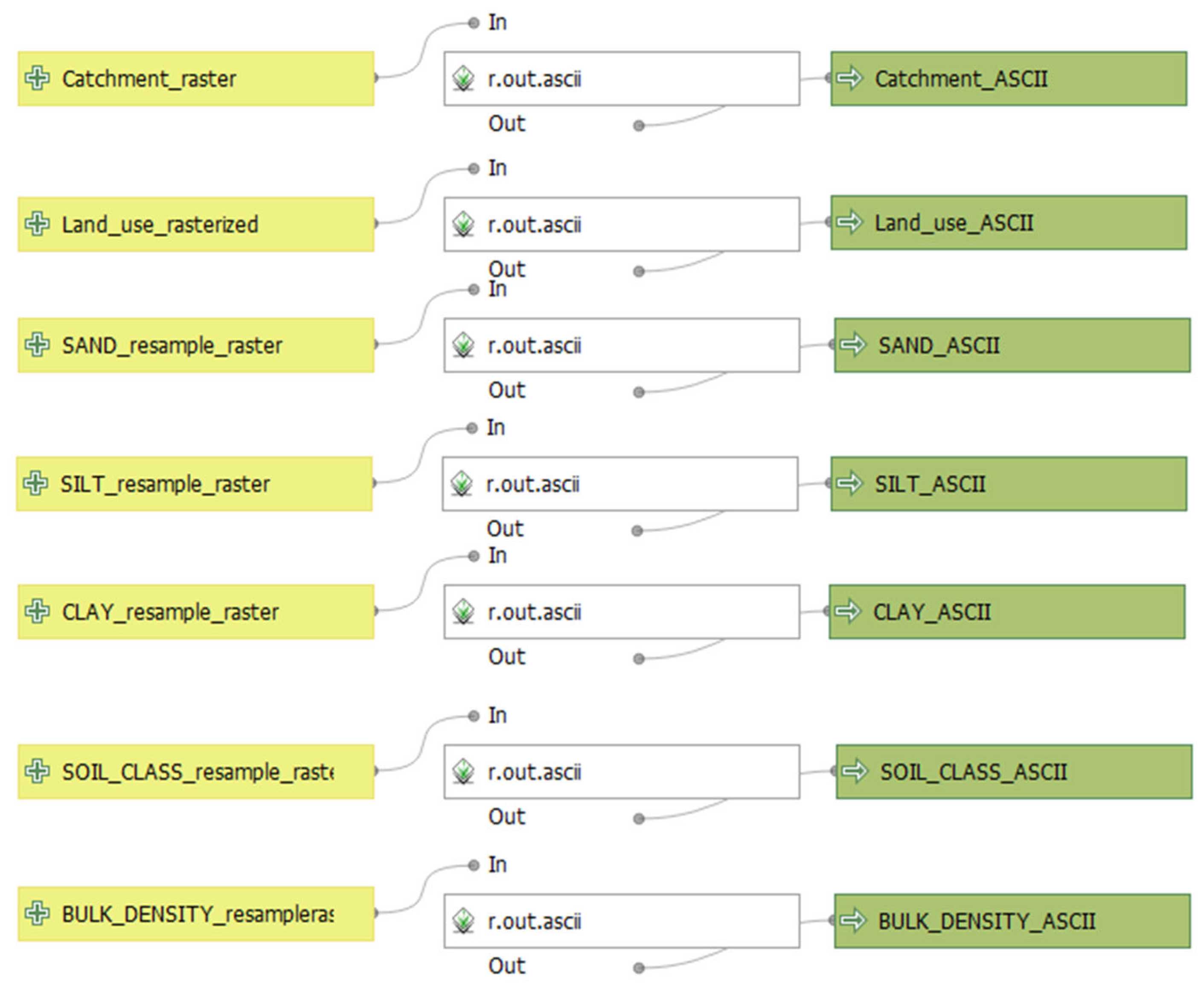
3.1.5. Catchment Characterisation and Exchangeable Files

Following these steps, we generated exchangeable information to support subsequent modelling workflows. We aimed at delivering both spatially distributed information (pixels’ land use, altimetry, bulk density, fractions of sand, silt, lime and soil class; see Figure 16) and summary metrics (discharging pathways length and slope, entire catchment area, land uses areas and aggregated areas of soil texture).

To process this information, we utilised zonal statistics tools for raster layers and generated a new field to use QGIS expressions in the Expression Builder to obtain the key attributes of vector layers. To ensure compatibility with programming environments, we exported the data in ASCII format, preserving the spatial structure as raster matrices (including basin, land use, sand, silt, clay, and bulk density rasters). Figure 17 presents the processing workflow architecture.

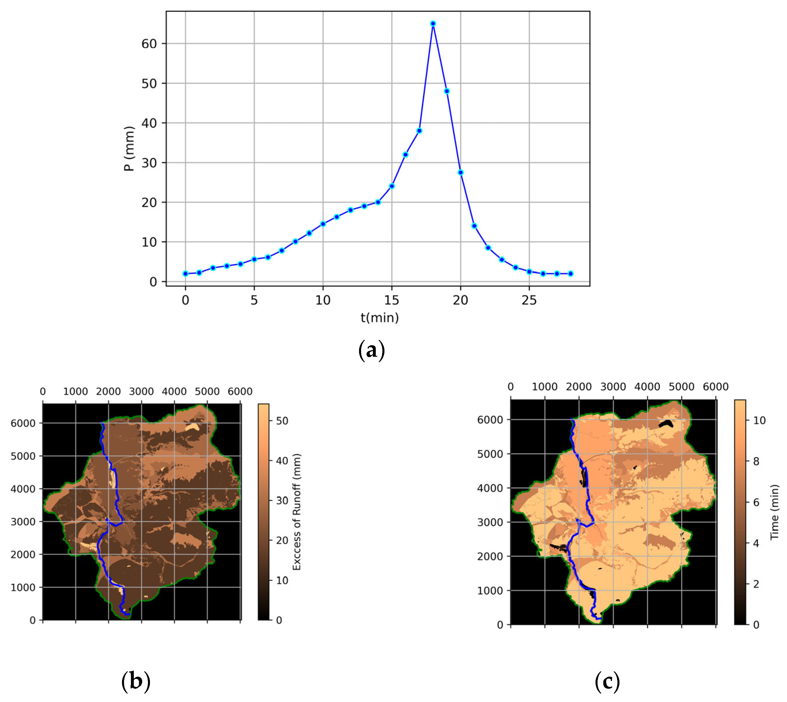
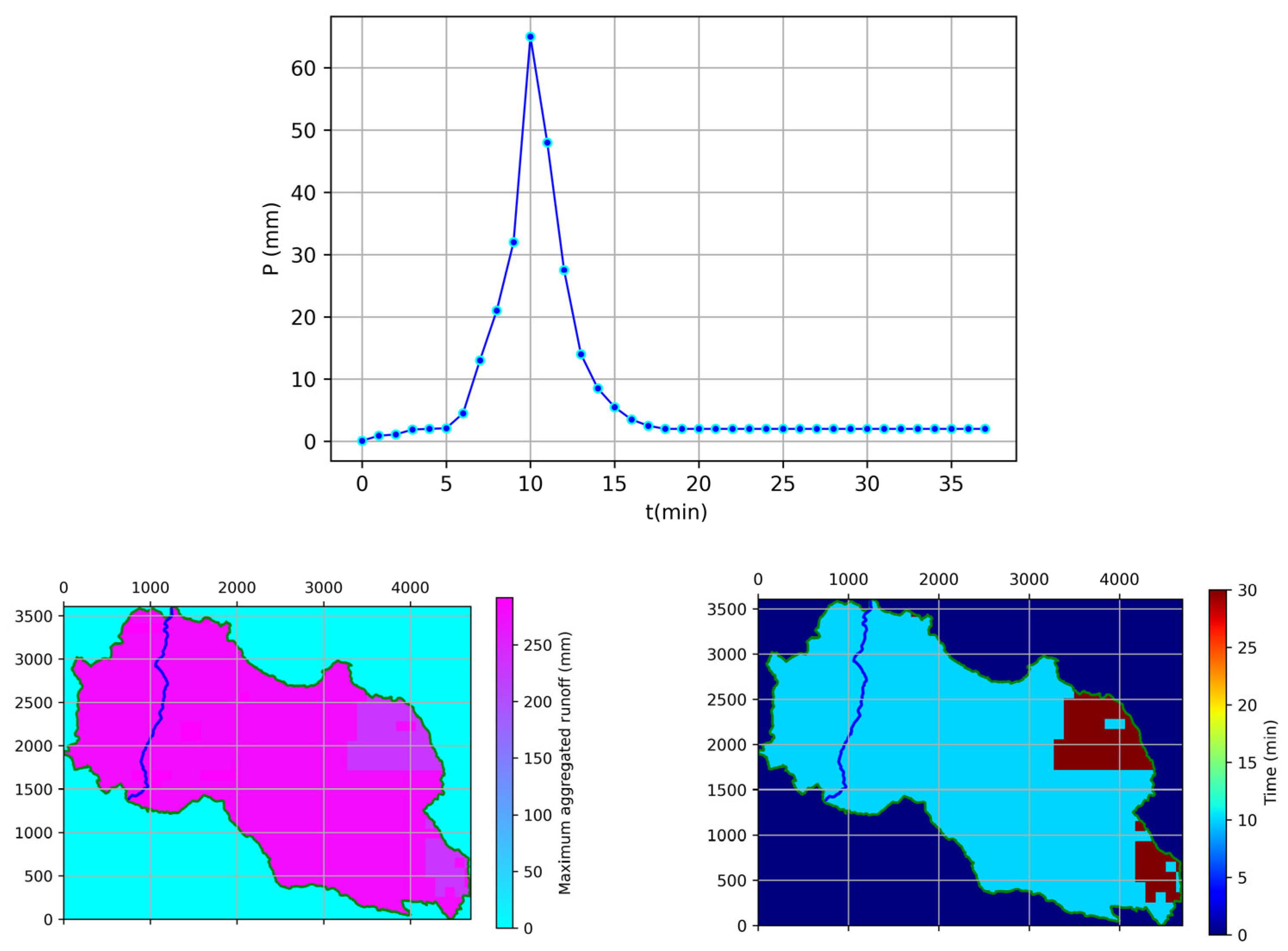
3.2. General Overview and Application Example

The previous processes can provide information for performing various advanced hydrological modelling tasks in different coding environments since the ASCII files can be readily accessed using various programming languages. As an example, we present, in this manuscript, cases studies using the QGIS outputs described in previous sections to implement the SCS curve number, the Green-Ampt model [36] and the Muskingum-Cunge routing method [37] within a Python environment.

Starting with the SCS curve number, we aimed to assign a curve number to each pixel to derive either an average catchment curve number for lumped modelling or a pixel-specific curve number analysis enabling distributed modelling. We illustrate this using the Aragón River upstream of the Canfranc gauging station (Huesca, Spain). Using the QGIS-derived ASCII land use data from SIOSE, we estimated the curve number and applied the SCS method to compute runoff excess on a per-pixel basis. Figure 17 shows the spatial distribution of the estimated runoff excess for a 60 mm storm event (producing the synthetic hyetograph presented in Figure 18) and the estimated time to runoff initiation for each 2 × 2 m pixel under a synthetic hyetograph, assuming runoff begins when rainfall exceeds the initial abstraction (Ia).

As shown in Figure 18 and Figure 19, we consider storm events with a volume of 60 mm falling over approximately 20 min. In the context of such storm events, evapotranspiration (approximately 10 mm/day in the most extreme areas and periods of the Ebro River basin) is negligible and can be excluded from the water balance.

Similarly, the soil property data from SoilGrids processed within QGIS enabled us to perform simulations based on the Green-Ampt infiltration equation. As a case study, we examined the Urenderro River upstream of the Barindano gauging station (Navarra, Spain). Using the ASCII files containing sand, silt, and clay fractions, we estimated soil textural classes using pedotransfer functions, assigning the Green-Ampt parameters to each pixel. These parameters were retrieved from Carsel and Parrish [40] and aided by Mualem [41] and van Genutchen [42] models for the conductivity and water retention curves. Figure 19 displays the maximum aggregated runoff, the time taken for the presented hyetograph to produce runoff and the maximum instantaneous runoff along with its timing.

For the kinematic wave model, we simulated the routing of a synthetic hydrograph along the Bailín River from the upstream cross-section to the Sabiñánigo gauging station (Huesca, Spain). We processed the QGIS ASCII to obtain the main channel location (Figure 20; 0–1 values), the channel topographical height (Figure 21; 0–z values) and main channel width (0–b values) with 2 ∗ 2 spatial resolution. The longitudinal slope was computed from topographical heights, supposing a straight triangular distance between both consecutive sections while Manning’s roughness coefficient and the cross-sections’ side slope were estimated from field observations.

Figure 22 presents the evolution of the hydrograph for a set of 39 selected cross sections. Figure 23 displays the spatial representation of the maximum flow and the maximum water depth derived from the kinematic wave hydrological simulation over a one pixel scale (the represented information refers to each 2 × 2 m pixels with each pixel representing each cross-section located at a 2.8 m distance from the previous one), and Figure 24 is the spatial representation of some hydrological variables.

3.3. Discussion

The integration of QGIS with Python routines for simulating event-based hydrological processes offers a flexible open-source framework for catchment-scale analyses. The proposed methodology demonstrates that producing GIS-based information to be processed in Python can improve the performance of events-based hydrological analysis in that environment. The main assumption underlying our approach is that spatial information can be used directly to parameterise hydrological models.

The proposed framework can improve the model parametrisation by for example leveraging the delineation of catchments and retrieving land uses or soil physical properties to be directly processed in Python. By taking advantage of QGIS’s graphical interface and geoprocessing tools, users can efficiently manage spatial datasets, while Python scripts enable automated parameter calculation, event-based simulation and results post-processing within the same environment. However, due to this integration, the proposed methodology is highly sensitive to the availability, accuracy and spatial resolution of the input data which can limit the performance of the hydrological model outputs. Since the QGIS outputs from processing spatial information are used to parametrise hydrological models, the greater the accuracy and quality of the spatial information, the higher the potential for improved model outputs. This is the main source of the uncertainty of the methodological process.

The methodological framework we present in this manuscript, unlike proprietary software packages such as ArcHydro [43], HEC-GeoHMS [44] or semi-proprietary frameworks like MIKE SHE [45], allows for a better control over the hydrological modelling chain, from spatial data pre-processing to computation and visualisation.

While other hydrological models do not allow for spatially distributed parametrisation, this proposal has the potential to improve model parameterisation, as it is directly linked to the resolution of the spatial data, which can enhance the performance of (semi-)distributed models and increase the accuracy of the representative values in lumped models. Conversely, this also implies that unrepresentative or erroneous spatial information will lead to poor parameterisation.

As mentioned previously, we have presented a set of common routines for producing data that can be easily managed in Python and used for the specific models presented here, as well as for many other models. For example, the time of concentration models presented in [46,47,48,49] can be easily computed within the Python environment using the GIS outputs we have provided. Similarly, the infiltration models of Philip [50] and Horton [51] can be parameterised using the outputs presented in this manuscript, following the approaches in [52,53,54]. Paying particular attention to the specific hydrological models used in this manuscript, it should be noted that we have not carried out specific validations for the examples presented; therefore, the outcomes cannot be compared with actual observations. Specific model calibration or validation based on the proposed framework could be performed in future work, for example, to analyse the accuracy of parameter estimates. Similarly, given the short duration of the storm events considered (see Figure 17 and Figure 18), we have neglected the effect of evapotranspiration incorporated in the theoretical definition of the water balance presented in Equations (2) and (3). Future studies using the proposed methodology could extend the duration of the analysed events and incorporate the effect of evapotranspiration in the water balance.

During the application of this workflow, we identified certain limitations, particularly convergence issues in some QGIS tools when processing highly complex geometries. Despite these limitations, we present a general framework for producing exchangeable spatial information that can be easily processed in Python. While this paper details the use of the framework for specific hydrological methods, the overall approach—and, in many cases, the information used and the outputs presented in this paper—can be applied to a wide range of hydrological simulations.

Exiting proprietary GIS-integrated hydrological models typically provide user-friendly interfaces and robust toolsets for delineating watersheds, extracting drainage networks, and parameterising hydrological models. However, they often operate as black boxes, limiting the user’s ability to customise routines. In contrast, the QGIS−Python approach leverages QGIS’s extensive GIS capabilities while allowing users to implement and modify Python scripts for parameter estimation, rainfall-runoff modelling and post-processing of results, promoting transparency and adaptability in the modelling workflow. Practitioners can leverage the presented framework for practical hydrological studies by coding their specific functions depending on the analysis they wish to perform. This can help them develop modelling tools specifically tailored to address questions not covered by proprietary models.

Future work could focus on integrating additional Python libraries for hydrological modelling (e.g., PyCatch, PyTOPKAPI), coupling with hydraulic models for floodplain analysis, and developing user-friendly interfaces within QGIS to facilitate the adoption of the methodology by practitioners and stakeholders without extensive programming experience. However, despite the potential development of user-friendly interfaces, we strongly believe that leveraging Python IDEs to develop tailored applications remains the best alternative for maximising the utility of the presented methods.

Similarly, future developments could target the integration of weather information from weather stations by leveraging spatial interpolation tools (i.e., Krigging algorithms) to provide spatially distributed information for hydrological models. Of particular interest for addressing events-based hydrological processes would be to develop of tools capable of processing weather station data to extract storm events and subsequently apply spatial interpolation to generate distributed storm event datasets for hydrological modelling.

4. Conclusions

In this manuscript, we have presented a set of QGIS-based tools for processing geographical information and producing outputs tailored for running hydrological models. The outputs are perfectly suited for developing tools in any common programming language since they are provided in plain text.

The methods presented are based on easily available information from satellite imagery so they can be performed with no relevant limitations. The integration between QGIS outputs and hydrological modelling in common programming languages provides particular versatility. The methodological framework we provide opens up opportunities to perform tailored modelling tools which represents a step forward in comparison to existing encapsulated analysis packages. Both the ability of QGIS to process spatial information and the ability of Python to develop enhanced calculation routines are boosted with the proposed method, which will maximise the performance of the hydrological analysis carried out.

It is important to note that the hydrological model simulations included in this study are intended solely to demonstrate the applicability of the proposed GIS−Python framework for spatial data processing and hydrological model input. Calibration and validation of these models were not performed, which is beyond the scope of this methodological contribution.

Future developments should be aimed at providing automatic tools for performing the tasks performed manually, developing self-checking routines for avoiding common errors in processing the information. While the absence of user-friendly interfaces in Python programming can prevent the extensive spread of the method, some tuned GUIs could be developed for addressing some specific tasks. However, the programming operation should be addressed in a pure coding environment to avoid limiting the efficacy of the proposed framework.

References

1. Herrera, P.A.; Marazuela, M.A.; Hofmann, T. Parameter estimation and uncertainty analysis in hydrological modeling. Wiley Interdiscip. Rev. Water 2022, 9, e1569. [Google Scholar] [CrossRef]
2. Liu, Y.; Gupta, H.V. Uncertainty in hydrologic modeling: Toward an integrated data assimilation framework. Water Resour. Res. 2007, 43, 1–18. [Google Scholar] [CrossRef]
3. Oreskes, N.; Shrader-Frechette, K.; Belitz, K. Verification, Validation, and Confirmation of Numerical Models in the Earth Sciences. Science 1979, 263, 641–646. [Google Scholar] [CrossRef] [PubMed]
4. Hrozencik, R.A.; Manning, D.T.; Suter, J.F.; Goemans, C.; Bailey, R.T. The Heterogeneous Impacts of Groundwater Management Policies in the Republican River Basin of Colorado. Water Resour. Res. 2017, 53, 10757–10778. [Google Scholar] [CrossRef]
5. Salvadore, E.; Bronders, J.; Batelaan, O. Hydrological modelling of urbanized catchments: A review and future directions. J. Hydrol. 2015, 529, 62–81. [Google Scholar] [CrossRef]
6. Wada, Y.; Bierkens, M.F.P.; de Roo, A.; Dirmeyer, P.A.; Famiglietti, J.S.; Hanasaki, N.; Konar, M.; Liu, J.; Müller Schmied, H.; Oki, T.; et al. Human-water interface in hydrological modelling: Current status and future directions. Hydrol. Earth Syst. Sci. 2017, 21, 4169–4193. [Google Scholar] [CrossRef]
7. Chang, F.-J.; Wang, Y.-C.; Tsai, W.P. Modelling Intelligent Water Resources Allocation for Multi-users. Water Resour. Manag. 2016, 30, 1395–1413. [Google Scholar] [CrossRef]
8. Letcher, R.A.; Croke, B.F.W.; Jakeman, A.J. Integrated assessment modelling for water resource allocation and management: A generalised conceptual framework. Environ. Model. Softw. 2007, 22, 733–742. [Google Scholar] [CrossRef]
9. Nousiainen, R.; Warsta, L.; Turunen, M.; Huitu, H.; Koivusalo, H.; Pesonen, L. Analyzing subsurface drain network performance in an agricultural monitoring site with a three-dimensional hydrological model. J. Hydrol. 2015, 529, 82–93. [Google Scholar] [CrossRef]
10. Ursulak, J.; Coulibaly, P. Integration of hydrological models with entropy and multi-objective optimization based methods for designing specific needs streamflow monitoring networks. J. Hydrol. 2021, 593, 125876. [Google Scholar] [CrossRef]
11. Hagemann, S.; Chen, C.; Clark, D.B.; Folwell, S.; Gosling, S.N.; Haddeland, I.; Hanasaki, N.; Heinke, J.; Ludwig, F.; Voss, F.; et al. Climate change impact on available water resources obtained using multiple global climate and hydrology models. Earth Syst. Dyn. 2013, 4, 129–144. [Google Scholar] [CrossRef]
12. Xu, C.Y. Modelling the effects of climate change on water resources in central Sweden. Water Res. Manag. 2000, 14, 177–189. [Google Scholar] [CrossRef]
13. Brocca, L.; Ciabatta, L.; Massari, C.; Moramarco, T.; Hahn, S.; Hasenauer, S.; Kidd, R.; Dorigo, W.; Wagner, W.; Levizzani, V. Soil as a natural rain gauge: Estimating global rainfall from satellite soil moisture data. J. Geophys. Res. Atmos. 2014, 119, 5128–5141. [Google Scholar] [CrossRef]
14. Massari, C.; Crow, W.; Brocca, L. An assessment of the accuracy of global rainfall estimates without groundbased observations. Hydrol. Earth Syst. Sci. 2017, 21, 4347–4361. [Google Scholar] [CrossRef]
15. Manfreda, S.; Caylor, K.K.; Good, S.P. An ecohydrological framework to explain shifts in vegetation organization across climatological gradients. Ecohydrology 2017, 10, e1809. [Google Scholar] [CrossRef]
16. Zhu, L.; Wang, H.; Tong, C.; Liu, W.; Du, B.T. Evaluation of ESA Active, Passive and Combined Soil Moisture Products Using Upscaled Ground Measurements. Sensors 2019, 19, 2718. [Google Scholar] [CrossRef] [PubMed]
17. Meng, X.; Mao, K.; Meng, F.; Shen, X.; Xu, T.; Cao, M. Long-Term Spatiotemporal Variations in Soil Moisture in North East China Based on 1-km Resolution Downscaled PassiveMicrowave Soil Moisture Products. Sensors 2019, 19, 3527. [Google Scholar] [CrossRef] [PubMed]
18. Glenn, E.P.; Neale, C.M.U.; Hunsaker, D.J.; Nagler, P.L. Vegetation index-based crop coefficients to estimate evapotranspiration by remote sensing in agricultural and natural ecosystems. Hydrol. Process. 2011, 25, 4050–4062. [Google Scholar] [CrossRef]
19. Castellví, F.; Cammalleri, C.; Ciraolo, G.; Maltese, A.; Rossi, F. Daytime sensible heat flux estimation over heterogeneous surfaces using multitemporal land-surface temperature observations. Water Resour. Res. 2016, 52, 3457–3476. [Google Scholar] [CrossRef]
20. Bastiaanssen, W.G.M.; Menenti, M.; Feddes, R.A.; Holtslag, A.A.M. A remote sensing surface energy balance algorithm for land (SEBAL): 1. Formulation. J. Hydrol. 1998, 212–213, 198–212. [Google Scholar] [CrossRef]
21. Schumann, G.J.P.; Domeneghetti, A. Exploiting the proliferation of current and future satellite observations of rivers. Hydrol. Process. 2016, 30, 2891–2896. [Google Scholar]
22. Domeneghetti, A.; Castellarin, A.; Tarpanelli, A.; Moramarco, T. Investigating the uncertainty of satellite altimetry products for hydrodynamic modelling. Hydrol. Process. 2008, 29, 4908–4918. [Google Scholar] [CrossRef]
23. Schneider, R.; Godiksen, P.N.; Villadsen, H.; Madsen, H.; Bauer-Gottwein, P. Application of CryoSat-2 altimetry data for river analysis and modelling. Hydrol. Earth Syst. Sci. 2017, 21, 751–764. [Google Scholar] [CrossRef]
24. Tourian, M.J.; Tarpanelli, A.; Elmi, O.; Qin, T.; Brocca, L.; Moramarco, T.; Sneeuw, N. Spatiotemporal densification of river water level time series by multimission satellite altimetry. Water Resour. Res. 2016, 52, 1140–1159. [Google Scholar] [CrossRef]
25. Schumann, A.H.; Funke, R.; Schultz, G.A. Application of a geographic information system for conceptual rainfall–runoff modeling. J. Hydrol. 2000, 240, 45–61. [Google Scholar] [CrossRef]
26. Durand, M.; Andreadis, K.M.; Alsdorf, D.E.; Lettenmaier, D.P.; Moller, D.; Wilson, M. Estimation of bathymetric depth and slope from data assimilation of swath altimetry into a hydrodynamic model. Geophys. Res. Lett. 2008, 10, L20401. [Google Scholar] [CrossRef]
27. Schlosser, C.A.; Houser, P.R. Assessing a satellite-era perspective of the global water cycle. J. Clim. 2017, 20, 1316–1338. [Google Scholar] [CrossRef]
28. Levizzani, V.; Cattani, E. Satellite remote sensing of precipitation and the terrrestrial water cycle in a changing climate. Remote Sens. 2019, 11, 2301. [Google Scholar] [CrossRef]
29. Kidd, C.; Huffman, G.; Maggioni, V.; Chambon, P.; Oki, R. The global satellite precipitation constellation: Current status and future requirement. Bull. Amer. Meteorol. Soc. 2021, 102, E1844–E1861. [Google Scholar] [CrossRef]
30. Fang, J.; Yang, W.; Luan, Y.; Du, J.; Lin, A.; Zhao, L. Evaluation of the TRMM 3B42 and GPMIMERG products for extreme precipitation analysis over China. Atmos. Res. 2019, 223, 24–38. [Google Scholar] [CrossRef]
31. Prakash, S.; Mitra, A.K.; Pai, D.S.; AghaKouchak, A. From TRMM to GPM: How well can heavy rainfall be detected from space? Adv. Water Resour. 2016, 88, 1–7. [Google Scholar] [CrossRef]
32. Chen, H.; Yong, B.; Shen, Y.; Liu, J.; Hong, Y.; Zhang, J. Comparison analysis of six purely satellite-derived global precipitation estimates. J. Hydrol. 2020, 581, 124376. [Google Scholar] [CrossRef]
33. Bogena, H.R.; Huisman, J.A.; Güntner, A.; Hübner, C.; Kusche, J.; Jonard, F.; Vey, S.; Vereecken, H. Emerging methods for noninvasive sensing of soil moisture dynamics from field to catchment scale: A review. WIREs Water 2015, 2, 635–647. [Google Scholar] [CrossRef]
34. Jain, M.K.; Kothyari, U.C.; Raju, K.G.R. A GIS based distributed rainfall–runoff model. J. Hydrol. 2004, 299, 107–135. [Google Scholar] [CrossRef]
35. Zollweg, J.A.; Gburek, W.J.; Steenhuis, T.S. SMoRMod—A GIS-integrated rainfall-runoff model. Trans. ASAE 1996, 39, 1299–1307. [Google Scholar] [CrossRef]
36. Green, W.H.; Ampt, G.A. Studies on soil physics. J. Agric. Sci. 1911, 4, 1–24. [Google Scholar] [CrossRef]
37. Cunge, J.A. On the subject of a flood propagation computation method (Muskingum method). J. Hydraul. Res. 1969, 7, 205–230. [Google Scholar] [CrossRef]
38. Chow, V.T.; Maidment, D.R.; Mays, L. Applied Hydrology; McGrawHill: New York, NY, USA, 1988. [Google Scholar]
39. Hengl, T.; De Jesus, J.M.; Heuvelink, G.B.M.; Gonzalez, M.R.; Kilibarda, M.; Blagotić, A.; Shangguan, W.; Wright, M.N.; Geng, X.; Bauer-Marschallinger, B.; et al. SoilGrids250m: Global gridded soil information based on machine learning. PLoS ONE 2017, 12, e0169748. [Google Scholar] [CrossRef]
40. Carsel, R.F.; Parrish, R.S. Developing joint probability distributions of soil water retention characteristics. Water Resour. Res. 1988, 24, 755–769. [Google Scholar] [CrossRef]
41. Mualem, Y. Hydraulic conductivity of unsaturated soils: Prediction and formulas. Methods Soil Anal. Part 1 Phys. Mineral. Methods 1986, 5, 799–823. [Google Scholar]
42. Van Genuchten, M.T. A closed-form equation for predicting the hydraulic conductivity of unsaturated soils. Soil Sci. Soc. Am. J. 1980, 44, 892–898. [Google Scholar] [CrossRef]
43. Maidment, D.R. ArcHydro: GIS for Water Resources; ESRI Press: Redlands, CA, USA, 2002. [Google Scholar]
44. USACE. HEC-GeoHMS User’s Manual, Version 4.2; U.S. Army Corps of Engineers; Hydrologic Engineering Center: Davis, CA, USA, 2009.
45. Abbott, M.B.; Bathurst, J.C.; Cunge, J.A.; O’Connell, P.E.; Rasmussen, J. An introduction to the European Hydrological System—Systeme Hydrologique Europeen, “SHE”, 1: History and philosophy of a physically-based, distributed modelling system. J. Hydrol. 1986, 87, 45–59. [Google Scholar] [CrossRef]
46. Kirpich, Z.P. Time of concentration of small agricultural watersheds. Civ. Civil. Eng. 1940, 10, 362. [Google Scholar]
47. NRCS (National Research Conservation Service). Ponds—Planning, Design, Construction; Agriculture Handbook no 590; US Natural Resources Conservation Service: Washington DC, USA, 1997.
48. Giandotti, M. Previsione Delle Piene e Delle Magre dei Corsid’acqua; Istituto Poligrafico dello Stato: Rome, Italy, 1934; Volume 8, pp. 107–117.
49. Johnstone, D.; Cross, W.P. Elements of Applied Hydrology; Ronald Press: New York, NY, USA, 1949. [Google Scholar]
50. Philip, J.R. Theory of infiltration. Adv. Hydrosci. 1969, 5, 215–305. [Google Scholar]
51. Horton, R.E. An approach toward physical interpretation of infiltration capacity. Soil Sci. Soc. Am. Proc. 1940, 5, 399–417. [Google Scholar] [CrossRef]
52. Ross, P.J.; Haverkamp, R.; Parlange, J.Y. Calculating parameters for infiltration equations from soil hydraulic functions. Transp. Porous Media 1996, 24, 315–339. [Google Scholar] [CrossRef]
53. Brutsaert, W. Vertical infiltration in dry soil. Water Resour. Res. 1977, 13, 363–368. [Google Scholar] [CrossRef]
54. Smith, R.E.; Parlange, J.Y. A parameter-efficient hydrologic infiltration model. Water Resour. Res. 1978, 14, 533–538. [Google Scholar] [CrossRef]
Figure 1. Graphical representation of the data collection process and sources.
Water 17 02160 g001
Figure 2. Idealised catchment (a) and processes’ workflow (b) for the hydrological simulations.
Water 17 02160 g002
Figure 3. Area of study representing the selected catchments in the Ebro River basin (images retrieved from the Spanish national mapping provider, Instituto Geográfico Nacional at https://centrodedescargas.cnig.es/CentroDescargas/index.jsp#, accessed on 16 May 2025).
Water 17 02160 g003
Figure 4. QGIS model 1. Catchment delimitation (representing yellow boxes represent the model inputs, white boxes indicate the functions utilised to process these inputs, and green boxes show the model outputs). The screenshot was obtained from the QGIS software (QGIS Development Team, 2024).
Water 17 02160 g004
Figure 5. Setup for r.watershed and r.water.outlet algorithms. The screenshot was obtained from the QGIS software (QGIS Development Team, 2024).
Water 17 02160 g005
Figure 6. GRASS r.water tool outputs (images retrieved from the Spanish national mapping provider, Instituto Geográfico Nacional at https://centrodedescargas.cnig.es/CentroDescargas/index.jsp#, accessed on 10 July 2025).
Water 17 02160 g006
Figure 7. Detail of the downstream end point selection for delineating the catchment (images retrieved from the Spanish national mapping provider, Instituto Geográfico Nacional at https://centrodedescargas.cnig.es/CentroDescargas/index.jsp# accessed on 10 July 2025).
Water 17 02160 g007
Figure 8. QGIS model 2: topographical factors and land use. The screenshot was obtained from the QGIS software (QGIS Development Team, 2024).
Water 17 02160 g008
Figure 9. Parameters’ tuning for models clip and rasterise tools. The screenshot was obtained from the QGIS software (QGIS Development Team, 2024).
Water 17 02160 g009
Figure 10. Catchment bounded topography and land uses (images and digital elevation model retrieved from the Spanish national mapping provider, Instituto Geográfico Nacional at https://centrodedescargas.cnig.es/CentroDescargas/index.jsp#, accessed on 10 July 2025, and land use data from the Spanish Land Use System (SIOSE)—Instituto Geográfico Nacional, 2016).
Water 17 02160 g010
Figure 11. QGIS model 3: soil variables resampling. The screenshot was obtained from the QGIS software (QGIS Development Team, 2024).
Water 17 02160 g011
Figure 12. Original and resampled images, showing the differences in the pixel size between the two: (a) the original one; and (b) the resampled one (images retrieved from the Spanish national mapping provider, Instituto Geográfico Nacional at https://centrodedescargas.cnig.es/CentroDescargas/index.jsp#, accessed on 10 July 2025).
Water 17 02160 g012
Figure 13. Setting up of the r.resample tool. The screenshot was obtained from the QGIS software (QGIS Development Team, 2024).
Water 17 02160 g013
Figure 14. Setting up of the shortest_path tool. The screenshot was obtained from the QGIS software.
Water 17 02160 g014
Figure 15. The shortest path model’s outcome (images retrieved from the Spanish national mapping provider, Instituto Geográfico Nacional at https://centrodedescargas.cnig.es/CentroDescargas/index.jsp#, accessed on 10 July 2025).
Water 17 02160 g015
Figure 16. Summary of spatially distributed information comprising the DEM (a), the bulk density (b), the clay (c), sand (d) and silt (e) soil fractions and as a result of those the soil (textural) classes (f) and finally the land uses (g).
Water 17 02160 g016
Figure 17. Transformation to ASCII format. The screenshot was obtained from the QGIS software.
Water 17 02160 g017
Figure 18. (a) Synthetic hyetograph of a 60 mm storm event; (b) spatial distribution of excess runoff as estimated by the curve number method from a 60 mm storm event; (c) time taken for the synthetic hyetograph to produce runoff.
Water 17 02160 g018
Figure 19. Simulated hyetograph, maximum aggregated runoff, time taken to produce runoff, maximum instant runoff and time at which it was observed.
Water 17 02160 g019
Figure 20. Catchment limits and main channel location.
Water 17 02160 g020
Figure 21. Channel heights from GIS files and computed longitudinal slope.
Water 17 02160 g021
Figure 22. Evolution of the synthetic hydrograph across a set of 39 cross-sections.
Water 17 02160 g022
Figure 23. Profile of the peak flow, maximum velocity, maximum water depth and Froude number across the cross-sections.
Water 17 02160 g023
Figure 24. Spatial representation of the peak flow, maximum velocity, maximum water depth and Froude number across the cross-sections.
Water 17 02160 g024aWater 17 02160 g024b