Hydraulic Modeling of Newtonian and Non-Newtonian Debris Flows in Alluvial Fans: A Case Study in the Peruvian Andes

Abstract

Non-Newtonian debris flows represent a critical challenge for hydraulic infrastructure in mountainous regions, often causing significant damage and service disruption. However, current models typically simplify these flows as Newtonian, leading to inaccurate design assumptions. This study addresses this gap by comparing the hydraulic behavior of Newtonian and non-Newtonian flows in an alluvial fan, using the Amoray Gully in Apurímac, Peru, as a case study. This gully intersects the Interoceánica Sur national highway via a low-water crossing (baden), making it a relevant site for evaluating debris flow impacts on critical road infrastructure. The methodology integrates hydrological analysis, rheological characterization, and hydraulic modeling. QGIS 3.16 was used for watershed delineation and extraction of physiographic parameters, while a high-resolution topographic survey was conducted using an RTK drone. Rainfall-runoff modeling was performed in HEC-HMS 4.7 using 25 years of precipitation data, and hydraulic simulations were executed in HEC-RAS 6.6, incorporating rheological parameters and calibrated with the footprint of a historical event (5-year return period). Results show that traditional Newtonian models underestimate flow depth by 17% and overestimate velocity by 54%, primarily due to unaccounted particle-collision effects. Based on these findings, a multi-barrel circular culvert was designed to improve debris flow management. This study provides a replicable modeling framework for debris-prone watersheds and contributes to improving design standards in complex terrain. The proposed methodology and findings offer practical guidance for hydraulic design in mountainous terrain affected by debris flows, especially where infrastructure intersects active alluvial fans.

1. Introduction

Globally, since the 1980s, there has been a significant surge in research on vulnerability to natural disasters, driven by the growing impacts of climate change. Among these, floods and their effects on transportation infrastructure have garnered particular attention, prompting advancements in resilience engineering [1]. Resilience emphasizes effective floodwater management, which mitigates risks to both populations and infrastructure [2]. As climate change has amplified the intensity and frequency of flooding in recent decades [3], enhancing infrastructure resilience has become a critical priority especially for vital systems like transportation networks, which must remain safe and fully operational [4]. Flood risk analysis through hydrological modeling and forecasting is critical for assessing flood resilience, as water depth and spatial extent directly determine transportation infrastructure vulnerability [1]. To improve accuracy, hydraulic simulation tools such as 1D HEC-RAS [5], 2D Iber [6,7], and HEC-RAS 2D [8], integrated with software like GIS and HEC-HMS, are essential for developing flood risk reduction strategies [9]. These tools have been extensively applied to critical transportation infrastructure, particularly railway networks [10] and bridges [11,12,13]. However, significant research gaps remain in modeling debris flow interactions with transportation networks, especially highways traversing alluvial fans where non-Newtonian flows dominate. This research gap is particularly critical in regions like Peru, where such events frequently disrupt vital transport corridors.

Peru is one of the most vulnerable countries to climate change alterations, which produces several natural phenomena, such as floods, that intensify their consequences [14]. In the 1997–1998 ENSO (El Niño-Southern Oscillation) event, Peru and Ecuador were the most affected countries in South America due to widespread flooding and landslides [15]. That situation gave the authorities an opportunity to build appropriate infrastructure and develop adequate prevention plans for subsequent natural disasters. Nonetheless, years later, during the 2016–2017 ENSO event—when the Rimac river basin experienced an extreme increase of more than 5000% in precipitation compared to normal levels [16]—the nation’s infrastructure vulnerability was exposed [17]: 10,251 km of roads were affected, 4030 km were destroyed, and for rural roads, 5939 km were affected, and 2398 km were destroyed [18]. Also, in 2023, heavy rain resulted in 638.3 km of roads being affected and 59.3 km of roads being destroyed; 68.5 km of rural roads were affected, and 8.6 km were destroyed [19]. Such a concerning situation reflects the lack of preparedness of the country to hydrological phenomena, highlighting the value of this research and, as Espinoza Vigil et al. [17] stated, the need for more representative models of disaster events to mitigate associated risks.

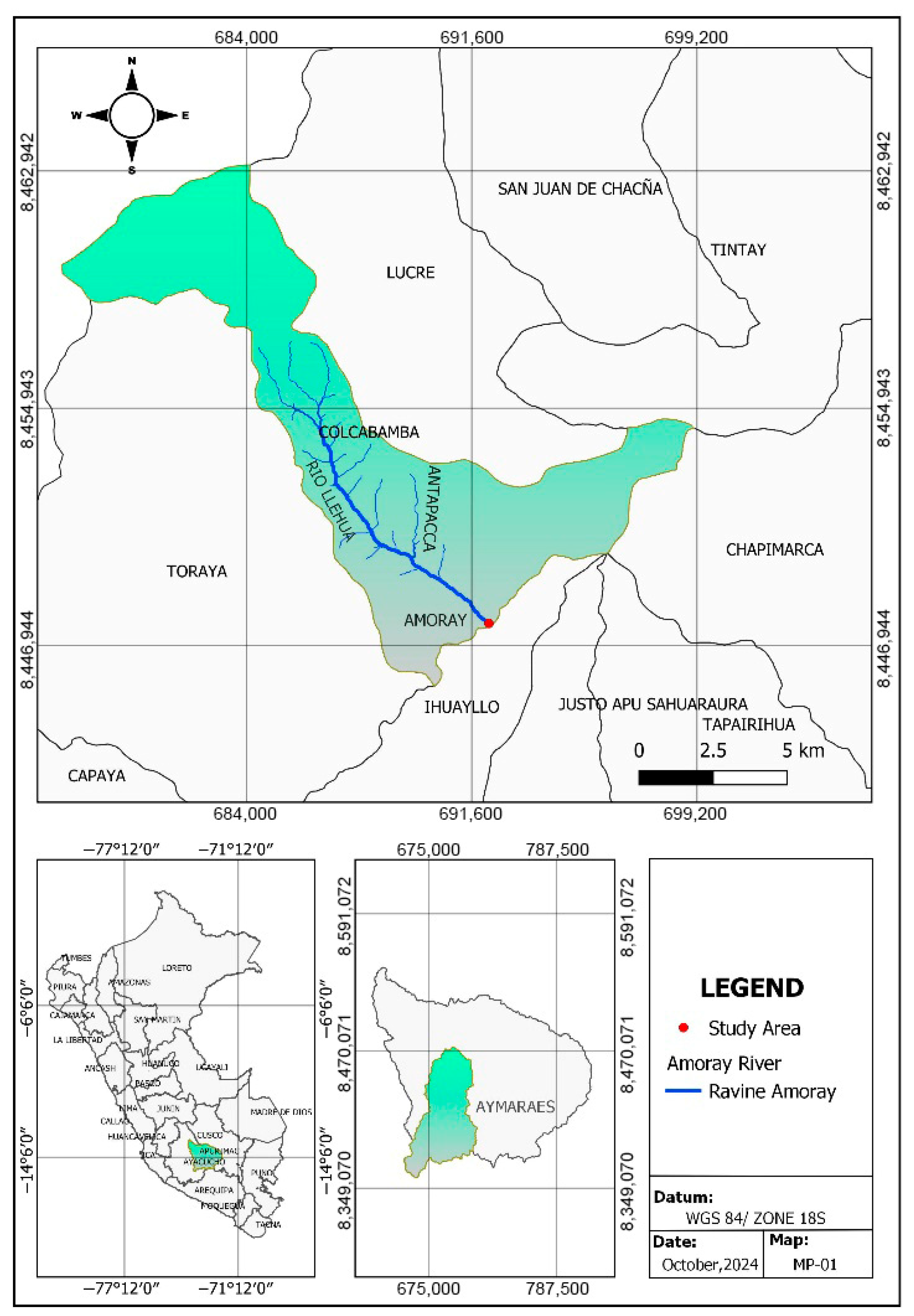
In recent years, Apurímac, Peru, has been one of the cities that has suffered the greatest damage due to the ENSO phenomenon. From January to March of 2024, interruptions were observed on the Interoceánica Sur national highway due to heavy rains, triggering mass movements downstream, causing damage to hydraulic structures, agricultural areas, and severing national transport corridors. As a result, in January of 2024, the Peruvian government declared a State of Emergency in Apurimac due to the impact of the heavy rains [20]. This case demonstrates how traditional clear water models fail to capture debris flow dynamics, highlighting the necessity of non-Newtonian modeling. It also renders the infrastructure unsustainable, as achieving sustainability goals largely depends on the planning stage [21].

Regarding non-Newtonian flow modeling, a literature review was performed, and the following research was found (

Table 1. Literature review on non-Newtonian flow modeling.

Author	Year	Relevance	Software	Natural Hazard	Case Study
Paricio et al. [22]	2019	The development of numerous flood events with rheological properties is detailed.	FLO-2D	Hurricane and tropical storm in a watershed.	Basin Tzununá, Lake Atlitán in Guatemala.
Laura et al. [23]	2019	This study outlines the simulation criteria for mud and debris flows to assess the hazard level in vulnerable areas.	FLO-2D	Debris flows in the Karla mine.	Lluta Gully in Tacna, Perú.
Almeida et al. [24]	2019	Numerical modeling and simulation techniques are presented to reproduce the transport and deposition processes of the debris flow.	FLO-2D	Debris flows in a watershed where a community is situated.	Mirave in Locumba, Perú.
Shengshan et al. [25]	2021	Evaluation of danger of debris slides in small watersheds.	FLO-2D	Debris flows in gullies.	Eryang River watershed in Gansu, China.
Martinez [26]	2022	The comparison and limitation of the HEC-RAS and FLO-2D software is determined based on two events.	QGIS, FLO-2D, and HEC-RAS 6.1.	Debris flows in gullies.	Acerillas and La Mesill gullies, Huasco river basin in Chile.
Bonasia et al. [27]	2022	The numerical modeling of erosive phenomena of volcanic deposits, as well as of flooding in the volcanic area are presented.	Iber 3.2.0.	Erosion and floods in the volcanic environment of an island’s northern region, where the main village is located.	Island of Vulcano, Aeolian Archipelago in Italy.
Gibson et al. [28]	2022	The prototype-scale verification and validation of the HEC-RAS model methods are presented.	HEC-RAS 6.1 2D.	Flood following a forest fire in a watershed and tailings dam breach.	Santa Bárbara in California. EEUU and Brumadinho, Minas Gerais in Brasil.
Alamanos et al. [8]	2023	A novel approach to the representation of flooding after a fire is presented.	WRF-ARW v4.2, Q-GIS, and HEC-RAS 2D.	Post-fire flash-flood event.	The Kineta cathment in Central Greece.
Ortiz-Giraldo et al. [6]	2023	A methodology for estimating stream clogging by rainfall-induced shallow landslides is presented.	SLIDE, RAMMS-DF, HEC-HMS, and IBER 2D.	Obstruction of water streams generated by shallow landslides.	Subbasin in the Ovejas river, Colombia.
Masoumi et al. [29]	2024	The study investigates peak flow in urban rivers, accounting for the impacts of climate change, debris flow contributing to flood risk, and the influence of woody debris.	HEC-RAS 2D.	Climate change and debris flow in urban rivers.	Farahzad River basin in Tehran, Iran.
Zahroni et al. [30]	2024	Rain-induced debris flow in a volcanic eruption zone is investigated by analyzing the curve number.	HEC-HMS 4.10. and HEC-RAS 6.3.1. 2D.	Debris flow post volcanic event.	Yeh Sah River Basin, The Mount Augung in Balí, Indonesia.
Sanz-Ramos et al. [30]	2024	The performance of the numerical tool was tested and validated throughout benchmarks and real study cases.	An extension of the Iber.	Mine tailings flooding.	Four test cases: (a) Idealized Dam-Break Problem for Viscous–Plastic Fluids; (b) Fluid Detention on Sloping; (c) Idealized Gypsum Spill, East Texas, USA and (d) Pond Failure of Los Frailes, Spain.
Vega et al. [7]	2024	A cascade modeling methodology for floods and landslides is proposed.	SLIDE, RAMMS, TETIS, and Iber.	Landslides and flood risk.	La Liboriana basin in Salgar, Colombia.

), where the author, year, relevance, and method are shown.

The literature review on debris flow modeling across various contexts revealed that its primary application is risk management, primarily focused on small watersheds affected by extreme hydrological events. It can be noticed that FLO-2D, HEC-RAS 2D, and Iber are the most used software. HEC-RAS 2D offers three principal advantages for hydraulic modeling: (1) open-source free software, (2) efficient hydraulic modeling, and (3) seamless GIS integration via RAS Mapper [25]. While the software generates three-dimensional visualizations of two-dimensional hydrodynamic results and has been validated for debris flow applications [27], it lacks rigorous testing for alluvial fan road interactions, a gap specifically addressed in this investigation. In parallel, recent modeling efforts have expanded to include post-wildfire woody debris transport [31], volcanogenic flows [29], and mine tailings floods [27,30].

The literature review identifies a critical gap in analyzing debris flow interactions with primary road networks, particularly in countries with regulations like Perú’s [32] lacking debris-flow-specific modeling guidelines [32]. This study addresses this limitation by proposing a robust hydraulic modeling approach that compares clear water and non-Newtonian flow models. While the research is framed within the Peruvian context, its findings are relevant to other regions facing similar geohydrological conditions, especially areas prone to debris flow hazards affecting critical infrastructure. By providing a methodological framework for improved hydraulic modeling, this study contributes to a broader understanding of risk assessment and mitigation strategies in vulnerable transport corridors worldwide.

2. Considerations on Hydraulic Modeling in HEC-RAS

HEC-RAS (Hydrologic Engineering Center’s River Analysis System) is a software developed by the U.S. Army Corps of Engineers that enables one-dimensional and two-dimensional hydraulic simulations in rivers, streams, and both natural and artificial channels. Its main purpose is to solve the Saint Venant equations to model steady and unsteady flow behavior in open channels [33]. In its 2D mode, HEC-RAS allows for more accurate spatial flow distribution by incorporating complex topographic features and variable boundary conditions. Version 6.6 further enhances its capabilities by supporting non-Newtonian flow modeling, making it particularly useful for simulating flash floods, debris flows, and hyper concentrated flows typical of high Andean catchments.

The HEC-RAS version 6.6 numerical model [27] enables 2D modeling of non-Newtonian flows using a single-phase approach, which accounts for flow phenomena governed by rheological models, specifically stress–strain relationships. Additionally, it introduces a mud and debris slope ($S_{md}$), incorporated into the friction slope to account for frictional losses in the Newtonian momentum equation. The governing equations in HEC-RAS are:

$${\displaystyle \frac{\partial Q}{\partial t}}+{\displaystyle \frac{\partial QV}{\partial x}}+gA\left({\displaystyle \frac{\partial z}{\partial x}}+Sf+S_{md}\right)=0.$$

(1)

The friction slope $\left(Sf\right)$is defined as a function of the fluid’s unit weight $\left(\gamma \right)$and hydraulic radius ($R)$. The shear stress equation is given by:

$$\tau =\gamma RSf,$$

(2)

where $\gamma$ is the unit weight of the fluid, R is the hydraulic radius, and Sf is the friction slope. Rearranging, the friction slope is expressed as:

$$Sf={\displaystyle \frac{\tau }{\gamma R}}$$

(3)

Similarly, the mud and debris slope $\left(S_{md}\right)$ is proportional to internal shear stress (${\tau }_{internalfluid})$:

$$Smd={\displaystyle \frac{{\tau }_{internal fluid}}{\gamma R}}$$

(4)

2.1. Rheological Models

Non-Newtonian flows can be represented using various rheological models, each with distinct characteristics and levels of complexity. The Bingham model is one of the most used for simulating hyper-concentrated flows such as mud or debris flows, as it defines a linear relationship between shear stress and strain rate once a yield stress is exceeded. It requires only two parameters—yield stress and plastic viscosity—which facilitates its calibration in the field [34].

The O’Brien model, on the other hand, introduces a quadratic formulation that incorporates the nonlinear effects of particle collisions and turbulence into the behavior described by the Bingham model. It only requires data input on volumetric concentration and mean grain size, making it especially useful for modeling debris flows in steep channels [35].

Finally, the Herschel–Bulkley model generalizes Bingham behavior using a power–law relationship, allowing for a more flexible representation of pseudoplastic or dilatant materials. Although versatile, its application is typically restricted to laboratory studies, as it involves parameters that are difficult to obtain under field conditions [36].

2.2. Rheological Parameters

To determine rheological parameters (yield strength and dynamic viscosity), the Mud and Debris Flow manual [33] relies on empirical measurements. For yield strength estimation, HEC-RAS offers three approaches: exponential, user yield, and Coulomb. Given the challenges in measuring sludge and debris flows, HEC-RAS provides four methods for calculating dynamic viscosity: exponential, Maron and Pierce, user-defined viscosity, and user-defined viscosity ratio [27].

The exponential method incorporates two empirical parameters into an exponential function of volumetric concentration.

$${\tau }_y={aexp}^{bCV}$$

(5)

where a and b are calibration coefficients, CV is the volumetric concentration, and $e^{bCV}$ denotes an exponential function that models the variation in yield stress (${\tau }_y$) as a function of volumetric concentration. Similarly, the exponential and user-defined viscosity methods estimate dynamic viscosity as:

$${\mu }_r=0.001{exp}^{BCV}$$

(6)

where ${\mu }_r$ is the relative viscosity, $B$is a calibration parameter, and ${exp}^{BCV}$expresses how dynamic viscosity increases exponentially with volumetric concentration.

2.3. Taxonomy of Non-Newtonian Flows

The HEC-RAS numerical model classifies non-Newtonian flows based on volumetric concentration (CV) and other relevant parameters. The classification criteria and corresponding rheological models used for simulation are summarized in

Table 2. Classification of non-Newtonian flow [33].

Classification	Models	Condition
Hyper-concentrated flow	Bingham	CV > 30%
Mud and debris flow	Turbulent–Quadratic–Herschel–Bulkley	CV > 60%
Snow avalanche	Voellmy
Clastic flow	Mohr–Coulomb	Ns > 0.1

, where Ns is the shear strength parameter, related to the cohesion of the granular material in clastic flows.

This classification provides a structured framework for selecting appropriate rheological models based on solid concentration and flow characteristics.

2.4. Volumetric Concentration

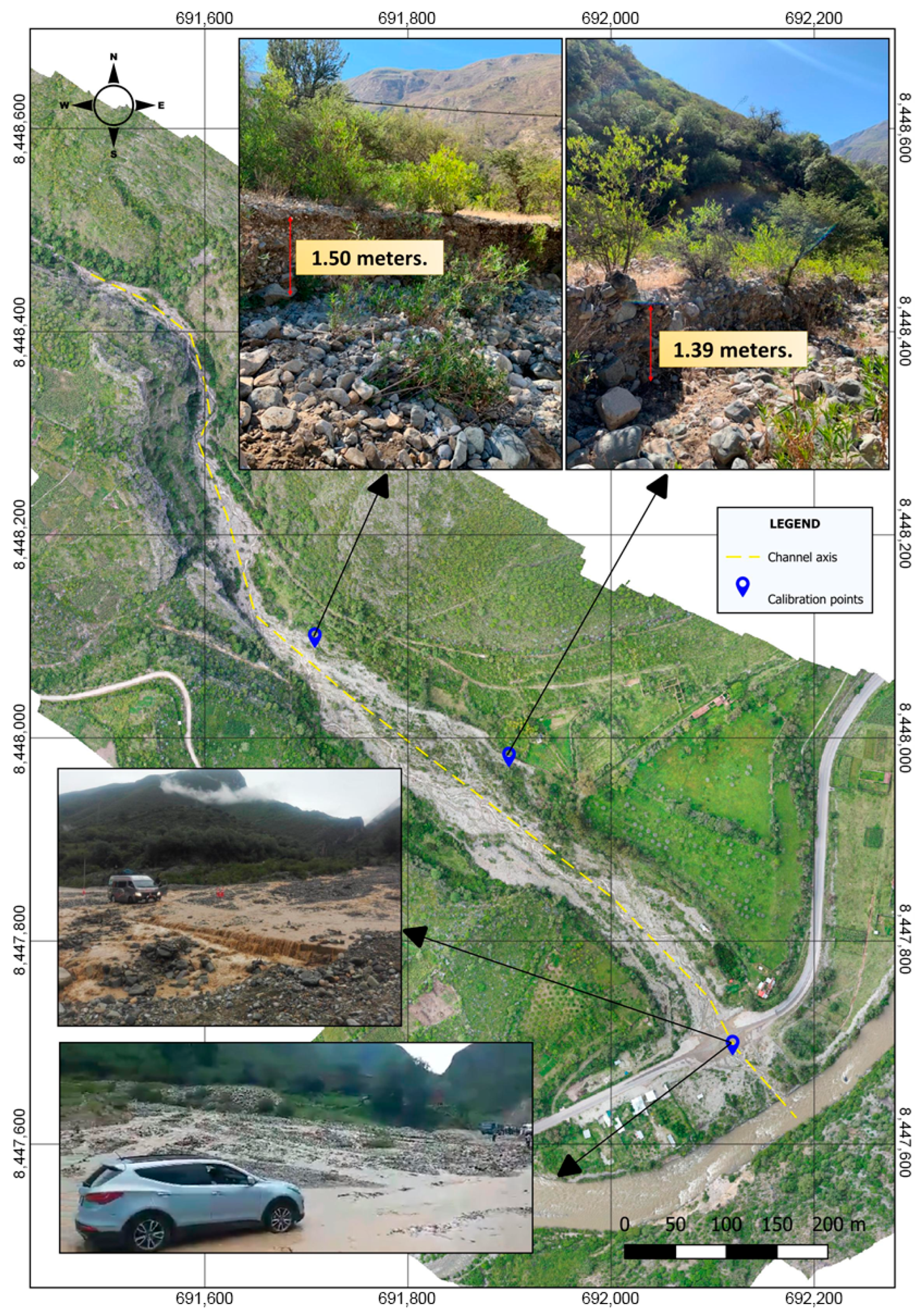
Accurately estimating the CV for non-Newtonian flows presents significant challenges. Current methodologies include comparative analysis of pre- and post-event LIDAR data or by deduction from historical records [33]. In this study, CV was estimated through an event that occurred in 2021, and through declarations from residents living near the stream.

3. Materials and Methods

The proposed methodology (Figure 1) for this study consists of the following steps:

• Study area definition: The Amoray Gully watershed was delineated using QGIS 3.16 software based on satellite imagery and a 5 m resolution DEM from the Earthdata platform. Key physiographic parameters (e.g., area, slope, main channel length) were extracted for hydrologic modeling.
• Hydrological processing: Maximum 24 h rainfall records from three nearby SENAMHI meteorological stations [37] (Andahuaylas, Tambobamba, and Chalhuanca) [37] were analyzed for the 1996–2020 period. A rainfall frequency analysis was carried out using the HIDROESTA software [38], applying the Kolmogorov–Smirnov goodness-of-fit test to identify the best-fitting statistical distribution (e.g., Log-Pearson Type III, Gumbel, Log-Normal). Design storm hyetographs for return periods of 2, 5, 10, 25, 50, 100, 200, and 500 years were generated using Dick Peschke’s Alternating Block Method. Rainfall-runoff transformation was performed in HEC-HMS using the Soil Conservation Service (SCS-CN) method. Curve Number (CN) values were derived from a raster model provided by the National Water Authority of Peru (ANA), based on land use and hydrologic soil group classifications [39]. No baseflow contribution was considered in the model due to the torrential behavior of the watershed.
• Terrain and soil data collection: A drone-based photogrammetric survey was used to generate a high-resolution Digital Elevation Model (DEM). Field reconnaissance was conducted to assign Manning’s roughness coefficients to different land cover types, following the guidelines of Chow [36]. Soil samples were collected from three test pits at 1.5 m depth and classified using USCS. Granulometric analyses were performed to estimate rheological parameters for non-Newtonian flow modeling in HEC-RAS.
• Hydraulic modeling in HEC-RAS: Two-dimensional simulations were performed in HEC-RAS 6.6 using both Newtonian and non-Newtonian flow assumptions. The hydrodynamic model was calibrated using the 2021 debris flow event reported by INDECI [40], supported by photographic evidence and field validation of watermarks. Peak flows from HEC-HMS corresponding to return periods of 5, 50, and 100 years were used as input. Rheological parameters were incorporated according to empirical equations defined by HEC-RAS [30], assuming a Typical Soil behavior. Comparisons were made between flow depths, velocities, and flood extents for Newtonian and non-Newtonian simulations.
• Infrastructure design: Based on the results of the 100-year scenario, a culvert structure was designed using HY-8 software to prevent blockage of the national highway crossing the alluvial fan. The design adheres to Peruvian technical guidelines for flood mitigation infrastructure [41].

Additionally,

Table 3. Data sources and processing methodology.

No.	Variable/Data	Type	Model Usage	Source/Tool	Description/Notes
1	Watershed physiographic parameters	Input	Study area definition	EarthData NASA (5 m DEM) [42], QGIS 3.16 [43]	Watershed delineation, calculation of area, slope, and main channel length.
2	Topography (5 cm DEM)	Input	Study area definition	RTK drone photogrammetry	High-resolution terrain model for hydraulic modeling.
3	24 h maximum rainfall	Input	Hydrological processing	SENAMHI (Tambobamba, Chalhuanca, Andahuaylas stations) [37]	1996–2020 series used for frequency analysis and isohyet generation with HIDROESTA.
4	Rainfall frequency analysis	Processing	Hydrological processing	HIDROESTA [38]	Software for statistical distribution fitting and isohyet computation.
5	Design hyetographs	Intermediate	Hydrological processing	MTC Hydrology Manual (Alternating Block Method) [32]	Construction of synthetic hyetographs for different return periods.
6	Curve Number (CN)	Input	Hydrological processing	ANA raster (land use + hydrologic soil group) [39]	CN calculation under normal, dry, and wet antecedent moisture conditions.
7	Rainfall-runoff transformation	Intermediate	Hydrological processing	SCS-CN Method (HEC-HMS) [44]	Empirical method for ungauged watersheds.
8	Water marks/rainfall duration	Input	Hydrological processing	Field observations	Used to validate the 2021 debris flow event.
9	Manning’s roughness coefficients	Input	Terrain and soil data	Field inspection + standard tables [45]	Values based on channel and surface type.
10	Rheological parameters	Input	Terrain and soil data	Laboratory tests + HEC-RAS documentation [33]	Yield stress and dynamic viscosity for hyper concentrated flows.
11	Non-Newtonian flow characterization	Validation	Hydraulic modeling	INDECI [40]	2021 event classified as a debris flow (huayco) used for model calibration.
12	Hydraulic modeling (2D flow)	Processing	Hydraulic modeling	HEC-RAS 6.6 [46]	Simulation of Newtonian and non-Newtonian flow conditions.
13	Culvert design	Output	Infrastructure design	HY-8 v7.7 [47] + Peruvian road standards [32,41]	Design of cross-drainage structure compatible with the national highway.

outlines the sources/tools, types, descriptions, and model usage of the data used in this research.

4. Study Area

The Amoray Gully, framed between the headwaters of the Llehua River of constant course and the Antapacca Gully of permanent course, is placed in the southern zone of Peru, in the district of Colcabamba, province of Aymaraes, Apurimac region. Geographically, it is located by the following UTM coordinates: South (S): 8,450,682 m; West (W): 689,213 m; Altitude: 3360 masl (meters above sea level). The location of the study area is shown in Figure 2.

Watershed Analysis

The delimitation of the watershed corresponding to Zone 18S (Figure 3) was carried out using the QGIS 3.16 software [43], subsequently a digital model of the Earthdata database [42] with a resolution of 5 m was used, obtaining the most important physiographic parameters of the micro basin (

Table 4. Summary of physiographic parameters of the micro-basin QGIS.

Physiographic Parameters of the Micro-Basin
WGS 1984 UTM Z 18S
Parameters	Value	Unit
Area	33.52	km2
Perimeter	39.96	km
Maximum elevation	4432.00	masl
Minimum elevation	2432.00	masl
Difference in elevations	2000.00	m
East coordinate starting point	692,170.80	m
North coordinate starting point	8,447,689.70	m
Centroid X	687,882.98	m
Centroid Y	8,452,514.03	m
Main channel length	11.90	km

).

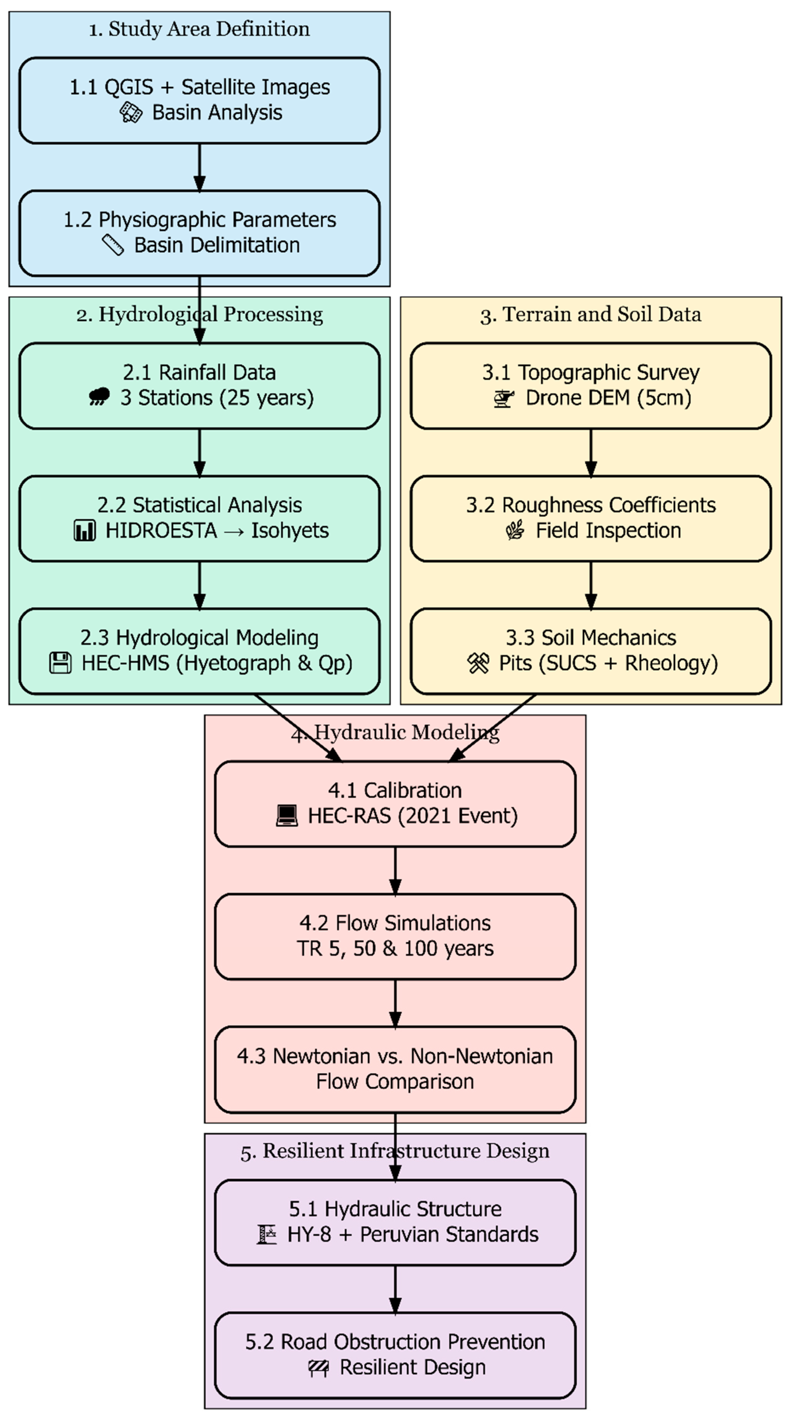
5. Hydrological Processing

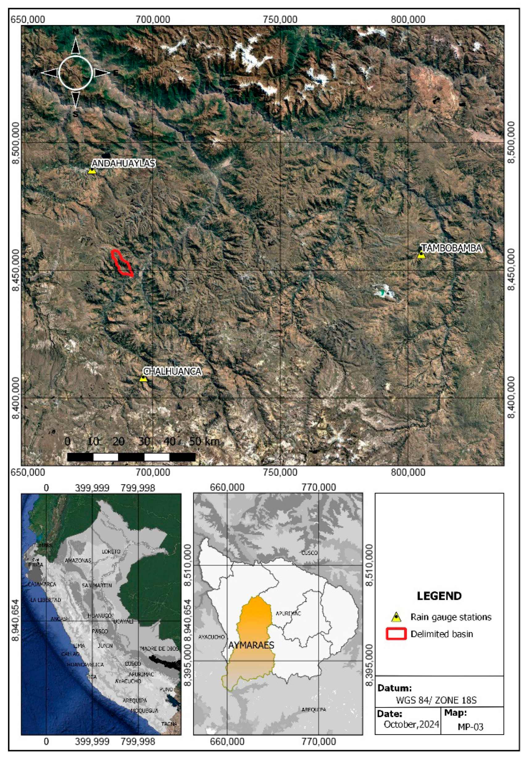
Precipitation data from the nearest stations to the study area, which are the Tambobamba, Chalhuanca, and Andahuaylas stations (Figure 4), were used, obtaining maximum 24 h precipitation records from 1996 to 2020, from the National Meteorology and Hydrology Service of Peru-SENAMHI. The analysis and processing of the information was performed from the historical data of the maximum 24 h precipitation of each station, using the Smirnorv–Kolgomorov goodness-of-fit test; then, the precipitation was calculated for each return period of 2, 5, 10, 25, 50, 100, 200, and 500 years with a significance level of α = 0.05, with the assistance of the HIDROESTA 2.0. software [38], which uses the parameters considered by the Peruvian regulations [32]. The maximum rainfall in 24 h for the mentioned return periods is shown in

Table 5. Maximum rainfall in 24 h (mm), for different return periods at each station.

Return Period	Station
RP (years)	Andahuaylas	Tambobamba	Chalhuanca
	Log Pearson type III	Gumbel	Log-normal 3 parameters
2	27.08	37.49	32.68
5	32.67	45.69	39.86
10	36.26	51.13	45.08
25	40.72	57.99	52.14
50	44.00	63.09	57.7
100	47.27	68.14	63.52
200	50.52	73.18	69.62
500	54.85	79.83	78.15

. The 1000-year return period was excluded due to the lack of regulatory requirements and the high associated costs, which are only justifiable for critical infrastructure, such as large dams or nuclear facilities. Instead, the 500-year return period was considered a technically adequate extreme scenario.

Therefore, the maximum annual 24 h rainfall is calculated using the isohyet method for each return period, as shown in

Table 6. Maximum annual rainfall in 24 h—isohyet method.

RP (Years)	Maximum Annual Rainfall in 24 h (mm)
2	30.29
5	36.79
10	41.26
25	47.10
50	51.58
100	56.13
200	60.86
500	67.36

.

For the determination of the liquid hydrographs, the Dick Peschke methodology and the alternating block method were used, and the calculation of the curve number factor was obtained through the raster model of the Peruvian entity Autoridad Nacional del Agua (ANA). In Peru, ANA is a public institution of the Ministry of Agriculture and Irrigation in charge of the administration of natural sources and water volumes, which contains the use and type of soil in wet, dry, and normal conditions [48]. For the rainfall-runoff transformation, the hydrologic model of the HEC-HMS software was used, which uses the Soil Conservation Service (SCS) [49].

Table 7. Input data—Quebrada Amoray.

Description	Area (km2)	Curve Number	Concentration Time (h)
Quebrada Amoray	33.52	85	2.9

shows the input data to the HEC-HMS hydrologic model.

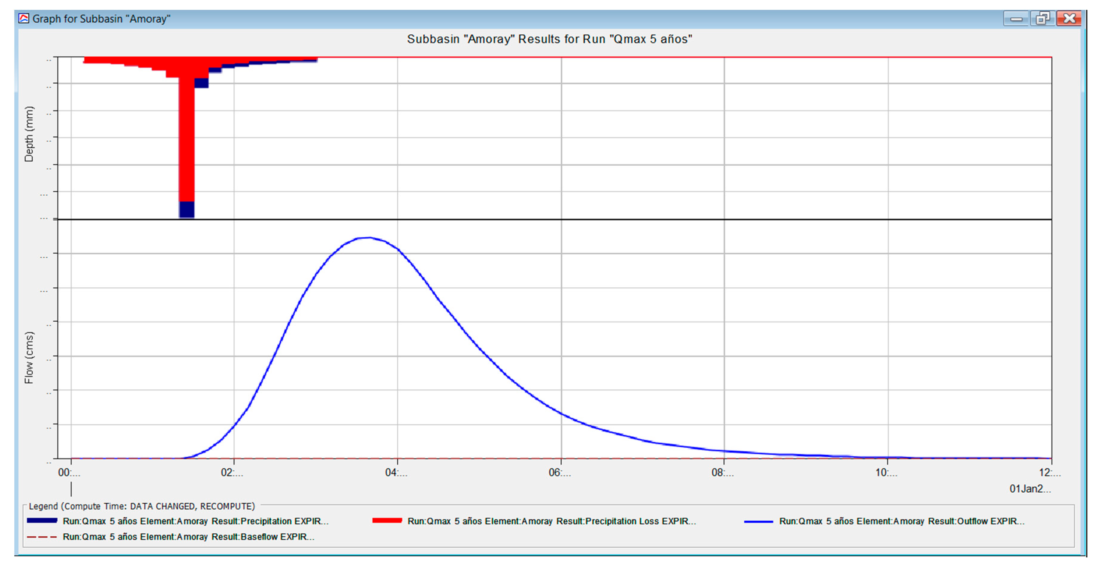
The maximum instantaneous discharges for the 5-year return period (Figure 5) and the different return periods (

Table 8. HEC-HMS flow rate results.

Return Period RP (Years)	Maximum Flow $({\mathbf{m}}^3/\mathbf{s}$)
2	8.8
5	12.9
10	17.6
25	24.2
50	30.3
100	37.6
200	46.2
500	59.9

) are also shown.

6. Hydraulic Processing

6.1. Topography

The photogrammetric survey consists of obtaining data such as contour lines and orthophotos using a drone, and the establishment of a static point, which is performed through the post-processing of the horizontal and vertical correction of the photographs, reaching an accuracy ranging from 2 to 5 cm, which must be linked to the national geodetic network. For this study, fieldwork was conducted using an RPAS RTK drone. Considering the shape and area of interest, the plan was developed, and four flights were carried out over the Amoray alluvial fan. Figure 6 shows the positions of the cameras and the orthophoto of the Amoray Gully.

6.2. Roughness Coefficients

Determining the Manning roughness coefficients is one of the most important steps in flood modeling, as these coefficients directly influence flood extents, water levels, and flow velocities [50]. To ensure spatial accuracy in the study area, the HEC-RAS land cover layer methodology [51] was employed. This approach provides detailed spatial representation of different ground cover types. The method involves (1) generating specific classification polygons, (2) assigning Manning’s coefficients tailored to each cover type (in this case, primarily the channel bed, as it is a natural gully), and (3) integrating them with the digital terrain model. This methodology significantly improves hydraulic model accuracy by accounting for the actual spatial distribution of roughness, avoiding oversimplifications in non-urbanized natural environments.

To find Manning coefficients, the roughness values of Ven Te Chow [45] were considered, which are shown in

Table 9. Roughness coefficients Quebrada Amoray.

N°	Component	Manning’s Number
		Description	“n”
Manning #1	Baden	Unpolished	0.017
Manning #2	Panamericana Highway	Rough asphalt	0.016
Manning #3	Main channel	Meanders with some rocks and grasses	0.045
Manning #4	Buildings	Clean Soil	0.022
Manning #5	Cultivation area	Short grass	0.035

based on the components found in the field. The recognition and assignment of the roughness coefficients were conducted in situ with support from orthophotos and the results are shown in Figure 7.

6.3. Soil Mechanics Study

For the soil mechanics tests, in situ samples were taken in three (03) pits with a depth of 1.5 m to establish the rheological parameters. The sample N° 1 was obtained at the beginning of the alluvial fan; this is a model sample, since the purest mixture is found at the beginning, from which the rheological parameters are derived [52]. Samples N° 2 and N° 3 were obtained from the middle part of the stream bed and from the end of the alluvial fan. After being analyzed in the laboratory, samples N° 1, N° 2, and N° 3 were found to have a USCS classification “SP” (poorly gravelly sand).

6.4. Obtaining Rheological Parameters

To obtain the rheological parameters (yield strength and dynamic viscosity), the exponential, user yield, and user-defined viscosity approximations were used. HEC-RAS adds limits and ranges for the rheological parameters [33], according to the type of soil material [27], as it is shown in

Table 10. Yield stress coefficients [33].

Type	Liquid Limit CV	a	b	Range (Pa)
Typical Soil	65–80%	0.005	17.2	375–5000
Kaolinite	40–50%	0.05	20.7	200–1600
Sensitive Clays	35–60%	0.3	23.0	960–300 k
Bentonite	5–20%	0.002	230.3	200–2 × 1017

and

Table 11. Dynamic viscosity coefficients [33].

Type	Liquid Limit CV	B	Range (Pa-s)
Typical Soil	65–80%	18.4	160–2500
Kaolinite	40–50%	18.4	200–1600
Sensitive Clays	35–60%	11.5	0.1–1
Bentonite	5–20%	230.3	100–1 × 1017

.

According to the results of the granulometric study, it is assumed that the soil of the Amoray Gully is Typical Soil. Subsequently, the rheological parameters were calculated with the empirical equations provided by HEC-RAS (Equations (5) and (6)). These are shown in

Table 12. Rheological parameters—Amoray Gully.

Volumetric Concentration	Yield Stress	Dynamic Viscosity
61–65.5%	390.6 Pa	171.44 Pa-s

.

7. Hydraulic Modeling in HEC-RAS

For the modeling of the Newtonian flow in HEC-RAS, a georeferenced digital elevation model (DEM) was used (Figure 8), which was added in the RAS MAPPER option of the software. Then the perimeter of the study area was created, with a 5 × 5 computational mesh; afterward, the boundary conditions were created, and finally, the HEC-HMS liquid hydrograph was added, so the program can execute the processing. For a non-Newtonian flow, the simulation criteria are the same; once the rheological parameters are known, they are added in the “unsteady flow data” option of HEC-RAS.

The DEM study area was delineated based on the following: the critical maximum flood point along the main roadway at the low-water crossing (baden)—an engineered structure designed to permit surface flow during flood events, with elevation flush with or below the natural channel bed; a 1 km upstream section encompassing the alluvial fan apex (sediment transport-to-deposition transition zone); and an extended reach for comprehensive Newtonian/non-Newtonian flow regime analysis, surpassing the 500 m minimum requirement established by Peruvian regulations [32]. It should be noted that the DEM has not undergone terrain modifications or deletions, maintaining the natural and current ground conditions.

Calibration of the Model with Field Evidence

To support the reliability of the model results, it is necessary to calibrate the simulation [53]. For calibration, the event that occurred in the year 2021 was used, where the Amoray Gully witnessed debris flows according to the reports of the Peruvian entity INDECI (National Institute of Civil Defense) [40]. First, the design flow was calibrated through three simulations for the return periods of 2, 5, and 10 years, where the liquid flow of 12.9 m³/s (5-year return period) is the flow that resembles the mentioned event. Also, the volumetric concentration was estimated according to the images taken of the event (Figure 9) and with the testimonies of the villagers living near the study area; the volumetric concentration was estimated at 61% and a maximum of 65.5%.

The calibration of the maximum streamflow was performed with the evidence left in the field [22]; this method consists of adjusting the model’s streamflow with the fluid footprint left by the stream [54]. For this study, points were taken at the beginning and in the middle part of the stream’s alluvial fan, where it was verified that the fluid footprint left by the stream reached a height of 1.39 m and 1.50 m, as shown in Figure 9.

These results are verified with the first model, which presents a better fit to the given event of the year 2021. It must be considered that the debris flow parameters are very sensitive. In this context, it is important to make comparisons with field tests [22].

8. Results

8.1. Simulated Scenarios

Three simulations were performed to present the liquid hydrographs with return periods (RP) of 5, 50, and 100 years [22]. Subsequently, for the calculation of the debris flow, the calculation methodology of the empirical expression “O’BRIEN” was used, which is based on a “Bulking factor” that is a multiplier to the clear water flow [23].

8.1.1. Return Period (RP = 5 Years)

This first simulation was carried out with a design flow of 12.9 m³/s, for a return period of 5 years and a volumetric solids concentration of 65.5%, the results of which are shown in

Table 13. Results—RP = 5 years.

Type of Flow	Volumetric Concentration	Maximum Depth	Maximum Velocity	Flow Rate	Flood Area
Newtonian	-	3.92 m	4.38 m/s	$12.90{\mathrm{m}}^3/\mathrm{s}$	$0.00217{\mathrm{k}\mathrm{m}}^2$
Non-Newtonian	65.5%	4.57 m	2.03 m/s	$37.39{\mathrm{m}}^3/\mathrm{s}$	$0.00385{\mathrm{k}\mathrm{m}}^2$

and Figure 10, Figure 11, Figure 12 and Figure 13.

Additional maximum velocity and depth results from HEC-RAS can be visualized through profile lines, as shown in Figure 14 and Figure 15. The selected cross-section is located approximately 250 m upstream of the baden, where the channel exhibits uniform geometry and stable hydraulic conditions, making this location ideal for comparative performance analysis of the model outputs. The plots clearly demonstrate that non-Newtonian flows exhibit lower velocities compared to Newtonian flows, attributable to their higher density relative to clear water.

8.1.2. Return Period (RP = 50 and 100 Years)

The second and third simulations were carried out based on ANA regulations. The ANA, in its resolution N° 153-2016 (Regulation for the Delimitation and Maintenance of Marginal Limits in River Courses and Natural and Artificial Water Bodies) [55], indicates the return period of 50 years for natural watercourses adjacent to agricultural land and a return period of 100 years for natural watercourses next to population settlements. The comparison of results between the different return periods is shown in

Table 14. Results for TR = 50 and 100 years.

RP (Years)	Flow Type	CV	Maximum Velocity	Maximum Depth	$\mathbf{Flood}\mathbf{Area}({\mathbf{k}\mathbf{m}}^2)$
50	Newtonian	-	6.28 m/s	5.00 m	0.00275
100	Newtonian	-	6.65 m/s	5.07 m	0.00294
50	Non-Newtonian	65.5%	3.22 m/s	5.56 m	0.00578
100	Non-Newtonian	65.5%	3.54 m/s	5.70 m	0.00818

.

8.2. Cross-Section Works

According to the problems of the study area, a cross-section culvert (Multiplate Circular Culvert) was designed using the HY-8 program. For its design, the results of the maximum drainage of the 50-year return period were used, which, according to the manual of Hydrology, Hydraulics and Drainage in Peru, the return period is 50 years [32]. For the selection of the culvert diameter, the technical data sheet of a local company was used. The culvert consists of five barrels, a diameter of 2.12 m, and model 28C [56]; the front and side view of the culvert are visualized in Figure 16 and Figure 17.

9. Conclusions

The HEC-HMS model was employed to determine peak discharges in the Amoray Gully through precipitation-runoff transformation via SCS Unit Hydrograph and a Net rainfall estimation using the Curve Number method (CN = 85). The model showed sensitivity to the concentration time parameter (2.9 h), yielding peak flows for multiple return periods.

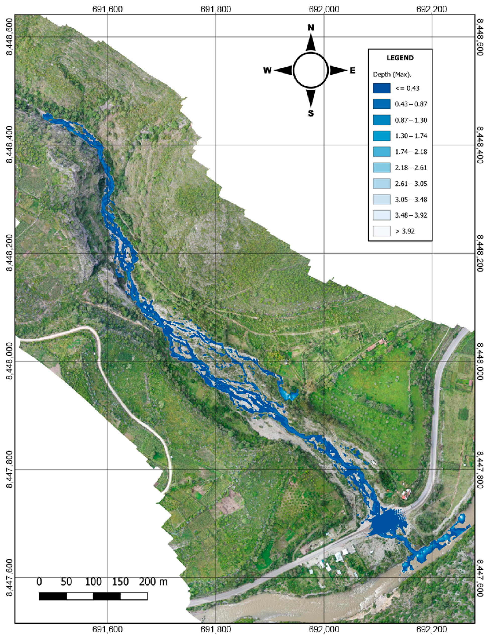
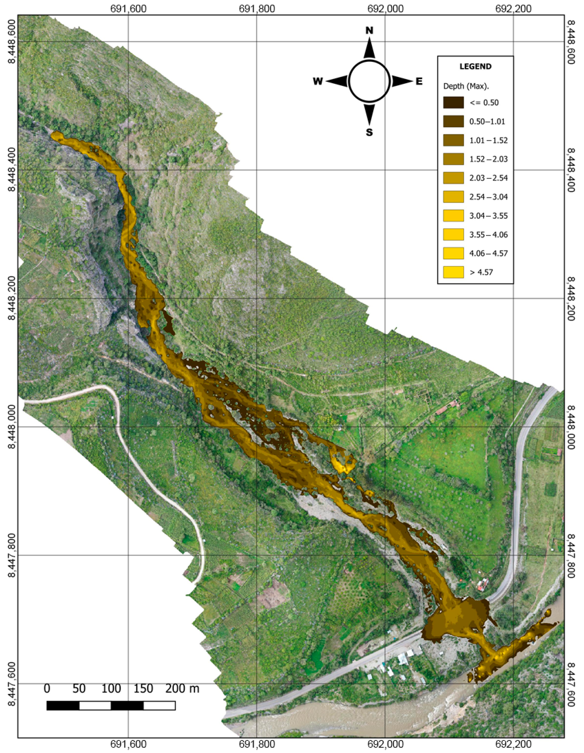
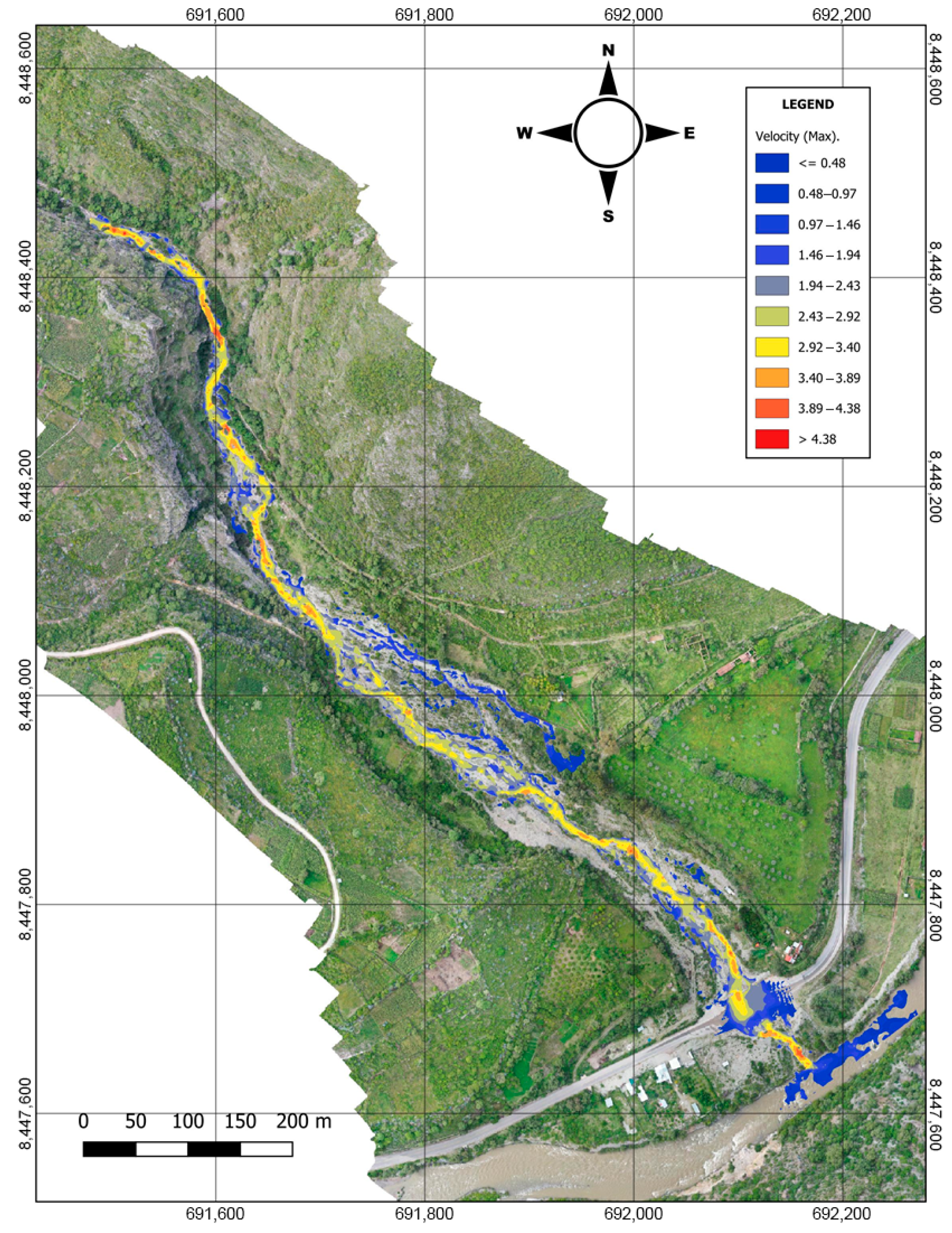
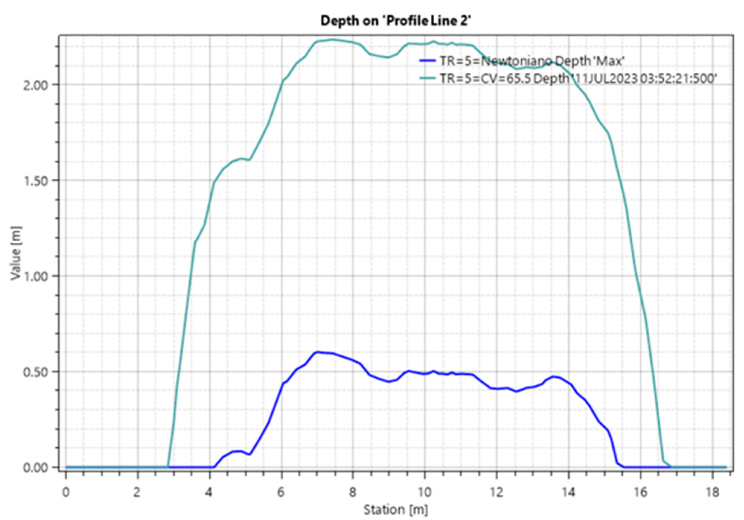
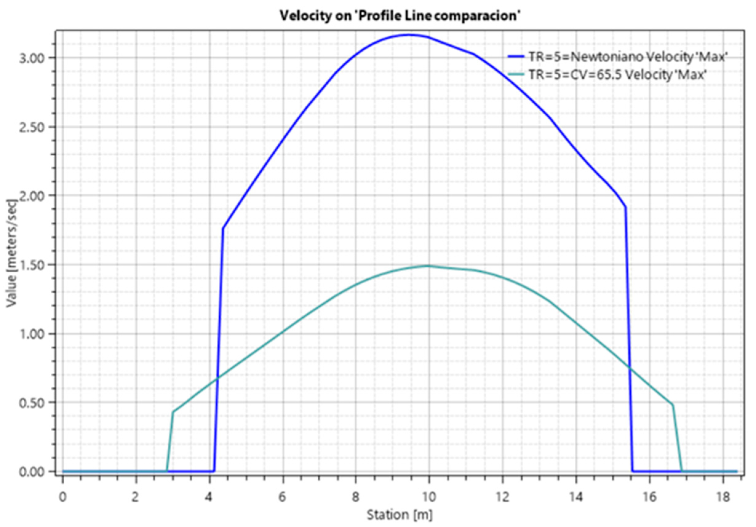
The HEC-HMS/HEC-RAS 6.6 coupled framework demonstrates superior flood risk assessment in alluvial fans, revealing that traditional clear-water models underestimate flood depths by 17%, and conventional approaches overestimate flow velocities by 54% for 5-year return period events. These discrepancies, evidenced in the 2021 Amoray Gully disaster, jeopardize infrastructure resilience when designed with outdated methods.

The O’Brien rheological model (CV = 61–65.5%) successfully captured debris flow dynamics, offering local municipalities in sediment-rich environments a validated methodology that addresses a critical gap in the country’s current hydraulic design standards [29], which lack provisions for non-Newtonian flows.

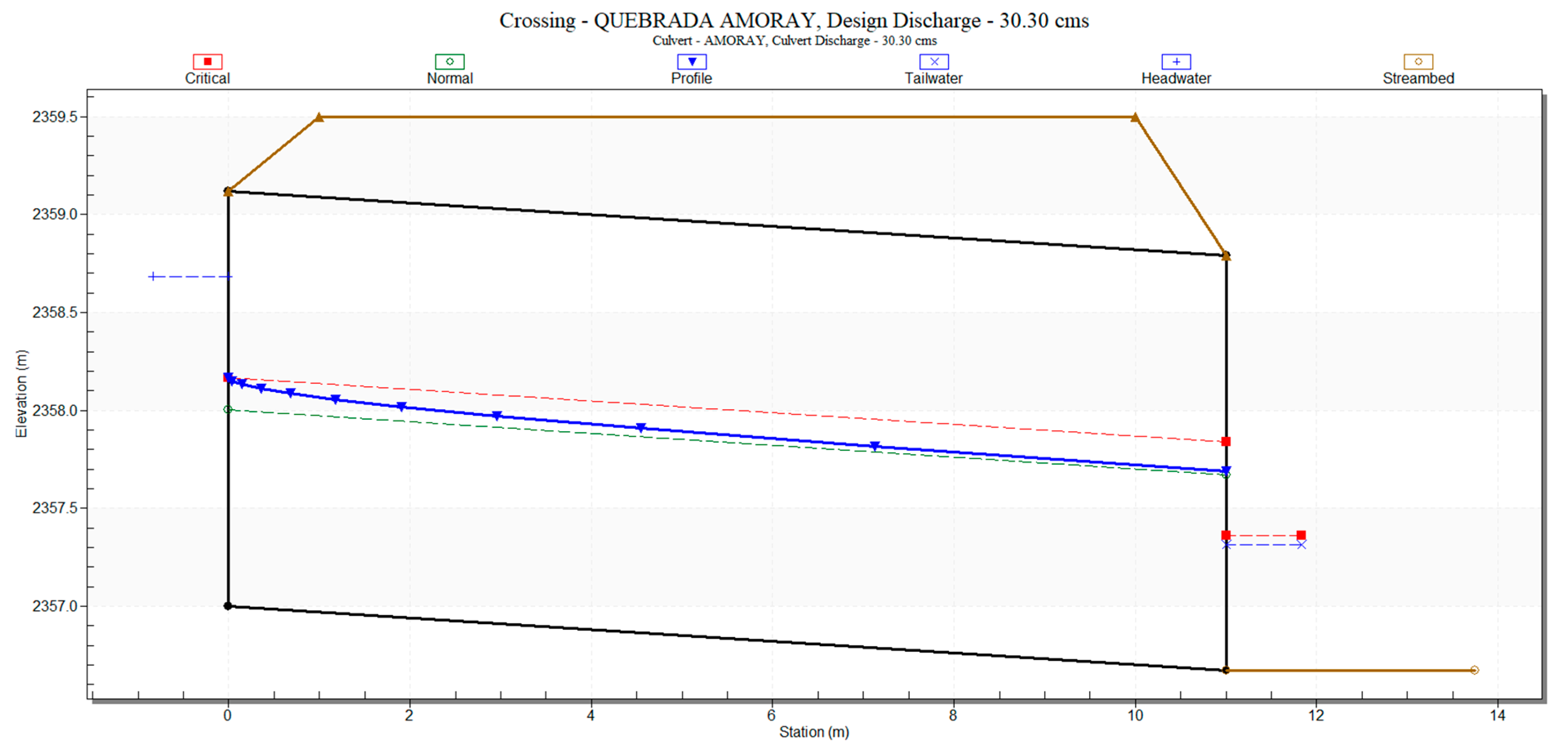
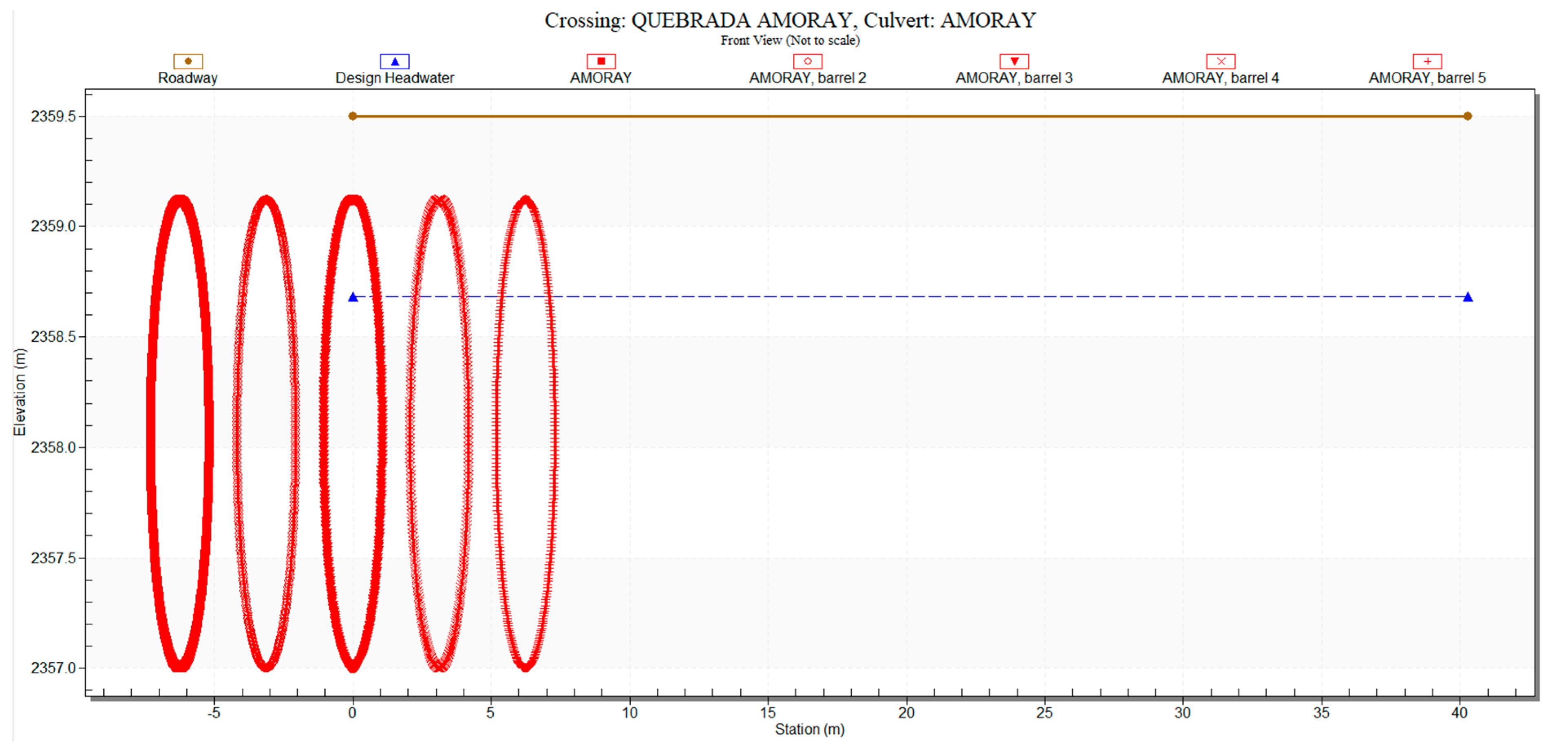
A circular multi-eye, multi-plate culvert (5 units of ∅2.12 m) was designed in compliance with Peruvian standards [32], specifically to mitigate obstruction risks from debris flows during extreme events (50-year return period) at the Amoray Gully (km 35 of the Lima–Abancay Highway). This structure features a trapezoidal section (downstream), eaves, and end walls with square edges. This technical solution, implemented in alluvial fans, is scalable for protecting critical road infrastructure, and offers potential application in similar geomorphological contexts.

Developing countries should mandate non-Newtonian modeling for infrastructure in debris-flow-prone areas, as demonstrated by the catastrophic failures during the 2016–2017 El Niño phenomenon [17].

The incorporation of HEC-RAS modeling outputs with real-time debris flow monitoring networks in high-risk gullies would substantially enhance urban preparedness and early warning systems. The implementation of additional control structures such as check dams should be considered to manage debris flows, taking into consideration climate change impacts, potential cascade failures of check dams due to unprecedented debris flows, dynamic forces, and rock impacts [57].

The hydraulic modeling methodology presented is useful for government authorities for adequate flood control and can be replicated in other countries with similar considerations [58], and, thus, seeking resilience in hydraulic infrastructures in terms of hydraulic modeling facing hydrological phenomena [59].

Furthermore, the model can be recalibrated in future studies using specialized hydraulic modeling technologies and software such as sediment transport modules in HEC-RAS and Iber, specifically through advanced analysis of sedimentological parameters (e.g., volumetric concentration), and the processing of new hydrological records. This update capability will progressively optimize the accuracy of numerical simulations.

References

1. Watson, G.; Ahn, J.E. A Systematic Review: To Increase Transportation Infrastructure Resilience to Flooding Events. Appl. Sci. 2022, 12, 12331. [Google Scholar] [CrossRef]
2. Department of Environmental Conservation. Flood Resilience. Available online: https://dec.vermont.gov/content/flood-resilience (accessed on 18 March 2025).
3. Zhao, H.; Wang, H.; Zhang, Y.; Zhao, R.; Qi, Z.; Zhang, H. Flash Flood Simulation for Hilly Reservoirs Considering Upstream Reservoirs—A Case Study of Moushan Reservoir. Sustainability 2024, 16, 5001. [Google Scholar] [CrossRef]
4. CISA. Critical Infrastructure Sectors. Available online: https://www.cisa.gov/topics/critical-infrastructure-security-and-resilience/critical-infrastructure-sectors (accessed on 18 March 2025).
5. da Silva, L.A.; Rudorff, C.; Ovando, A.; Pimentel, A.; Cuartas, L.A.; dos Alvalá, R.C.S. Inundation Mapping Using Hydraulic Modeling with High-Resolution Remote Sensed Data: A Case Study in the Acre River Basin, Brazil. Model. Earth Syst. Environ. 2024, 10, 3051–3066. [Google Scholar] [CrossRef]
6. Ortiz-Giraldo, L.; Botero, B.A.; Vega, J. An Integral Assessment of Landslide Dams Generated by the Occurrence of Rainfall-Induced Landslide and Debris Flow Hazard Chain. Front. Earth Sci. (Lausanne) 2023, 11, 1157881. [Google Scholar] [CrossRef]
7. Vega, J.; Ortiz-Giraldo, L.; Botero, B.A.; Hidalgo, C.; Parra, J.C. Probabilistic Cascade Modeling for Enhanced Flood and Landslide Hazard Assessment: Integrating Multi-Model Approaches in the La Liboriana River Basin. Water 2024, 16, 2404. [Google Scholar] [CrossRef]
8. Alamanos, A.; Papaioannou, G.; Varlas, G.; Markogianni, V.; Papadopoulos, A.; Dimitriou, E. Representation of a Post-Fire Flash-Flood Event Combining Meteorological Simulations, Remote Sensing, and Hydraulic Modeling. Land 2024, 13, 47. [Google Scholar] [CrossRef]
9. Peker, İ.B.; Gülbaz, S.; Demir, V.; Orhan, O.; Beden, N. Integration of HEC-RAS and HEC-HMS with GIS in Flood Modeling and Flood Hazard Mapping. Sustainability 2024, 16, 1226. [Google Scholar] [CrossRef]
10. Samela, C.; Carisi, F.; Domeneghetti, A.; Petruccelli, N.; Castellarin, A.; Iacobini, F.; Rinaldi, A.; Zammuto, A.; Brath, A. A Methodological Framework for Flood Hazard Assessment for Land Transport Infrastructures. Int. J. Disaster Risk Reduct. 2023, 85, 103491. [Google Scholar] [CrossRef]
11. Ccanccapa Puma, J.; Hidalgo Valdivia, V.A.; Espinoza Vigil, A.J.; Booker, J. Preserving Heritage Riverine Bridges: A Hydrological Approach to the Case Study of the Grau Bridge in Peru. Heritage 2024, 7, 3350–3371. [Google Scholar] [CrossRef]
12. Huarca Pulcha, A.; Espinoza Vigil, A.J.; Booker, J. Prioritizing Riverine Bridge Interventions: A Hydrological and Multidimensional Approach. Designs 2023, 7, 117. [Google Scholar] [CrossRef]
13. Espinoza Vigil, A.J.; Booker, J. Hydrological Vulnerability Assessment of Riverine Bridges: The Bajo Grau Bridge Case Study. Water 2023, 15, 846. [Google Scholar] [CrossRef]
14. Zavala, K. Dr. Rodríguez: “Perú Es Uno de Los Países Más Vulnerables al Cambio Climático”>> UDEP Hoy. Available online: https://www.udep.edu.pe/hoy/2021/11/dr-rodriguez-peru-es-uno-de-los-paises-mas-vulnerables-al-cambio-climatico/ (accessed on 20 September 2024).
15. Organización Panamericana de la Salud Fenómeno El Niño, 1997–1998. Crónicas Desastres 2000, 2000, 175–230.
16. Servicio Nacional De Meteorologia E Hidrologia Del Peru Informe Técnico El Niño Costero 2017 Condiciones Termo-Pluviometricas a Nivel Nacional SENAMHI Peru 2017. Available online: https://sigrid.cenepred.gob.pe/sigridv3/documento/3656 (accessed on 5 July 2025).
17. Espinoza Vigil, A.J.; Booker, J.D. Building National Disaster Resilience: Assessment of ENSO-Driven Disasters in Peru. Int. J. Disaster Resil. Built Environ. 2023, 14, 423–433. [Google Scholar] [CrossRef]
18. INDECI Resumen Ejecutivo Historico-Temporada de Lluvias, 2016–2017. Available online: https://portal.indeci.gob.pe/emergencias/resumen-ejecutivo-historico-temporada-de-lluvias-2016-2017-actualizado-al-24-de-enero-2018-2/ (accessed on 26 January 2025).
19. INDECI Resumen Ejecutivo N° 323-2023. Temporada de Lluvias 2022–2023. Available online: https://drive.google.com/file/d/1TXLtyd6ne7oRen3-m3hrBYGD9rhL6Vzh/view (accessed on 26 January 2025).
20. El Peruano Decreto Supremo Que Declara El Estado de Emergencia En El Distrito de Chalhuanca de La Provincia de Aymaraes Del Departamento de Apurímac, Por Impacto de Daños a Consecuencia de Intensas Precipitaciones Pluviales-Decreto Supremo-N° 004-2024-PCM-Presidencia Del Consejo De Ministros. Available online: https://busquedas.elperuano.pe/dispositivo/NL/2256589-1 (accessed on 20 September 2024).
21. Salas, S.P.; Sellés, M.G.; i Plaza, J.B.; Melgar, L.I.G. Susceptibilidad a Inundación Por Flujos Torrenciales a Partir de La Integración Del Método Geomorfológico y de La Modelización Con FLO-2D, Lago Atitlán, Guatemala. Rev. Mex. Cienc. Geol. 2019, 36, 64–75. [Google Scholar] [CrossRef]
22. Quispe, R.L.; Vargas, E.P.; Jihuallanga, C.A. Nivel De Riesgo Por Desborde E Inundación Aplicando Un Modelo De Flujo De Escombros En La Quebrada Lluta Para La Mina Karla En Tacna. Cienc. Desarro. 2019, 23, 11–20. [Google Scholar] [CrossRef]
23. Del Savio, A.A.; Astocahuana, S.I.Q.; Navarro, L.F.C. Numerical Simulation of Debris Flows of the Catastrophic Event of February 2019 in Mirave-Peru. Rev. Ambiente Água 2019, 14, e2437. [Google Scholar] [CrossRef]
24. Hou, S.; Cao, P.; Chen, L.; Feng, Z.; Wang, L.; Li, A.; Liu, J.; Li, Y.; Zheng, H. Debris Flow Hazard Assessment of the Eryang River Watershed Based on Numerical Simulation. Hydrogeol. Eng. Geol. 2021, 48, 143–151. [Google Scholar] [CrossRef]
25. Martinez Olmedo, V.A. Aplicación y Comparación Modelos de Flujos Detríticos, FLO-2D y HEC-RAS a Quebradas Acerilla y La Mesilla, Cuenca Del Río Huasco, Eventos Marzo 2015. Bachelor’s Thesis, Universidad de Chile, Santiago, Chile, 2022. [Google Scholar]
26. Bonasia, R.; Turchi, A.; Madonia, P.; Fornaciai, A.; Favalli, M.; Gioia, A.; Di Traglia, F. Modelling Erosion and Floods in Volcanic Environment: The Case Study of the Island of Vulcano (Aeolian Archipelago, Italy). Sustainability 2022, 14, 16549. [Google Scholar] [CrossRef]
27. Gibson, S.; Moura, L.Z.; Ackerman, C.; Ortman, N.; Amorim, R.; Floyd, I.; Eom, M.; Creech, C.; Sánchez, A. Prototype Scale Evaluation of Non-Newtonian Algorithms in HEC-RAS: Mud and Debris Flow Case Studies of Santa Barbara and Brumadinho. Geosciences 2022, 12, 134. [Google Scholar] [CrossRef]
28. Masoumi, M.; Sarang, A.; Ardestani, M.; Niksokhan, M.H. Estimating Peak Flow of Farahzad River in Tehran under Climate Change and Debris Flow Scenarios: A Novel Approach and Its Implications for Urban Flood Hazard Mapping. J. Water Clim. Change 2024, 15, 1364–1379. [Google Scholar] [CrossRef]
29. Zahroni, A.; Nugroho, E.O.; Harlan, D.; Soentoro, E.A.; Aprilian, Z. Estimation of Debris Flow Using Curve Number Analysis for The Mount Agung Volcanic Event, Bali, Indonesia. E3S Web Conf. 2024, 476, 01015. [Google Scholar] [CrossRef]
30. Sanz-Ramos, M.; Bladé, E.; Sánchez-Juny, M.; Dysarz, T. Extension of Iber for Simulating Non–Newtonian Shallow Flows: Mine-Tailings Spill Propagation Modelling. Water 2024, 16, 2039. [Google Scholar] [CrossRef]
31. Wasklewicz, T.; Chen, A.; Guthrie, R.H. Post-Wildfire Debris Flow and Large Woody Debris Transport Modeling from the North Complex Fire to Lake Oroville. Water 2023, 15, 762. [Google Scholar] [CrossRef]
32. Ministerio de Transportes y Comunicaciones Manual de Hidrología, Hidráulica y Drenaje. Available online: https://spij.minjus.gob.pe/Graficos/Peru/2011/Octubre/10/RD-20-2011-MTC-14.pdf (accessed on 27 September 2024).
33. USACE Hydrologic Engineering Center HEC-RAS Mud and Debris Flow. Available online: https://www.hec.usace.army.mil/confluence/rasdocs/rasmuddebris (accessed on 5 October 2024).
34. Coussot, P. Mudflow Rheology and Dynamics. In Mudflow Rheol. Dyn.; IAHR Monograph Series; A.A. Balkema: Rotherdam, The Netherlands, 1997. [Google Scholar] [CrossRef]
35. O’Brien, J.S.; Julien, P.Y.; Fullerton, W.T. Two-Dimensional Water Flood and Mudflow Simulation. J. Hydraul. Eng. 1993, 119, 244–261. [Google Scholar] [CrossRef]
36. Herschel, W.H.; Bulkley, R. Konsistenzmessungen von Gummi-Benzollösungen. Kolloid-Z. 1926, 39, 291–300. [Google Scholar] [CrossRef]
37. Ministerio del Ambiente Perú SENAMHI-Descarga de Datos. Available online: https://www.senamhi.gob.pe/site/descarga-datos/ (accessed on 5 July 2025).
38. Villón, M. Hidroesta 2. Cálculos Hidrológicos. Segunda Ed.; Centro de Desarrollo de Material Bibliografico. Available online: https://isbn.cloud/9789968514163/hidroesta-2-calculos-hidrologicos-/ (accessed on 16 July 2025).
39. Geo GPS Perú: Numero de Curva-Descargar Mapa Shapefile. Available online: https://www.geogpsperu.com/2019/04/numero-de-curva-descargar-mapa.html (accessed on 5 July 2025).
40. Indeci Reporte Complementario No 7855-19/12/2021/Coen-Indeci/06:00 HORAS (Reporte No 1) Huaico en el Distrito de Colcabamba-Apurímac. Available online: https://portal.indeci.gob.pe/wp-content/uploads/2021/12/REPORTE-COMPLEMENTARIO-N%C2%BA-7855-19DIC2021-HUAICO-EN-EL-DISTRITO-DE-COLCABAMBA-APUR%C3%8DMAC-1.pdf (accessed on 5 October 2024).
41. Plataforma del Estado Peruano Resolución Jefatural N.° R.J. 332-2016-ANA-Normas y Documentos Legales-Autoridad Nacional Del Agua. Available online: https://www.gob.pe/institucion/ana/normas-legales/538418-r-j-332-2016-ana (accessed on 5 July 2025).
42. NASA Earthdata Search. Available online: https://search.earthdata.nasa.gov/search (accessed on 28 April 2025).
43. QGIS Web Site. Available online: https://qgis.org/ (accessed on 28 April 2025).
44. HEC-HMS User’s Manual. Available online: https://www.hec.usace.army.mil/confluence/hmsdocs/hmsum/latest (accessed on 6 July 2025).
45. Te Chow, V. Hidraúlica de Canales Abiertos; Mcgraw-Hill Interamericana: Bogotá, Colombia, 1994; ISBN 9586002284. [Google Scholar]
46. HEC-RAS Downloads. Available online: https://www.hec.usace.army.mil/software/hec-ras/download.aspx (accessed on 6 July 2025).
47. Culvert Hydraulics-Hydraulics-Bridges & Structures-Federal Highway Administration. Available online: https://www.fhwa.dot.gov/engineering/hydraulics/software/hy8/ (accessed on 6 July 2025).
48. Ramos, M.; Saldivar, G. Análisis de Riesgo Frente a Máximas Avenidas con el Uso del Producto Grillado Pisco pd en Las Quebradas Polanco, san Lázaro, Miraflores y Mariano Melgar en la Provincia de Arequipa; Universidad Catolica de Santa Maria: Arequipa, Peru, 2022. [Google Scholar]
49. Lee, K.K.F.; Ling, L.; Yusop, Z. The Revised Curve Number Rainfall–Runoff Methodology for an Improved Runoff Prediction. Water 2023, 15, 491. [Google Scholar] [CrossRef]
50. Demir, V.; Keskin, A.Ü. Obtaining the Manning Roughness with Terrestrial-Remote Sensing Technique and Flood Modeling Using FLO-2D: A Case Study Samsun from Turkey. Geofizika 2020, 37, 131–156. [Google Scholar] [CrossRef]
51. USACE Hydrologic Engineering Center HEC-RAS 2D User´s Manual-Creating Land Cover, Manning’s n Values, and % Impervious Layers. Available online: https://www.hec.usace.army.mil/confluence/rasdocs/r2dum/latest/developing-a-terrain-model-and-geospatial-layers/creating-land-cover-mannings-n-values-and-impervious-layers (accessed on 2 July 2025).
52. Puma, R.N.H.; Sivincha, F.C. Simulación de Huayco e Inundación y Propuesta de Solución En El Anexo de Pescadores, Distrito de Ocoña, Provincia de Camana, Departamento de Arequipa; Universidad Nacional de San Agustin: Arequipa, Peru, 2019. [Google Scholar]
53. Romero, S.L. Calibración de Un Modelo Hidráulico de Lluvia Distribuida En Una Cuenca: Procedimiento y Sensibilidad de Parámetros. Aplicación al Caso Del Río Ojailén (Ciudad Real); Dpto. Ingeniería Aeroespacial y Mecánica de Fluidos Escuela Técnica Superior de Ingeniería Universidad de Sevilla: Sevilla, Spain, 2023. [Google Scholar]
54. Flores, M.A.B. Análisis Comparativo de Un Modelo Hidrodinámico Unidimensional Para Flujo Newtonianos y No Newtonianos Del Río Seco Zona Urbana Tacna; Universidad Nacional Jorge Basadre Grohmann: Tacna, Peru, 2015. [Google Scholar]
55. ANA, R.J. No 153-2016-ANA; Drupal, Autoridad Nacional del Agua, Ministerio de Desarrollo Agrario y Riego: Lima, Peru, 2016. [Google Scholar]
56. Siderperu Ficha Tecnica Alcantarilla Multiplate. Available online: https://construyeconacerosiderperu.pe/productos/infraestructura-vial/alcantarillas/alcantarilla-multiplate-MP-152 (accessed on 5 October 2024).
57. Hosseinipoor, M.; Rudsary, A.M.; Danesh-Yazdi, M.; Kazempour, Z.; Yeganeh, Y. Why Structural Solutions for Flood Control Should Be Adapted to Climate Change? Nat. Hazards 2024, 121, 4657–4682. [Google Scholar] [CrossRef]
58. Juarez-Quispe, J.; Rojas-Chura, E.; Espinoza Vigil, A.J.; Guillén Málaga, M.S.; Yabar-Ardiles, O.; Anco-Valdivia, J.; Valencia-Félix, S. Advancing Sustainable Infrastructure Management: Insights from System Dynamics. Buildings 2025, 15, 210. [Google Scholar] [CrossRef]
59. Valencia-Félix, S.; Anco-Valdivia, J.; Espinoza Vigil, A.J.; Hidalgo Valdivia, A.V.; Sanchez-Carigga, C. Review of Green Water Systems for Urban Flood Resilience: Literature and Codes. Water 2024, 16, 2908. [Google Scholar] [CrossRef]
Figure 1. Methodology flow chart.
Water 17 02150 g001
Figure 2. Location map of the study area.
Water 17 02150 g002
Figure 3. Delimitation of the hydrographic basin—Amoray Gully.
Water 17 02150 g003
Figure 4. Location of rainfall stations.
Water 17 02150 g004
Figure 5. Liquid hydrograph-TR = 5 years.
Water 17 02150 g005
Figure 6. Positions of the cameras.
Water 17 02150 g006
Figure 7. Manning’s number—Quebrada Amoray.
Water 17 02150 g007
Figure 8. DEM Quebrada Amoray.
Water 17 02150 g008
Figure 9. Event 2021—Quebrada Amoray.
Water 17 02150 g009
Figure 10. Maximum depth—Newtonian flow.
Water 17 02150 g010
Figure 11. Maximum depth—non-Newtonian flow.
Water 17 02150 g011
Figure 12. Maximum velocity—Newtonian flow.
Water 17 02150 g012
Figure 13. Maximum velocity—non-Newtonian flow.
Water 17 02150 g013
Figure 14. Depth profiles: Newtonian and non-Newtonian flows (TR = 5 years). Y-axis: Depth (m); X-axis: Distance along profile (m).
Water 17 02150 g014
Figure 15. Velocity profiles: Newtonian and non-Newtonian flows (TR = 5 years). Y-axis: Velocity (m/s); X-axis: Distance along profile (m).
Water 17 02150 g015
Figure 16. Side view of the culvert.
Water 17 02150 g016
Figure 17. Front view of the culvert.
Water 17 02150 g017