Quasi-Optimized LSTM Approach for River Water Level Forecasting

Abstract

This study explores the application of a Long Short-Term Memory (LSTM) model for river water level forecasting, emphasizing the critical role of hyper-parameters optimization. Similar to physical and numerical rainfall-runoff models, LSTM relies on parameters to drive its data-driven modeling process. The performance of such models is highly sensitive to the chosen hyper-parameters, making their optimization essential. To address this, three algorithms—Grid Search, Random Search, and Bayesian Search—were applied to identify the most effective hyper-parameter combinations. Cross-correlation analysis revealed that average rainfall had a stronger influence on river water levels than upstream point rainfall, leading to its selection as the model input. The optimization focused on five key hyper-parameters: neuron units, learning rate, dropout rate, number of epochs, and batch size. Results showed that, while Grid Search required the most computational time, both Random and Bayesian Search were more efficient. Notably, Bayesian Search yielded the best predictive performance with minimal time cost, making it the preferred optimization method. Additionally, reproducible LSTM simulations were conducted to ensure the consistency and practical applicability of the forecasting in real-world scenarios. Overall, Bayesian Search is recommended for optimizing LSTM models due to its balance of accuracy and computational efficiency in hydrological forecasting.

1. Introduction

Floods are among the most devastating natural disasters, posing significant threats to human lives, property, and infrastructure. Accurate and timely flood forecasting is essential to mitigate these risks, providing authorities with critical information to implement preventative measures, allocate resources, and issue warnings. Traditional flood forecasting methods, such as hydrological models and numerical simulations, rely heavily on physical principles and detailed parameterization of complex watershed systems. However, these methods often require extensive calibration and are constrained by the availability and quality of input data. On the other hand, progress in artificial intelligence and machine learning has enabled data-driven methods like Long Short-Term Memory (LSTM) models, which have demonstrated strong potential in flood forecasting. Guo et al. [1] highlighted that machine learning models can serve as surrogate models to replace physically based flood simulations, under the assumption that these models are capable of learning the behavior of the target system even without explicitly representing the underlying physical processes, provided that sufficient and representative data are available. However, the authors also acknowledged limitations in their study due to the lack of large-scale flood datasets. This scarcity was attributed to the long computational time required for physically based simulations and the challenges associated with the widespread deployment of sensors for collecting observational data, both of which constrained the predictive performance of their CNN model. A recent study by Guglielmo et al. [2] introduced a novel approach for integrating physical principles into data-driven models, demonstrating enhanced predictive performance even when extrapolating beyond the training data boundaries or in data-scarce scenarios. This advancement suggests that applying data-driven models to real-world datasets from complex systems is becoming increasingly feasible and practical.

LSTM, a specialized type of recurrent neural network (RNN), has been widely used in sequence-based tasks due to its ability to capture long-term dependencies in data. This characteristic is particularly advantageous in hydrological forecasting, where the dynamics of rainfall-runoff processes exhibit temporal dependencies over extended periods. By learning patterns directly from historical data, LSTM models bypass the need for explicit physical equations, enabling them to model complex, nonlinear relationships between inputs (e.g., rainfall, temperature, and river flow) and outputs (e.g., water levels or discharge rates).

Despite its potential, the effectiveness of an LSTM model heavily depends on the selection of its hyper-parameters, which define the architecture and training process of the model. Hyper-parameters such as the number of neurons in the hidden layers, learning rate, dropout rate, batch size, and the number of training epochs significantly influence the model’s predictive accuracy, generalization ability, and training efficiency. The process of identifying the optimal combination of these hyper-parameters, known as hyper-parameter optimization, is crucial for achieving reliable flood forecasts.

Several optimization techniques have been developed to streamline the search for optimal hyper-parameters. Among these, Grid Search, Random Search, and Bayesian Optimization are commonly employed. Grid Search exhaustively evaluates all possible combinations of hyper-parameter values within a predefined range, ensuring a comprehensive search but often at a high computational cost. Random Search, on the other hand, samples hyper-parameter values randomly, providing a faster alternative with comparable performance in many cases. Bayesian Optimization uses a probabilistic model to guide the search for optimal hyper-parameters, balancing exploration and exploitation to identify promising configurations efficiently.

In the context of flood forecasting, the integration of these optimization algorithms into LSTM model development has demonstrated notable improvements in performance. For example, Bayesian Optimization has been shown to enhance model accuracy while reducing the time required for training, making it particularly suitable for time-sensitive applications like flood prediction. Additionally, the choice of input variables plays a critical role in the model’s success. For instance, variables such as average rainfall, point rainfall, upstream flow, and other meteorological parameters must be carefully analyzed to determine their relevance and correlation with the target variable. Selecting the most informative inputs ensures that the model captures the underlying hydrological processes effectively.

Recent studies have explored advanced techniques for improving flood forecasting and water level prediction. Long Short-Term Memory (LSTM) networks have shown promise in hydrological time series prediction [3], but their performance depends heavily on hyper-parameter selection [4]. To address this, researchers have applied various optimization methods. Particle Swarm Optimization (PSO) has been used to optimize LSTM hyper-parameters, improving flood forecasting accuracy and lead time [4]. Bayesian optimization algorithms have also been applied to enhance the performance of Extreme Gradient Boosting (XGB) models for flood susceptibility mapping [5]. Additionally, a hybrid model combining Random Search, LSTM, and Transformer architecture has shown promising results in rainfall-runoff simulation [6].

Ruma et al. [7] demonstrated the superiority of Long Short-Term Memory (LSTM) networks optimized with Particle Swarm Optimization (PSO) over traditional artificial neural networks (ANN) for water level forecasting in Bangladesh’s river network. Li et al. [8] proposed a hybrid approach combining a hydrodynamic model with ANN-based error correction, which significantly improved flood water level forecasting accuracy. This method optimized Manning’s roughness coefficients and used partial mutual information for input variable selection. Aditya et al. [9] compared the performance of ANN, adaptive neuro-fuzzy interference system (ANFIS), and adaptive neuro-GA integrated system (ANGIS) models for flood forecasting in India’s Ajay River Basin. Their results showed that the ANGIS model achieved the highest accuracy in predicting flood events. These studies highlight the potential of hybrid and optimized machine learning approaches in enhancing flood forecasting capabilities.

A noticeable gap exists in the current literature regarding the reproducibility of simulations using LSTM models. Most prior studies have primarily focused on evaluating the predictive performance of LSTM models, often overlooking the critical aspect of reproducibility. However, ensuring the consistency of a model’s predictive ability is essential for reliable real-world application, particularly in flood forecasting. Accurate and reproducible predictions are crucial for issuing timely and dependable flood warnings, which can significantly impact disaster preparedness and risk mitigation efforts.

This study focuses on optimizing an LSTM-based flood forecasting model by leveraging hyper-parameter optimization techniques. The target application is to predict river water levels at a specific station, a task that involves analyzing historical rainfall and water level data to make accurate and timely forecasts. Cross-correlation analysis is employed to identify the most influential input variables, ensuring the model incorporates only the most relevant data. Five key hyper-parameters—neuron units, learning rate, dropout rate, batch size, and number of epochs—are selected for optimization due to their significant impact on model performance.

To evaluate the effectiveness of different optimization techniques, three widely used algorithms—Grid Search, Random Search, and Bayesian Optimization—are applied to tune the LSTM model. The computational efficiency and predictive performance of the resulting models are compared to identify the most suitable approach for flood forecasting. Preliminary results indicate that, while Grid Search provides comprehensive coverage of the hyper-parameter space, it is computationally expensive. Random Search offers a faster alternative but lacks the systematic exploration of Bayesian Optimization, which consistently identifies optimal configurations with superior accuracy and efficiency.

The primary contribution of this research lies in providing actionable recommendations for the selection of input variables and optimization strategies aimed at developing robust and reliable flood forecasting systems. This is achieved by emphasizing the critical role of hyper-parameter optimization in enhancing the performance of LSTM models, supported by a comparative analysis of selected optimization techniques and an assessment of their respective strengths and limitations in practical applications. Apart from that, this study integrates the optimization of LSTM models using Grid Search, Random Search, and Bayesian Optimization into water level prediction, emphasizing not only traditional stochastic simulation but also reproducible simulation. The objective is to address the current research gap by presenting and discussing a comprehensive framework for LSTM-based flood forecasting that ensures reproducibility of results, an essential yet often overlooked aspect in existing studies.

The growing frequency and intensity of floods due to climate change underscore the need for advanced forecasting tools capable of providing accurate and timely predictions. LSTM models, when combined with effective hyper-parameter optimization techniques, represent a promising solution for addressing this challenge. By leveraging data-driven approaches and integrating optimization algorithms, this study aims to improve the accuracy, efficiency, and reliability of flood forecasts, contributing to enhanced disaster preparedness and resilience in vulnerable regions.

2. Study Area and Data Used

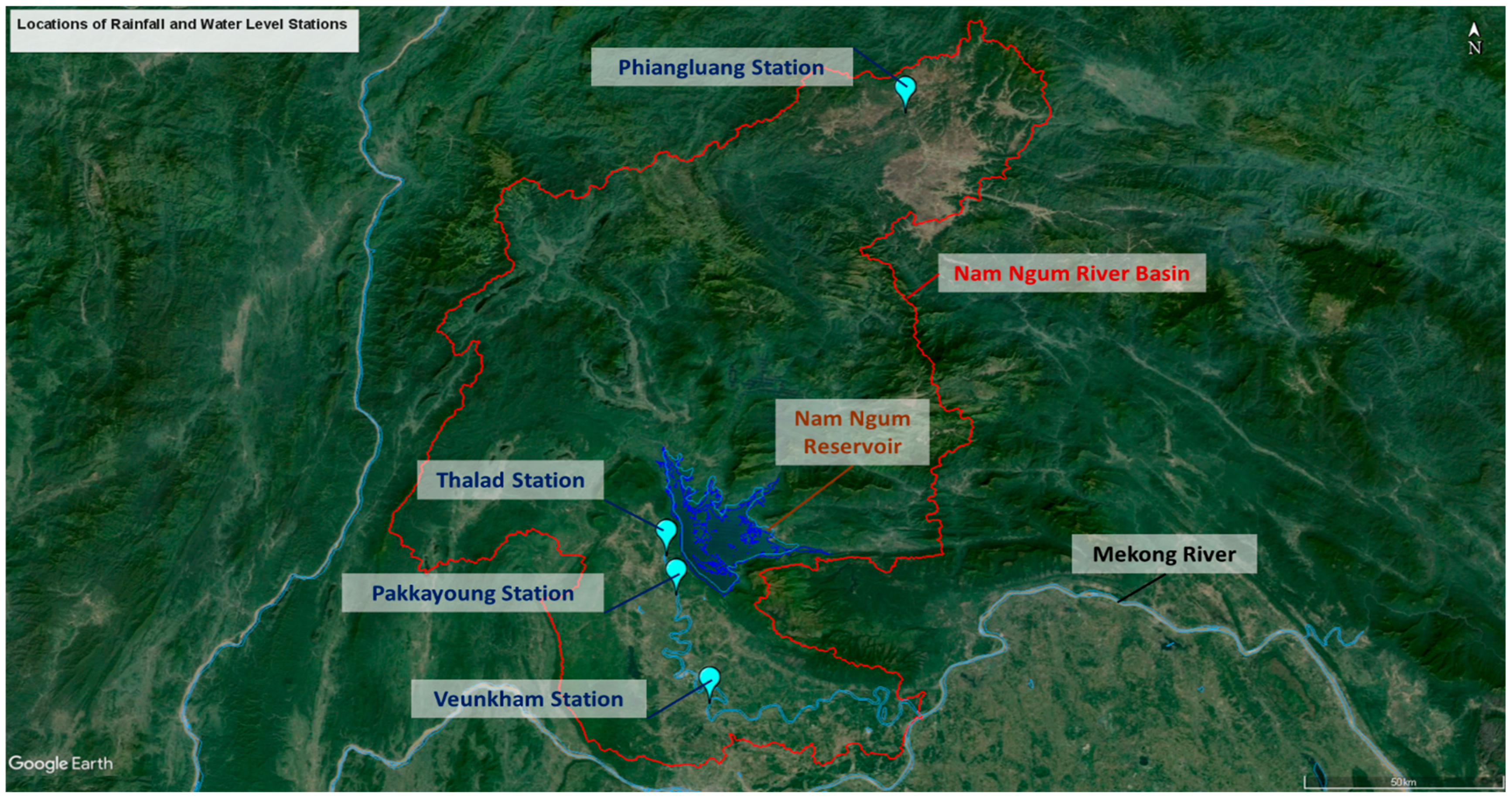
The Nam Ngum River Basin represents a critical natural asset for the Lao People’s Democratic Republic, significantly contributing to the nation’s food security. The basin’s principal watercourse, the Nam Ngum River, originates in the northeastern region and flows southward over a distance of approximately 420 km before converging with its major tributary, the Nam Lik River. After this confluence, the Nam Ngum River ultimately drains into the Mekong River at Pak Ngum. Covering a total catchment area of around 17,000 km², delineated by the red boundary in Figure 1, the basin receives an average annual rainfall of about 2000 mm, with variations ranging from 1200 mm to 3500 mm. The wet season typically spans from June to October, followed by a distinct dry season for the remainder of the year. On average, the Nam Ngum River Basin contributes approximately 21,000 million cubic meters (mcm) of water annually to the Mekong River [10].

Hydrological data were obtained from four monitoring stations within the Nam Ngum River Basin: Phiangluang, Thalad, Pakkayoung, and Veunkham. The Phiangluang station is located in the upper reaches of the Nam Ngum River, whereas Thalad, Pakkayoung, and Veunkham are situated downstream of the Nam Ngum Reservoir and main river. Figure 1 illustrates the geographic distribution of these stations, which serve as the basis for the analysis conducted in this study. The coordinates for rainfall and water level measurements at each station are identical. Detailed information on the selected stations is presented in

Table 1. List of selected hydrological stations and respective locations.

No.	Station	Latitude	Longitude
1	Phiangluang	19°34′06″ N	103°04′17″ E
2	Thalad	18°31′26″ N	102°30′54″ E
3	Pakkayoung	18°25′53″ N	102°32′16″ E
4	Veunkham	18°10′37″ N	102°36′53″ E

, while

Table 2. Statistical values of hydrological variables for selected stations in Nam Ngum river basin.

	Rainfall (mm)			Water Level (m)
Station	Annual Average	Max.	Average	Max.	Average	Min	Datum
Phiangluang	1283	155.8	-	-	-	-	-
Thalad	1515	118.5	-	-	-	-	-
Pakkayoung	1629	111.5	-	-	-	-	-
Veunkham	1651	142.8	4.9	9.10	2.71	0	134.87 m.s.l

summarizes key statistical characteristics of the hydrological variables. Among the stations, Veunkham, located furthest downstream, recorded the highest annual average rainfall at 1651 mm. In contrast, Phiangluang, the most upstream station, exhibited the lowest annual average rainfall (1283 mm) but experienced the highest recorded daily rainfall of 155.8 mm. The rainfall data used in this study represent daily cumulative rainfall, while the water level data correspond to daily average water levels.

Only the water level recorded at station Veunkham was used as the target output data, and the rainfall data collected from the selected four stations was used to generate the input feature in this study. Veunkham station was selected as the output station because it is strategically located at the most downstream point of the study area, near the border/outlet, before the Nam Ngum River converges with the Mekong River. This location is critical for downstream flood monitoring and transboundary water management, making it a highly relevant target for predictive modeling.

In this study, daily rainfall and water level data from the four selected stations within the Nam Ngum River Basin were employed to train the LSTM model. The available data spanned the period from January 2019 to October 2021, with any intervals containing missing values excluded from the model training process.

Table 3. Hydrological data availability at each monitoring station.

Station	Rainfall Data Period (RF)	Water Level (WL)	Amount of Available Data (Day)	Missing Data (Day)
Phiangluang	1 January 2019~14 October 2021	-	1017	1
Thalad	1 January 2019~11 October 2021	-	1014	1
Pakkayoung	1 January 2019~11 October 2021	-	1015	-
Veunkham	1 January 2019~10 October 2021	1 January 2019~10 October 2021	1012	2

presents a summary of the missing data for the Phiangluang, Thalad, and Veunkham stations. The hydrological datasets utilized in this study are consistent with those reported in [11]. However, the dam release data from the upstream Nam Ngum Reservoir were inaccessible during the course of this study, which is acknowledged as a form of data limitation. It is believed that incorporating dam release information as one of the input features could enhance the predictive performance of the LSTM model.

3. Methodology

3.1. LSTM (Long Short-Term Memory)

LSTM (Long Short-Term Memory) is a type of recurrent neural network (RNN), a subset of artificial neural networks (ANN), introduced by Hochreiter et al. [12]. LSTM networks are specifically designed to overcome the challenge of long-term dependency in sequential data, where traditional recurrent neural networks (RNNs) struggle to effectively propagate information from earlier time steps as the interval between data points increases. An LSTM architecture comprises three primary components: an input layer, a memory cell, and an output layer. The memory cell is characterized by three gating mechanisms—the forget gate, input gate, and output gate—that regulate the cell state. The forget gate utilizes a sigmoid activation function to determine the degree to which information from the previous time step should be preserved. The input gate adjusts the cell’s state by updating weights associated with the current time step, informed by variables from the preceding time step. Lastly, the output gate computes the output for the current state by integrating information from both the previous output and the current input variables [13].

The input data required for water level prediction using LSTM consists of independent variables and a dependent variable. In this study, the current rainfall (X₁) was used as the independent variable (X₁(t)), while the water level after one day was used as the dependent variable (Y₁(t + 1)). This approach followed a supervised learning algorithm. A Python script (version 3.10.12) was developed to convert the raw input data into a format compatible with the supervised learning algorithm implemented in the LSTM model utilized in this study. The input data were further transformed into a three-dimensional array (x, y, z) to comply with the LSTM cell’s expected input structure, a process accomplished using Python’s reshape function. In the context of machine learning, sequence length denotes the length of the time window used in training the time-series data. For example, with a sequence length of 3 and a daily time step, the model input consists of data at the current time step X(t), one day prior X(t − 1), and two days prior X(t − 2), with the model subsequently predicting the output for the following day Y(t + 1).

Table 4. Configuration of input and output formats for LSTM model implementations.

Input Format (X)	Output Format (Y)
Rainfall recorded at time t	Water level predicted at time t + n
X1(t)	Y(t + n)

details the model architecture. The forecast horizon can be modified by adjusting the lead time parameter. Consequently, the choice of sequence length and lead time for modeling and forecasting is informed by cross-correlation analysis results between rainfall and water level time series. Leveraging cross-correlation analysis to guide the choice of sequence length can help strike a balance between model performance and training efficiency, potentially reducing computation time without compromising prediction accuracy.

The collected dataset was partitioned into two distinct phases: training and testing. This separation was crucial for objectively evaluating the performance of the LSTM models, as it ensured that model assessment was conducted using data that were not involved in the training process. The trained model was then assessed for potential under-fitting or overfitting by conducting simulations on both the training and testing datasets. In this study, 70% of the data was allocated for training the model, while the remaining 30% was reserved for testing purposes. Apart from using the point rainfall as the input data to model the water level (output data) at Veunkham station, the average rainfall computed from the selected point rainfalls was also adopted as the input feature in this study. The cross-correlation relationship between the point rainfall and average rainfall and the water level will be elaborated in detail in Section 3.2.

3.2. Cross-Correlation Analysis

The relationship between two time series representing different variables over a specified period can be analyzed using the statistical analysis of cross-correlation. This method quantifies the degree of correlation between the two time series at various lag intervals, yielding values within the range of −1 to 1. A correlation coefficient close to +1 indicates a strong positive relationship, whereas a value near −1 signifies a strong negative or inverse correlation. In this study, cross-correlation analysis was applied to evaluate the temporal relationship between rainfall and water level, as defined by Equations (1)–(3) [14], which are expressed as

$$C{C}_{xy}\left(k\right)={\displaystyle \frac{C_{xy}\left(k\right)}{C_{xy}\left(0\right)}}$$

(1)

$$C_{xy}\left(k\right)={\displaystyle \frac{1}{N-k-1}}{\sum }_{i=1}^{N-k}\left(x_i-\overline{x}\right)\left(y_{i+k}-\overline{y}\right)$$

(2)

$$C_{xy}\left(0\right)={\displaystyle \frac{1}{N-k-1}}{\sum }_{i=1}^N\left(x_i-\overline{x}\right)\left(y_i-\overline{y}\right)$$

(3)

In this context, CCxy (k) denotes the cross-correlation coefficient at a lag of k, where x and y represent the two time series under analysis—namely, water level and rainfall. The terms $\overline{x},\overline{y}$ refer to the arithmetic means of the respective time series, N is the total number of observations, and Cxy denotes the cross-variance between the two series. A graphical representation of the cross-correlation coefficients computed across various lag times is referred to as a cross-correlogram. In this study, the cross-correlation coefficients were computed using the ccf function from the tsa.stattools module within the Python statsmodels library.

3.3. Optimization Algorithms for LSTM Modeling

3.3.1. Grid Search

In Grid Search, a finite set of discrete values is specified for each desired hyper-parameter, and the optimal combination is identified by exhaustively cross-validating all possible configurations. The grid search method is the easiest to implement and understand, but sadly not efficient when the number of parameters is large and not strongly restricted under H₀. Let Ω be the space of nuisance parameters ν = (ν₁, ν₂, …ν_m) over which we maximize the p-value. A simple way to setup a grid search consists in defining a vector of lower bounds a = (a₁, a₂, …, a_m) and a vector of upper bounds b = (b₁, b₂, …, b_m) for each component of ν. Grid search involves taking n equally spaced points in each interval of the form [a_i, b_i] including a_i and b_i. This creates a total of n^m possible grid points to check. Finally, once each pair of points is calculated, the maximum of these values is chosen. The problem with this type of method is that the number of evaluations increases exponentially as n and m increase. Since we cannot really reduce m, decreasing n is the only possible way of assuring that the method stops in a reasonable time, but this decreases the validity of the solution [15].

3.3.2. Random Search

In contrast, Random Search defines a discrete or continuous distribution for each hyper-parameter and randomly samples potential combinations from the joint distribution. As a result, Random Search is generally more efficient than the exhaustive Grid Search. Random Search is the simplest stochastic method for global optimization, as it generates a sequence of independent and identically distributed points in the feasible region S while keeping track of the best point that is found. The sequence of points converges to a global optimum with probability one, the probability that a point in S_i is reached within the first N iterations, is equal to:

$${Pr}_i=1-{(1-\phi \left(S_i\right))}^N$$

(4)

where φ denotes the distribution on S. Random Search relies solely on the random sampling of a sequence of points in the feasible region of the problem. Therefore, it is applicable to a wide class of problems and often preferable for problems whose mathematical structure is difficult to analyze [16].

3.3.3. Bayesian Search

Bayesian Search, like Random Search, samples hyper-parameters from the search space. However, it continually updates the search space throughout the process based on the results of prior evaluations. In other words, it intelligently explores the space of possible hyper-parameter combinations by selecting the next configuration to evaluate based on previous observations. This study applied Bayesian theorem to identify the optimum hyper-parameters in a more efficient way than just randomly searching all of the possibilities. In fact, Bayesian Search has been adopted to find various lost sea vessels such as the USS Scorpion. Apart from that, it also was used to help in recovering flight recorders in the case of Air France Flight 447 and to attempt to locate the remains of Malaysia Airlines MS370 [17].

Suppose a combination of hyper-parameters has a probability p as the optimum solution, and the probability of successfully identifying the optimum solution is q. If a combination is searched and no optimum solution is found, then, according to the Bayesian theorem, the revised probability of that combination (p′) is given as

$$p^{\prime }={\displaystyle \frac{p\left(1-q\right)}{(1-p)+p(1-q)}}={\displaystyle \frac{p\left(1-q\right)}{1-pq}}<p$$

(5)

The readers are advised to refer to Caudle [17] for the detailed procedures of optimal solution searching algorithms using Bayesian updates.

These optimization algorithms were implemented in Python and integrated into the LSTM model architecture as described in the previous section. Five hyper-parameters—neuron units, learning rate, dropout rate, batch size, and number of epochs—were tuned using the specified optimization methods. The process of locating the optimal hyper-parameters using the aforementioned optimization algorithms is illustrated in Figure 2. Assuming two hyper-parameters, h1 and h2, a total of 24 combinations were required to be optimized. All possible combinations of these hyper-parameters are represented as black crosses in Figure 2. In Grid Search, all 24 configurations within the search space were exhaustively cross-validated according to the specified criteria, and the most optimal combination, Xo, closest to the ideal solution (red circle), was identified from these validated configurations. In contrast, Random Search identifies the optimal combination from a specified number of configurations sampled randomly within the search space. For instance, if instructed to optimize 24 combinations, Random Search randomly samples one combination in each search, and the optimal solution is selected from the 24 sampled configurations. Bayesian Search, on the other hand, intelligently explores the space of potential hyper-parameter choices by using the results of previous searches to decide which combination to evaluate next. As illustrated, the black crosses in Bayesian Search are concentrated around the area where the ideal solution is located. Once a combination close to the ideal solution is identified, Bayesian Search continues to refine its search in that region, iteratively improving the results until the predefined number of searches is completed.

The LSTM model architecture employed in this study comprised an input layer, a hidden LSTM layer, and a dense (fully connected) output layer. The dense layer applied learned linear transformations by connecting each neuron from the preceding layer to every output neuron, thereby enabling the model to capture complex relationships in the data. The model was defined to have an input feature—either point rainfall or average rainfall feature—at the desired sequence length. The list of hyper-parameters adopted in this study and their searching range for optimization are summarized in

Table 5. LSTM model hyper-parameters configuration.

Parameters	Adopted Function/Value	Parameters	Adopted Function/Value
Activation Function	ReLU	Optimizer	ADAM
Loss Function	Mean Square Error	Batch Size	16–96, step = 16
Epochs	10–100, step = 20	Number of Nodes	10–100, step = 20
Dropout	0.1–0.5, step = 0.1	Learning Rate	0.001–0.1, step = 0.002

. The lower and upper limits were specified for each of the selected hyper-parameters to be optimized, and their values were updated according to the predefined step values after each iteration until the optimal combinations of hyper-parameters were identified. The ranges of values adopted for optimizing the selected five hyper-parameters were determined based on reference values suggested in [4,6,7,8] as well as expert recommendations from the relevant field.

In this study, the Root Mean Square Error (RMSE), Nash–Sutcliffe Efficiency (NSE), and Mean Absolute Error (MAE) were employed as performance metrics to assess the accuracy of the model’s predictions. RMSE measures the error between predicted and observed values, with its range extending from 0 to infinity. A smaller RMSE value, closer to 0, indicates smaller errors and predictions that are more closely aligned with observations. Conversely, NSE is a standard metric extensively utilized to quantify the predictive accuracy of hydrological modeling approaches. An NSE value closer to 1 signifies smaller discrepancies between observations and predictions. Conversely, a negative NSE value indicates that the model’s predictions are inefficient, performing worse than simply using the mean of the observed data as the predictor. MAE simply measures the average absolute difference between the predicted and observed values.

The mathematical formulations of each performance metric are presented in Equations (6), (7), and (8), respectively:

$$\mathrm{R}\mathrm{M}\mathrm{S}\mathrm{E}=\sqrt{{\displaystyle \frac{{\sum }_{i=1}^n(O_i-P_i{)}^2}{n}}}$$

(6)

$$\mathrm{N}\mathrm{S}\mathrm{E}=1-{\displaystyle \frac{{\sum }_{i=1}^n(O_i-P_i{)}^2}{{\sum }_{i=1}^n(O_i-O^{\prime }{)}^2}}$$

(7)

$$\mathrm{M}\mathrm{A}\mathrm{E}={\displaystyle \frac{1}{n}}{\sum }_{i=1}^n\left|O_i-P_i\right|$$

(8)

where O_i represents the predicted water level and P_i indicates the observed water level at timestep i, O′ is defined as the mean of the observed water level, and n is the total number of observations in the dataset.

4. Results and Discussions

4.1. Cross-Correlation Between Rainfall (Input) and Water Level (Output)

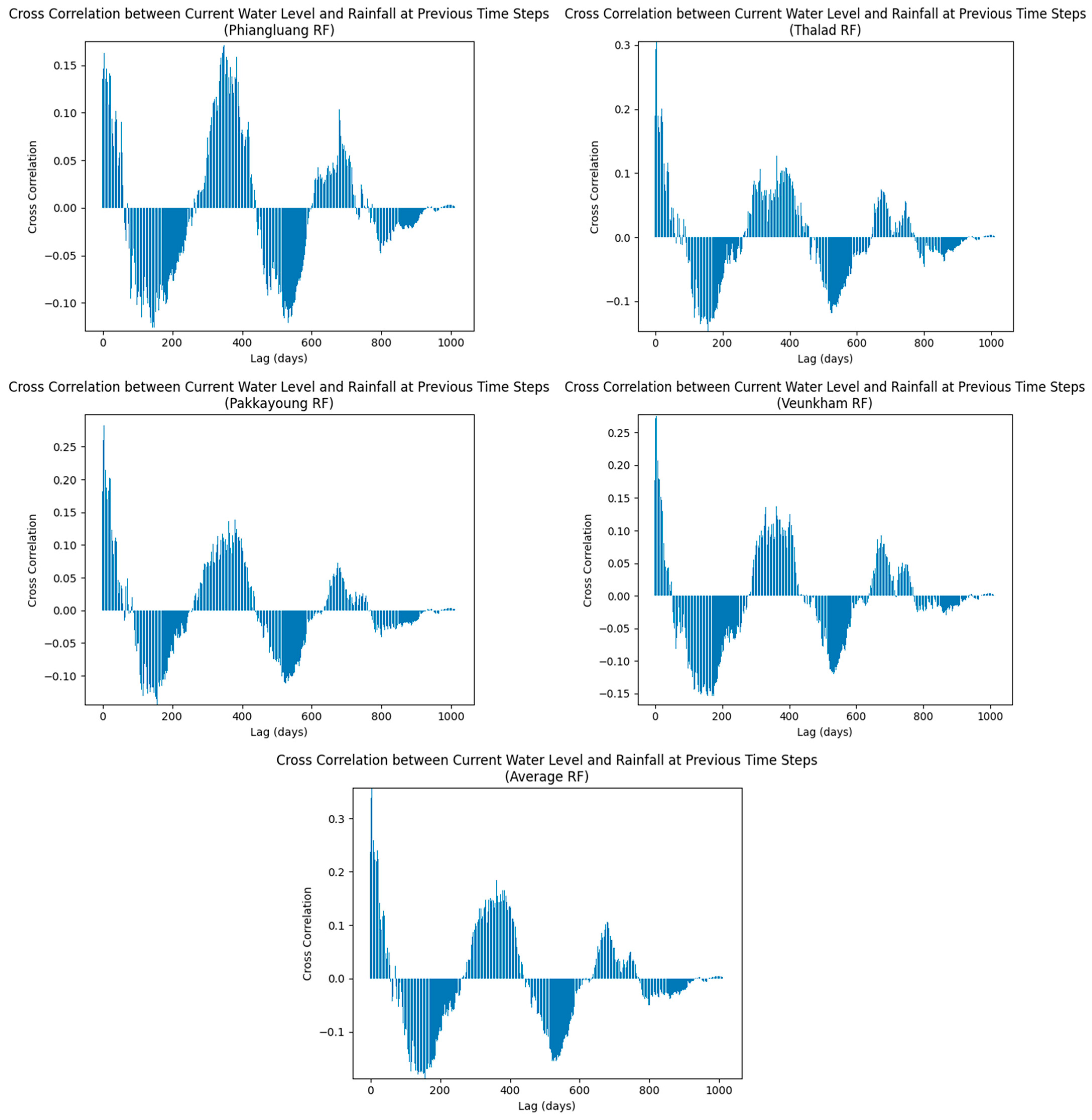
Concentration time is a widely utilized concept in hydrological modeling to characterize the temporal delay between rainfall events and the corresponding runoff response within a watershed. Traditionally, it has been estimated using empirical formulas such as the Kirpich method, which relies on the watershed’s physical characteristics. However, with the advancement of data-driven modeling approaches, the underlying relationship between rainfall and observed streamflow or river water level can now be examined through statistical methods such as cross-correlation analysis.

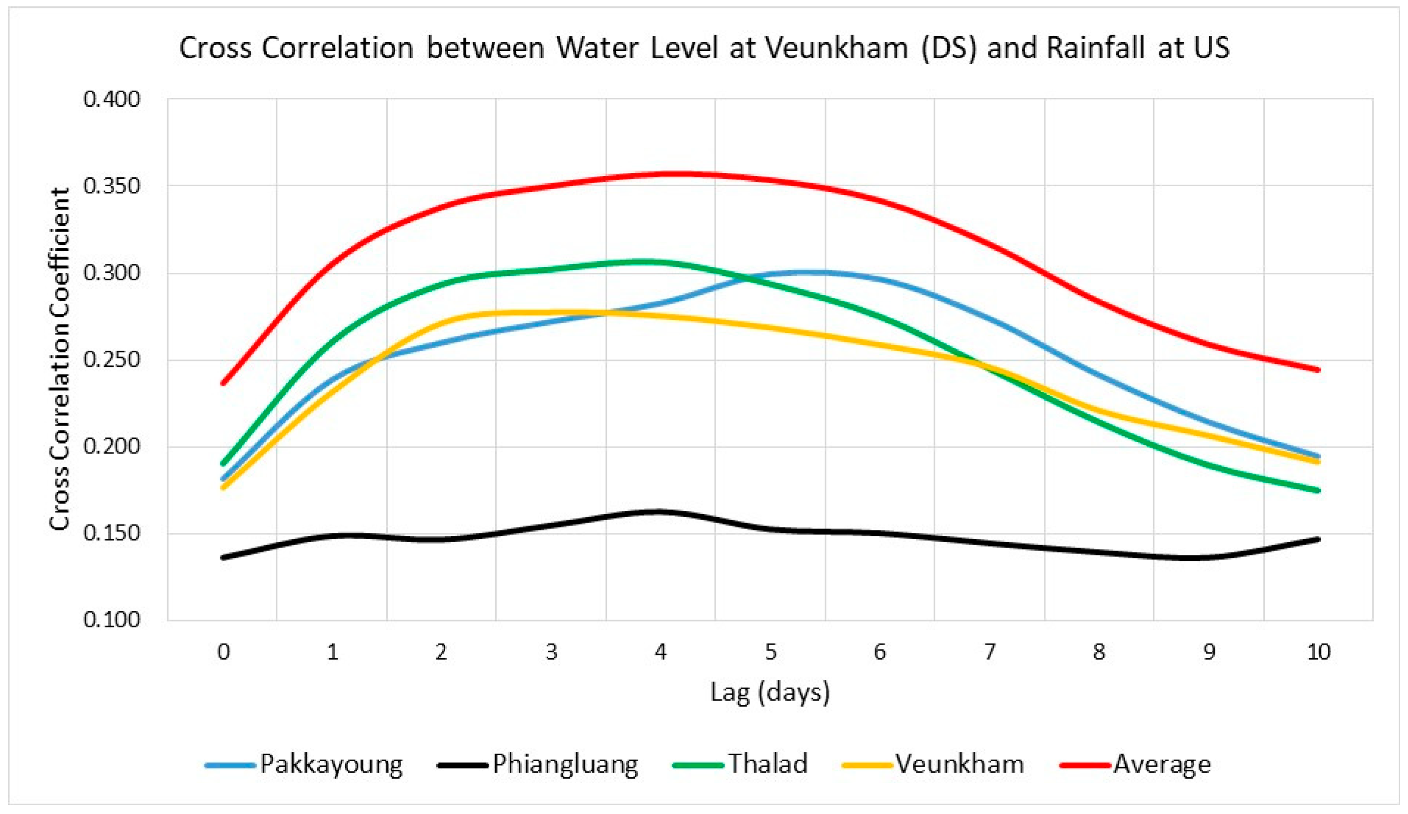
Figure 3 presents the cross-correlation coefficients calculated between water level and both point and average rainfall. A comparison of results between point rainfall and average rainfall (up to 10 lag times) is also presented in Figure 4. The Pakkayoung station exhibited a maximum cross-correlation coefficient of 0.299 at a lag of 5 days. Similarly, the Phiangluang and Thalad stations reached their highest coefficients of 0.163 and 0.306 at a lag of 4 days, respectively, while the Veunkham station showed a peak coefficient of 0.278 at a 3-day lag. Osman et al. [18] mentioned that a positive cross-correlation between rainfall and streamflow or water level with a lag indicates the presence of an autoregressive process. Furthermore, Wei et al. [19] classified correlation coefficients between 0.4 and 0.6 as representing a ‘Medium’ degree of correlation, whereas coefficients ranging from 0.2 to 0.4 correspond to a ‘Weak’ correlation.

It can be observed from Figure 4 that the point rainfall recorded at Phiangluang station exhibited the lowest cross-correlation with the water level observed at Veunkham station. This may be attributed to the geographical locations of the stations: Phiangluang station is situated at the most upstream part of the Ngam Ngum River, whereas Veunkham station is located at the most downstream part, as shown in Figure 1. Additionally, the cross-correlogram for Phiangluang station indicates that its cross-correlation coefficient peaked again after a lag of over 300 days. It is unusual for rainfall events occurring more than 300 days earlier to exert an influence on the water level observed at the current time step. This anomaly further supports that point rainfall recorded at Phiangluang station cannot serve as a reliable precursor for the water level observed at Veunkham station.

The cross-correlation coefficients for point rainfall recorded at Thalad, Pakkayoung, and Veunkham stations were similar, likely due to the proximity of these stations to one another. Interestingly, the average rainfall calculated from the point rainfall data at Phiangluang, Thalad, Pakkayoung, and Veunkham stations yielded the highest cross-correlation with the water level at Veunkham station (represented by the red line in Figure 4, with a maximum coefficient of 0.357 after 4 days of lag). This may inform that point rainfall is insufficient in covering the entire Ngam Ngum watershed due to its limited spatial coverage. Thus, this finding suggests that average rainfall should be used as the input feature, rather than point rainfall recorded at individual stations, to predict the water level at Veunkham station. This is supported by the high cross-correlation observed.

Table 6. Confidence intervals of cross-correlation coefficients.

Rainfall Input	Cross-Correlation Coefficient	Critical Threshold at 95% C.I	Remarks
Phiangluang (Point RF)	0.163 (4 days)	0.062	Significant
Thalad (Point RF)	0.306 (4 days)	0.062	Significant
Pakkayoung (Point RF)	0.299 (5 days)	0.062	Significant
Veunkham (Point RF)	0.278 (3 days)	0.062	Significant
Average RF	0.357 (4 days)	0.062	Significant
Average RF	0.244 (10 days)	0.062	Significant

summarizes the confidence intervals of the cross-correlation coefficients calculated between the point rainfall at each station and the average rainfall against the target water level variable. The numbers in parentheses indicate the lag days corresponding to each cross-correlation coefficient. The results show that all computed cross-correlation coefficients exceeded the critical threshold for the 95% confidence interval, indicating that they are statistically significant. In other words, the likelihood that these observed correlations occurred by random chance under the null hypothesis of no correlation is less than 5%. This suggests that rainfall, particularly average rainfall, was significantly correlated with the target water level variable at the given lag times. These findings further support the appropriateness of using rainfall inputs, especially average rainfall, as predictive features for water level forecasting.

4.2. Optimization of LSTM Water Level Forecasting Model

A default set of hyper-parameters, as presented in

Table 7. Default set of hyper-parameters and performance metrics of baseline simulation.

Baseline Simulation	Neuron Units	Learning Rate		Dropout Rate	Epochs Number		Batch Size
Defaults	32	0.100		0.4	20		32
	Training			Testing			Time Required
	RMSE	NSE	MAE	RMSE	NSE	MAE	(hh:mm:ss)
Baseline Results	1.475	0.202	1.172	1.130	0.065	0.818	0:00:31

, was adopted to implement the LSTM water level forecasting model at the target station. The simulated results obtained using these default hyper-parameters were compared with the observed data, as illustrated in Figure 5. The corresponding performance metrics are also summarized in Table 7. These baseline results serve as a reference for evaluating the effectiveness of the optimization algorithms employed to enhance the LSTM model’s predictive performance, as discussed in subsequent sections.

A total of 24,500 hyper-parameters combinations (5 × 4 × 49 × 5 × 5) were generated based on the search ranges outlined in Table 5 for implementation in a Grid Search approach. Specifically, the search space comprised five values [10, 30, 50, 70, 90] for the number of neurons, four values [0.1, 0.2, 0.3, 0.4] for the dropout rate, forty-nine values (ranging from 0.1 to 0.001 with a step size of 0.002) for the learning rate, five values [16, 32, 48, 64, 80] for the batch size, and five values [10, 30, 50, 70, 90] for the number of epochs.

In contrast, for Random Search and Bayesian Optimization, three experimental scenarios were defined to identify optimal hyper-parameters configurations, consisting of 10, 50, and 100 iterations, respectively. That is, in the scenario with 10 iterations, 10 hyper-parameters combinations were sampled, and the optimal configuration was selected from among these. The final optimized hyper-parameters combinations are presented in

Table 8. Optimal combinations of hyper-parameters identified from respective optimization algorithm.

Optimization Algorithms	Neuron Units	Learning Rate	Dropout Rate	Epochs Number	Batch Size
Grid Search	50	0.095	0.2	10	48
Random Search (10 iterations)	10	0.019	0.4	10	64
Random Search (50 iterations)	90	0.075	0.4	10	80
Random Search (100 iterations)	90	0.095	0.4	50	32
Bayesian Search (10 iterations)	70	0.095	0.2	90	64
Bayesian Search (50 iterations)	90	0.091	0.2	50	80
Bayesian Search (100 iterations)	90	0.091	0.3	70	64

and the optimization results are summarized in

Table 9. The performance of the LSTM model based on the optimal combinations of hyper-parameters identified from respective optimization algorithm.

Optimization Algorithms	Training			Testing			Time Required (hh:mm:ss)
	RMSE	NSE	MAE	RMSE	NSE	MAE
Grid Search	1.494	0.180	1.153	1.157	0.020	0.890	24:22:19
Random Search (10 iterations)	1.408	0.273	1.116	1.014	0.247	0.831	0:00:43
Random Search (50 iterations)	1.528	0.143	1.182	1.120	0.082	0.901	0:05:39
Random Search (100 iterations)	1.621	0.035	1.264	1.098	0.117	0.837	0:12:13
Bayesian Search (10 iterations)	1.435	0.244	1.133	0.990	0.283	0.782	0:02:16
Bayesian Search (50 iterations)	1.425	0.254	1.125	1.017	0.242	0.803	0:10:12
Bayesian Search (100 iterations)	1.429	0.251	1.129	1.034	0.217	0.817	0:20:50

.

It can be seen from Table 9 that Grid Search yielded the least promising results compared to the others; generally, Grid Search performs worse than Random and Bayesian Search for several reasons, particularly in high-dimensional parameter spaces or when dealing with complex models. We all know that Grid Search evaluates every possible combination of parameters in a predefined grid. As the number of parameters (dimensions) increases, the number of combinations grows exponentially. It can be observed in Table 9 that around 24 h searching time was required for Grid Search to identify the optimal combinations of hyper-parameters in this study. In contrast, only several minutes were required for Random and Bayesian Search to identify the optimal combinations of hyper-parameters, and their performances were far better than Grid Search. This elucidates that Grid Search was not only ineffective in terms of computational time, but also wasted computational resources in evaluating poor parameter combinations, as it explored the parameter space uniformly, regardless of whether certain regions were more promising than others. Apart from that, Grid Search also suffers from a lack of adaptation ability, where it does not adapt its search strategy based on previous results, resulting in it evaluating all points in the grids regardless of whether some regions are clearly suboptimal. This will be eventually followed by the problem of overfitting to the grid as it is limited by the granularity of the grid; if the grid is too coarse, it may miss the optimal parameter values. Inversely, if the grid is too fine, it becomes computationally prohibitive. These factors may explain why the Grid Search algorithm in this study performed poorly in identifying optimal hyper-parameter combinations for predicting and forecasting river water levels.

In Random Search, the results obtained indicate that having more iterations does not always improve the performance of optimized hyper-parameters due to several reasons. It may be a result of the random nature of this searching algorithm. Random Search randomly samples parameter combinations from a defined space; it does not guarantee better results with more iterations, as it may not explore the most promising regions of the parameter space effectively. Secondly, Random Search can quickly find optimum parameter combinations initially, but as it continues, the likelihood of finding significantly better combinations decreases, leading to diminishing returns where additional iterations provide minimal or no improvement. Apart from that, in high dimensional parameter spaces, the search spaces become vast enough that the random sampling may miss the optimal regions. Consequently, more iterations do not necessarily ensure better coverage, as Random Search lacks a mechanism to focus on the optimal regions. Lastly, unlike other advanced optimization techniques like Bayesian optimization, Random Search does not learn from previous iterations. Since it does not use past results to guide future sampling, it may repeatedly sample suboptimal regions.

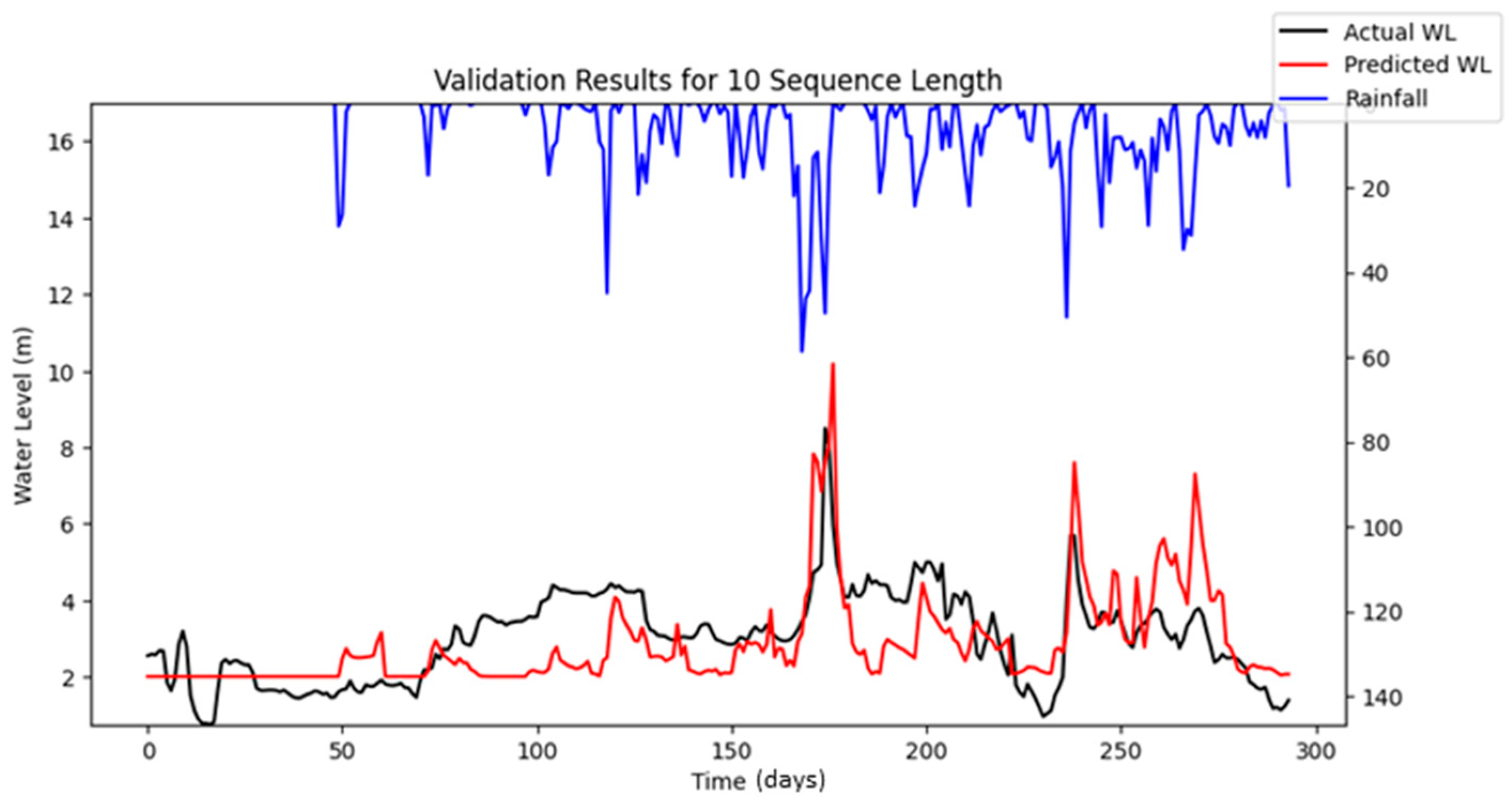
Bayesian Search uses a surrogate model (Gaussian processes) to approximate the objective function and an acquisition function to decide where to sample the future combinations. This allows it to balance exploration (searching new regions) and exploitation (focusing on promising regions). It is less affected by the curse of dimensionality, as it does not rely on fixed grid structure, allowing it to explore the parameter space more flexibly and making it highly adaptive to predict promising regions and focus the searches there. As a result, Bayesian Search often finds better solutions and outperforms Grid and Random Search. The optimization results showed that Random Search performance fluctuated across iterations, whereas Bayesian Search remained relatively stable. Furthermore, both RMSE and MAE metrics indicated that Bayesian Search achieved lower error values relative to the other optimization methods evaluated. However, similar to Random Search, the performance of Bayesian Search did not improve significantly as well with an increasing number of iterations. However, both Random Search and Bayesian Optimization led to improvements in forecasting accuracy compared to the baseline simulation. Notably, the Nash–Sutcliffe Efficiency (NSE) values achieved through these optimization methods were significantly higher, particularly during the testing period. This indicates that the optimized models demonstrated consistently strong performance across both the training and testing phases. The visualizations of simulated water level versus observed water level in training and testing periods using optimal combinations of hyper-parameters identified from respective searching algorithms are portrayed in Figure 6, Figure 7, Figure 8, Figure 9, Figure 10, Figure 11 and Figure 12.

Based on the optimization results concluded from this study, the performances of respective optimization or searching algorithm can be summarized according to particular criteria depicted in

Table 10. Summary of functionality of respective optimization algorithms.

Criteria	Grid Search	Random Search	Bayesian Search
Efficiency	Exhaustive, slow	Faster, broad search	Smart, adaptive search
Coverage	Omits or misses between grid points	Covers broad space better	Focuses on promising regions
Curse of Dimensionality	Yes	Less severe	Handles well
Computational Cost	Very high	Low to Moderate	Low to Moderate
Adaptability	No	Partially	Yes (Able to learn from past)

. Grid Search is time-exhaustive, has slow efficiency, and may also miss optimal solutions located in between the grid points. Apart from that, it suffers from the curse of dimensionality and requires a very high computational cost. Lastly, it has no adaptability during its searching process by learning from the previous search.

4.3. Reproducible LSTM Simulations

The optimized LSTM simulations, as discussed in previous sections, are all based on stochastic simulations where the simulated results are not reproducible, as the results will be different in each simulation due to the random nature of LSTM model. This random nature may introduce problems for flood forecasting in the real world, as different forecasting results will be obtained in each simulation even though identical inputs are fed into the trained and optimized LSTM model. To resolve this, the architecture of the LSTM model has been modified to ensure the reproducibility of the forecasted results by defining a constant random seed of 42 for any random modules adopted in the LSTM model. Apart from that, the environment variables used in Tensorflow 2.15.0 have also been enforced to follow deterministic operations, which ensures that the computations using Tensorflow 2.15.0 in the LSTM model will produce the same results every time when identical inputs are fed into the model, which is useful for reproducibility of the prediction of water level for flood forecasting.

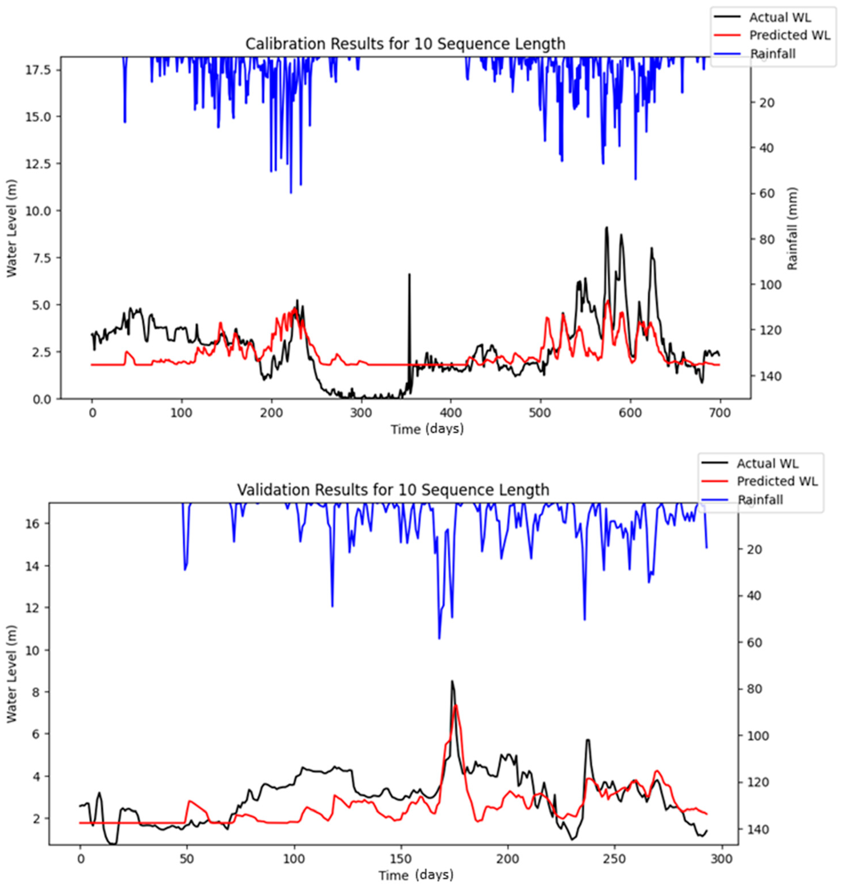
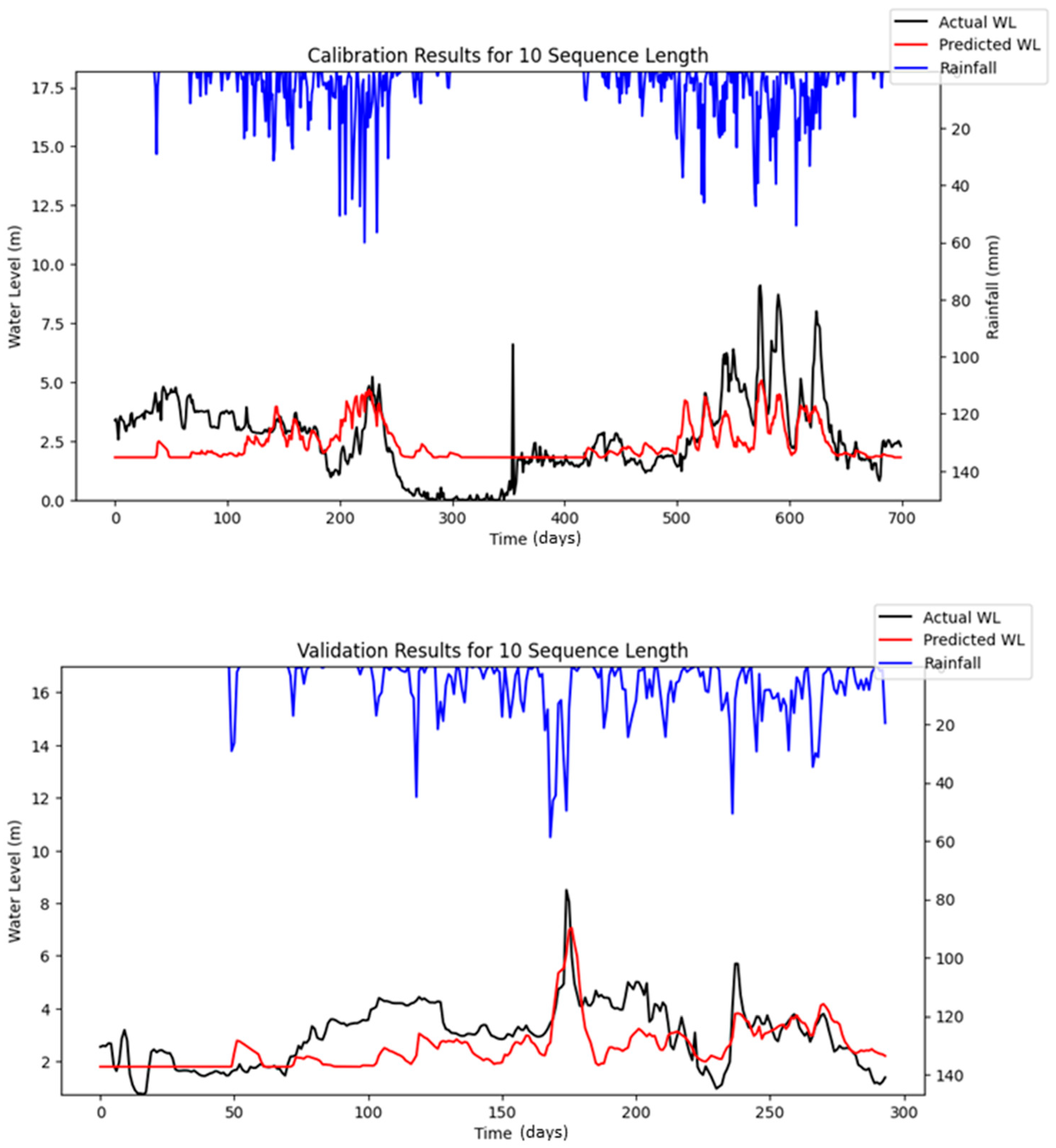
The optimization using Bayesian Search was re-conducted by using the modified LSTM model to allow for reproducible simulation; the optimized results and their performances are depicted in

Table 11. Optimal combinations of hyper-parameters identified from Bayesian Search using reproducible LSTM simulation.

Optimization Algorithms	Neuron Units	Learning Rate	Dropout Rate	Epochs Number	Batch Size
Bayesian Search (10 iterations)	63	0.042	0.244	80	65
Bayesian Search (50 iterations)	22	0.00068	0.438	35	92
Bayesian Search (100 iterations)	22	0.00063	0.499	39	96

and

Table 12. The performance and time efficiency of the optimal combinations of hyper-parameters identified from Bayesian Search using reproducible LSTM simulation.

Optimization Algorithms	Training			Testing			Time Required (hh:mm:ss)
	RMSE	NSE	MAE	RMSE	NSE	MAE
Bayesian Search (10 iterations)	1.159	0.507	0.923	1.128	0.068	0.909	0:02:32
Bayesian Search (50 iterations)	1.409	0.271	1.102	1.085	0.138	0.863	0:08:36
Bayesian Search (100 iterations)	1.411	0.269	1.105	1.076	0.152	0.857	0:18:34

. The simulated results for respective iterations are portrayed in Figure 13, Figure 14 and Figure 15.

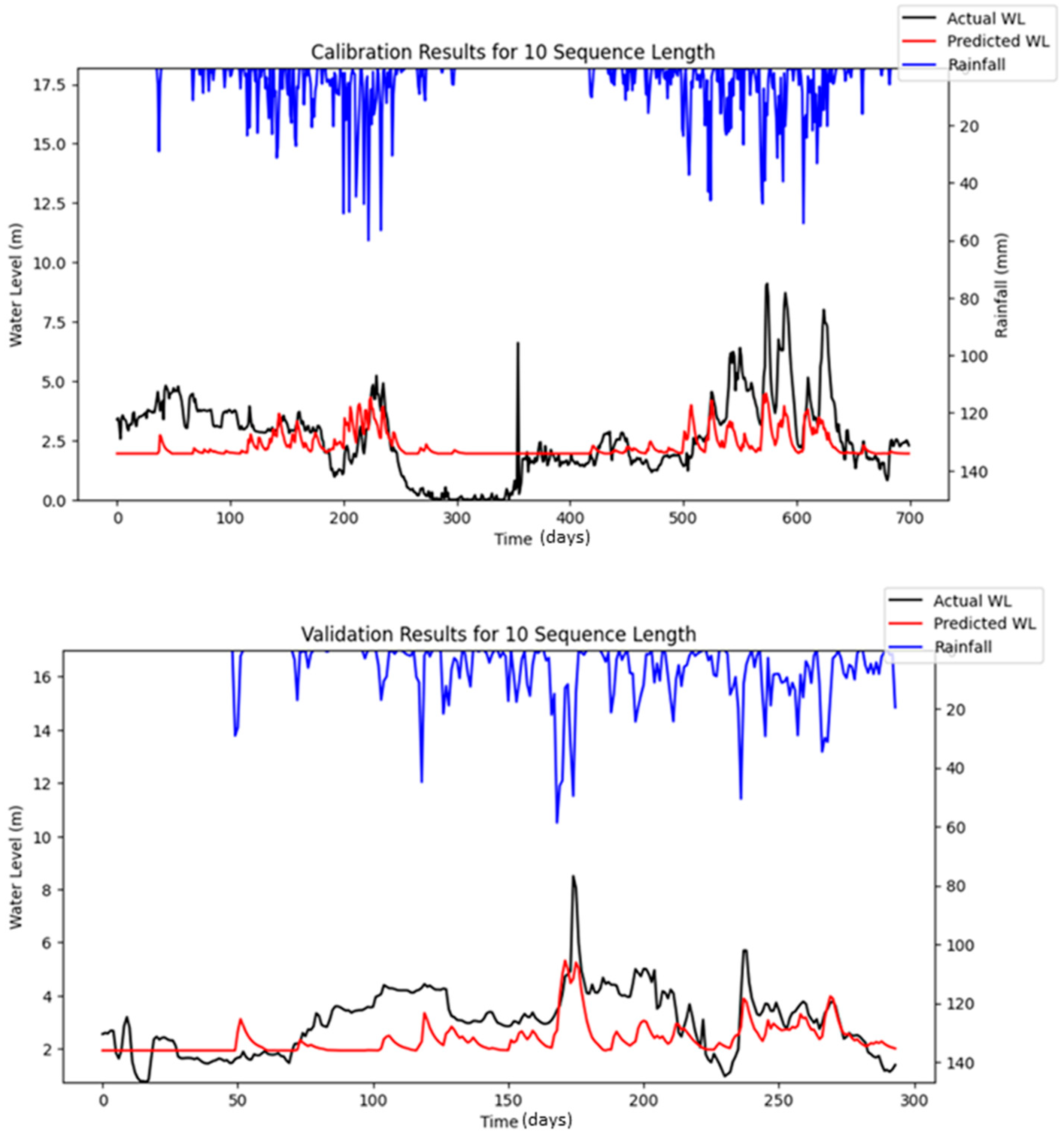
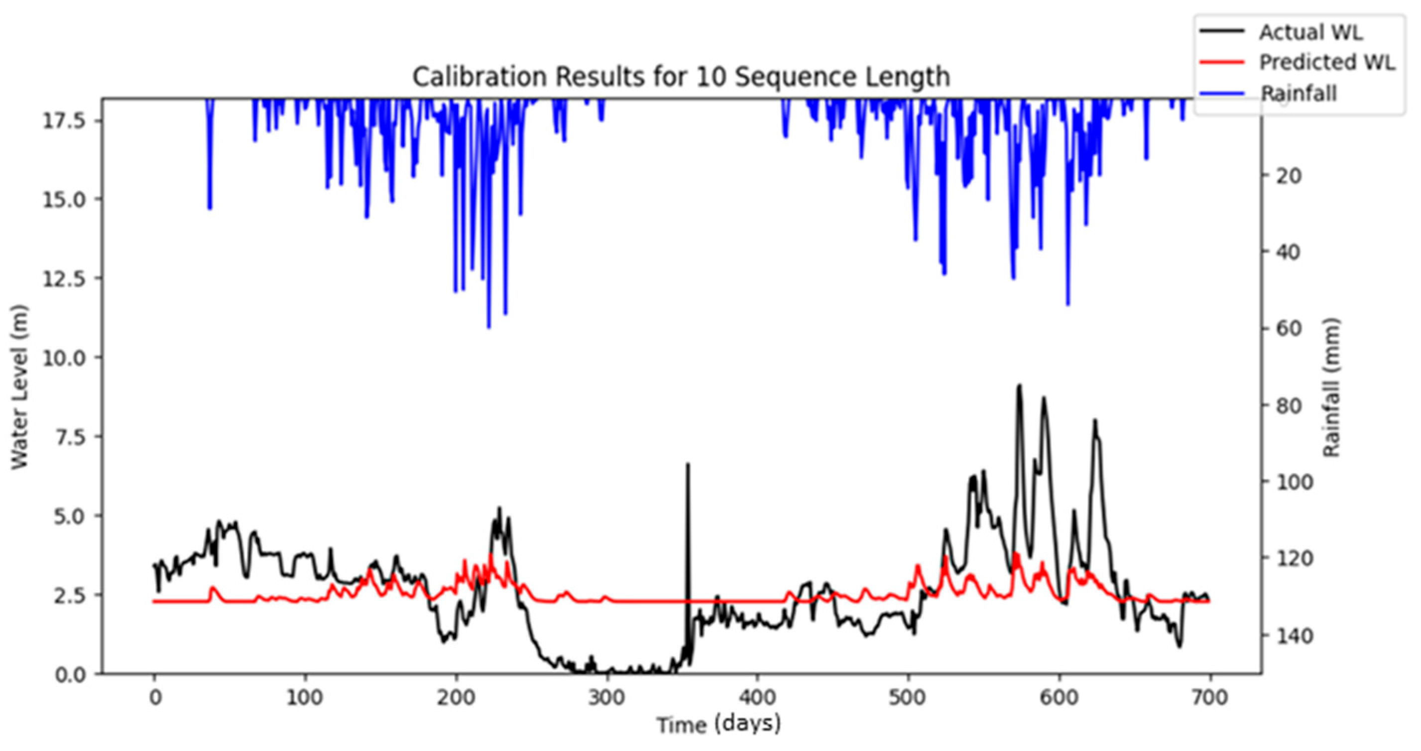
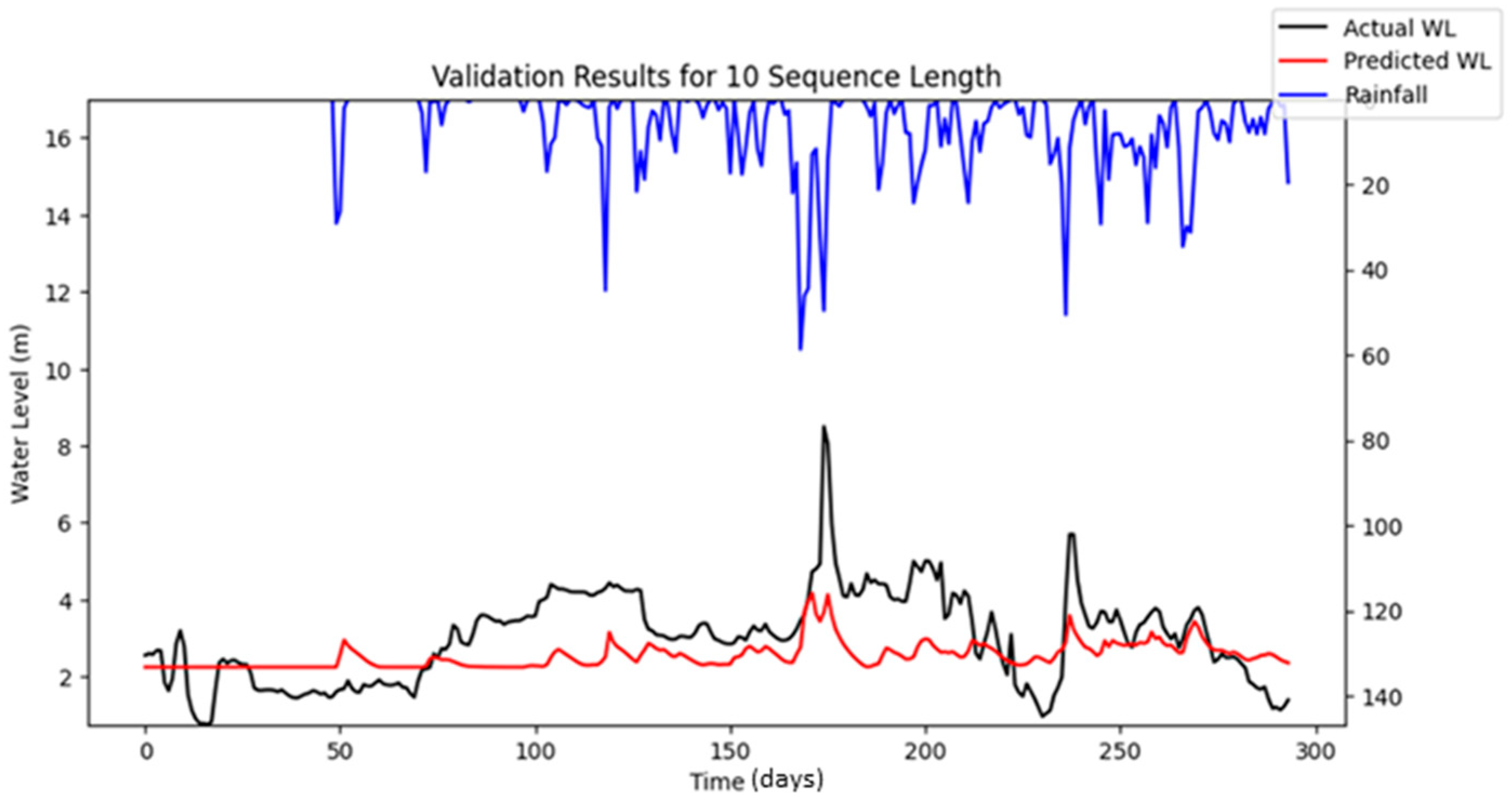
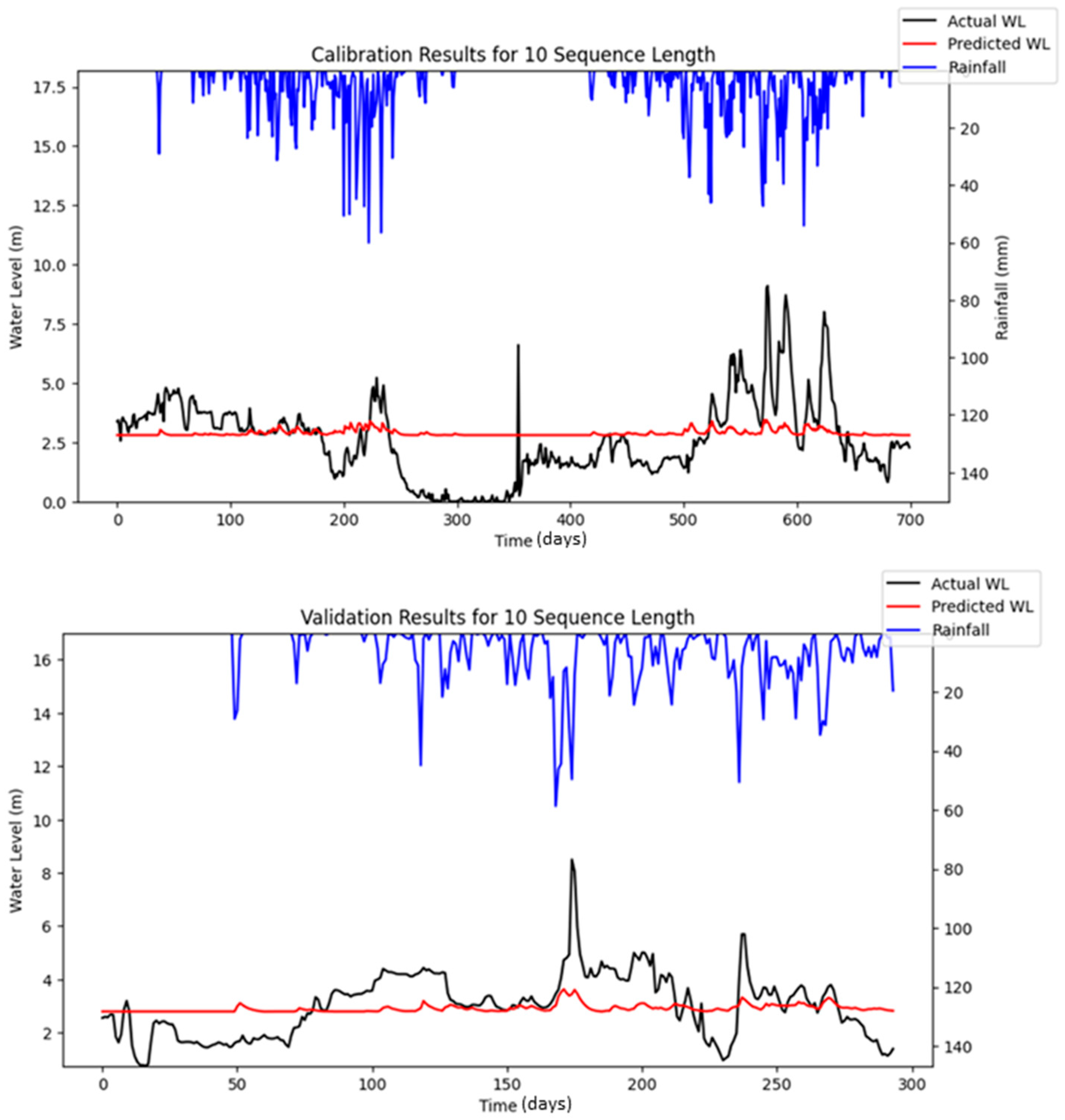
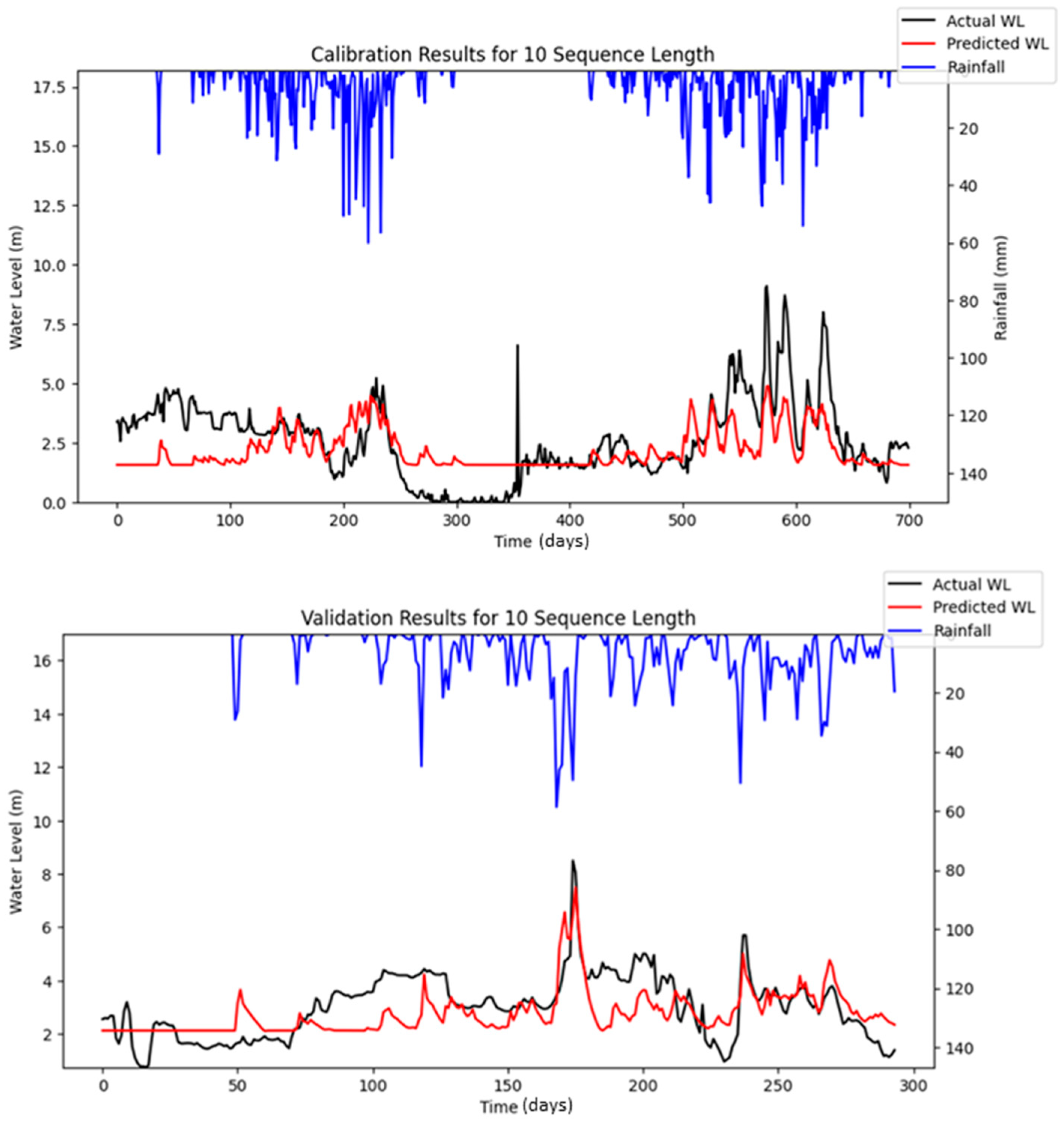
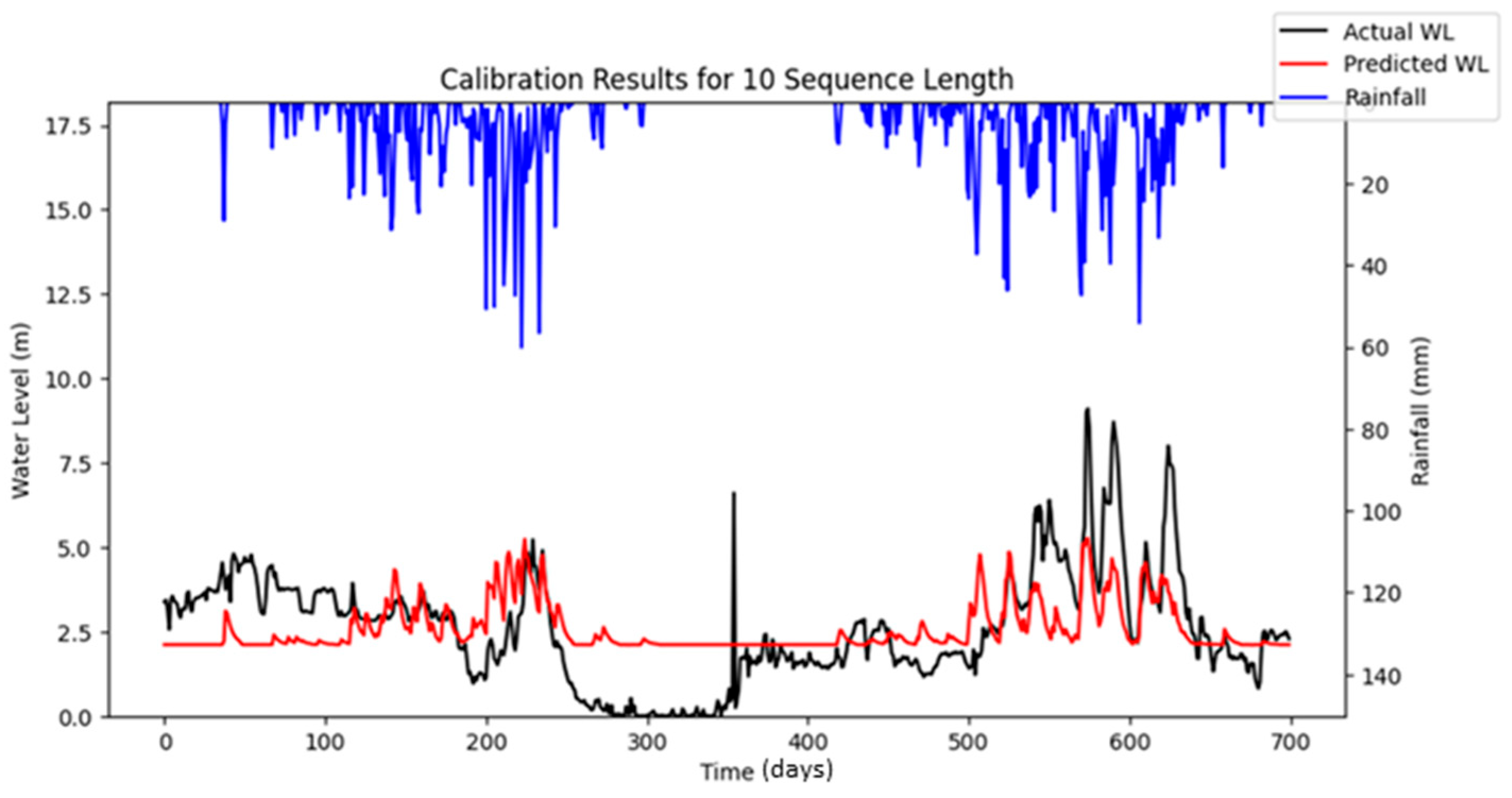
The Nash–Sutcliffe Efficiency (NSE) quantifies the degree to which model predictions correspond to observed values relative to the predictive accuracy achieved by using the mean of the observed data as a benchmark. The optimization results obtained from Bayesian Search using reproducible LSTM simulations indicate that the reproducible LSTM model performed slightly better than simply predicting the mean water level, as an average NSE of about 0.100 was obtained in the testing period during the specified iterations. The optimized models performed better in the training period than in the testing period, where an NSE as high as 0.507 was achieved during the optimization of 10 iterations. However, the results of RMSE indicated that the model’s predictions in the testing period had fewer errors than in the training period. The model’s predictions deviated from the actual water level by about 0.89 m on average (MAE = 0.089), and the typical magnitude of error was around 1.128 m (RMSE = 1.128) in the testing period. This was relatively close to the training RMSE and MAE of 1.159 and 0.916, respectively, which suggests that the model generalized similarly on both the training and test sets, but it might still indicate that the model could improve its accuracy. It is important to note that, while reproducible simulations can yield consistent results for real-world flood forecasting, they do not necessarily guarantee superior performance compared to stochastic simulation approaches.

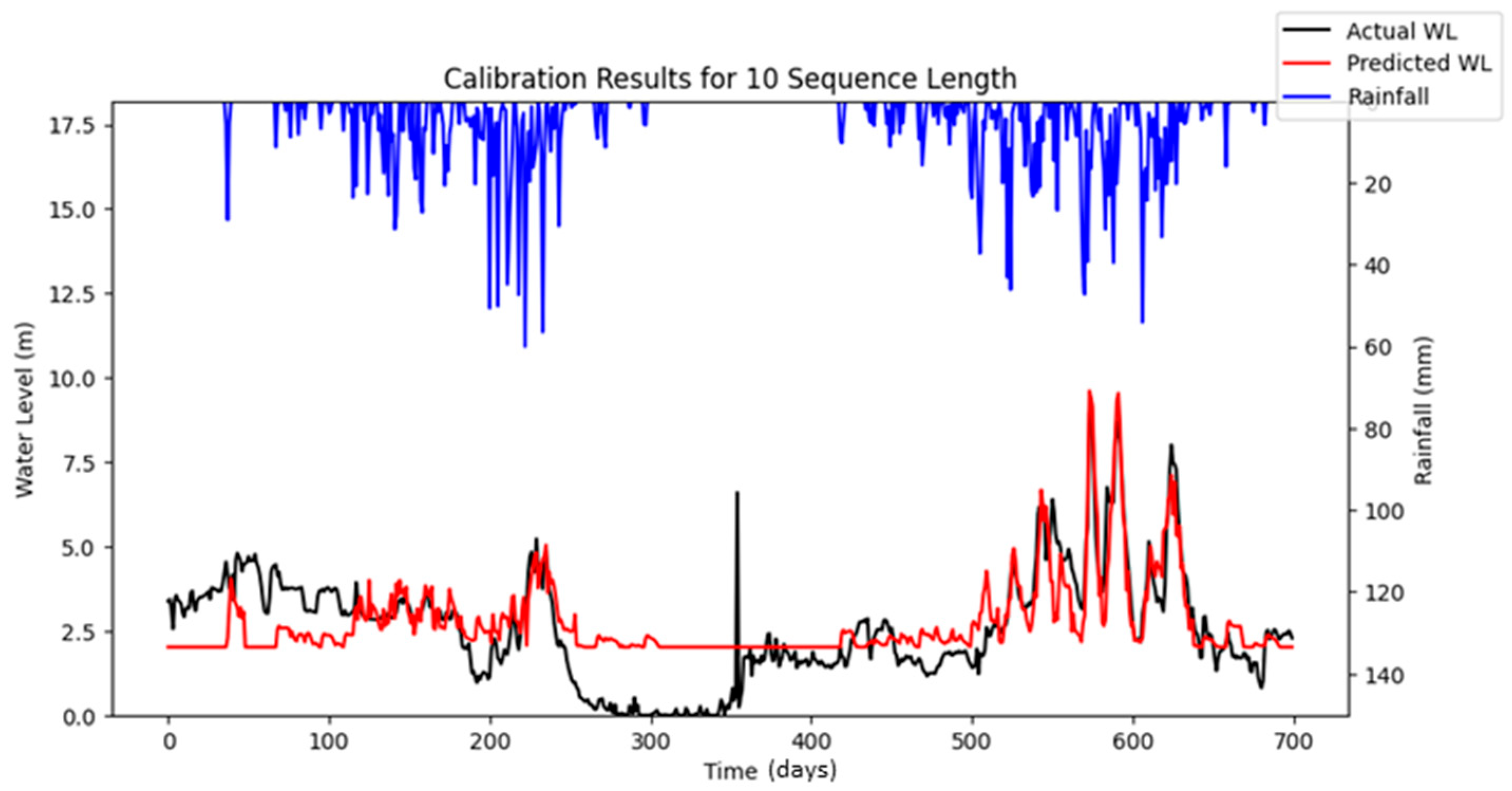
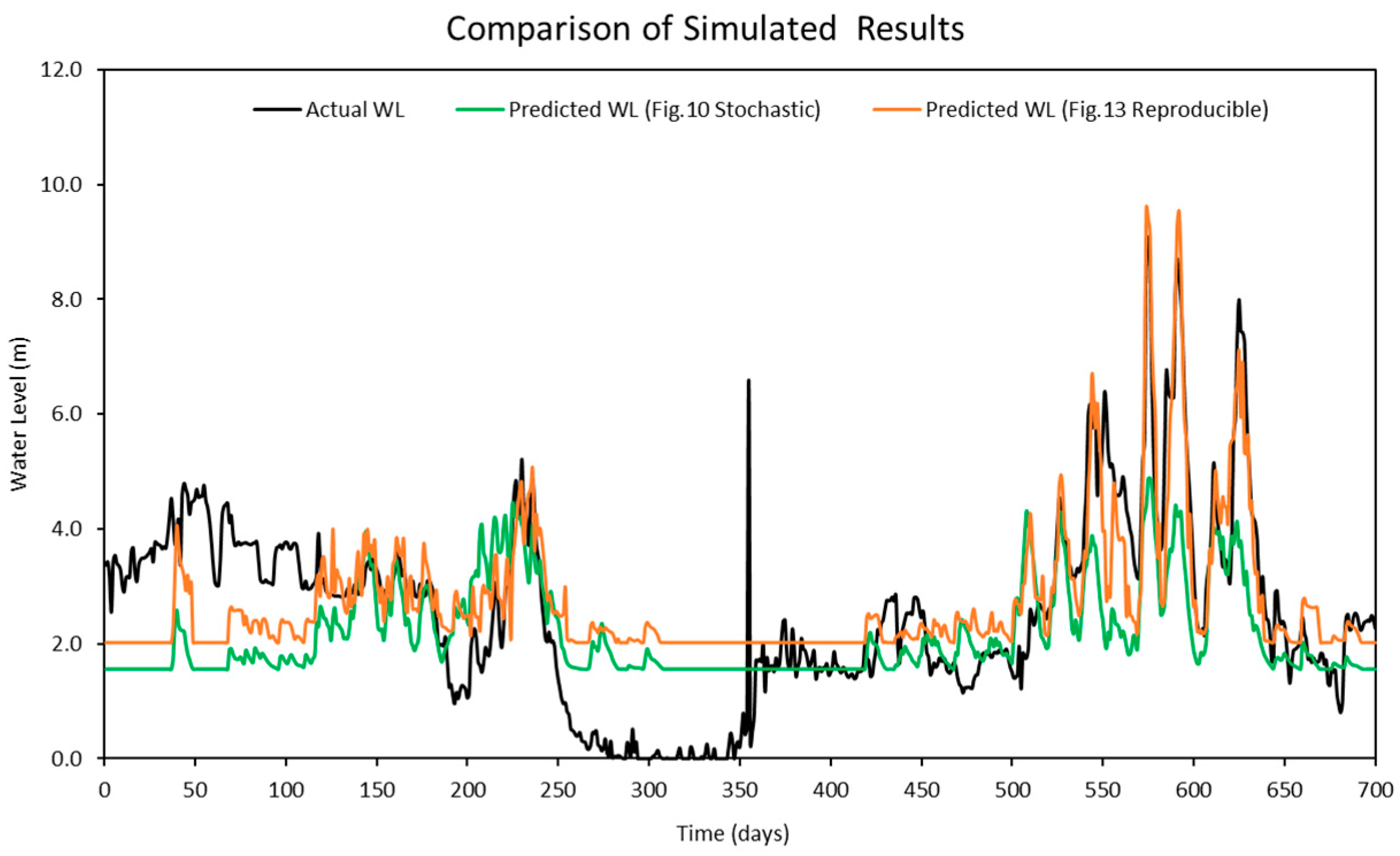
Figure 16 highlights the differences between the stochastic simulation shown in Figure 10 and the reproducible simulation presented in Figure 13 during the calibration period for 10 iterations. The comparison reveals that the results from the reproducible simulation (Figure 13) demonstrated better performance than those from the stochastic simulation (Figure 10). The improved prediction performance observed in Figure 13 is likely due to the more suitable set of hyper-parameters being identified during the optimization process in reproducible simulation, which resulted in a better model fit compared to the predictions in Figure 10 for the calibration.

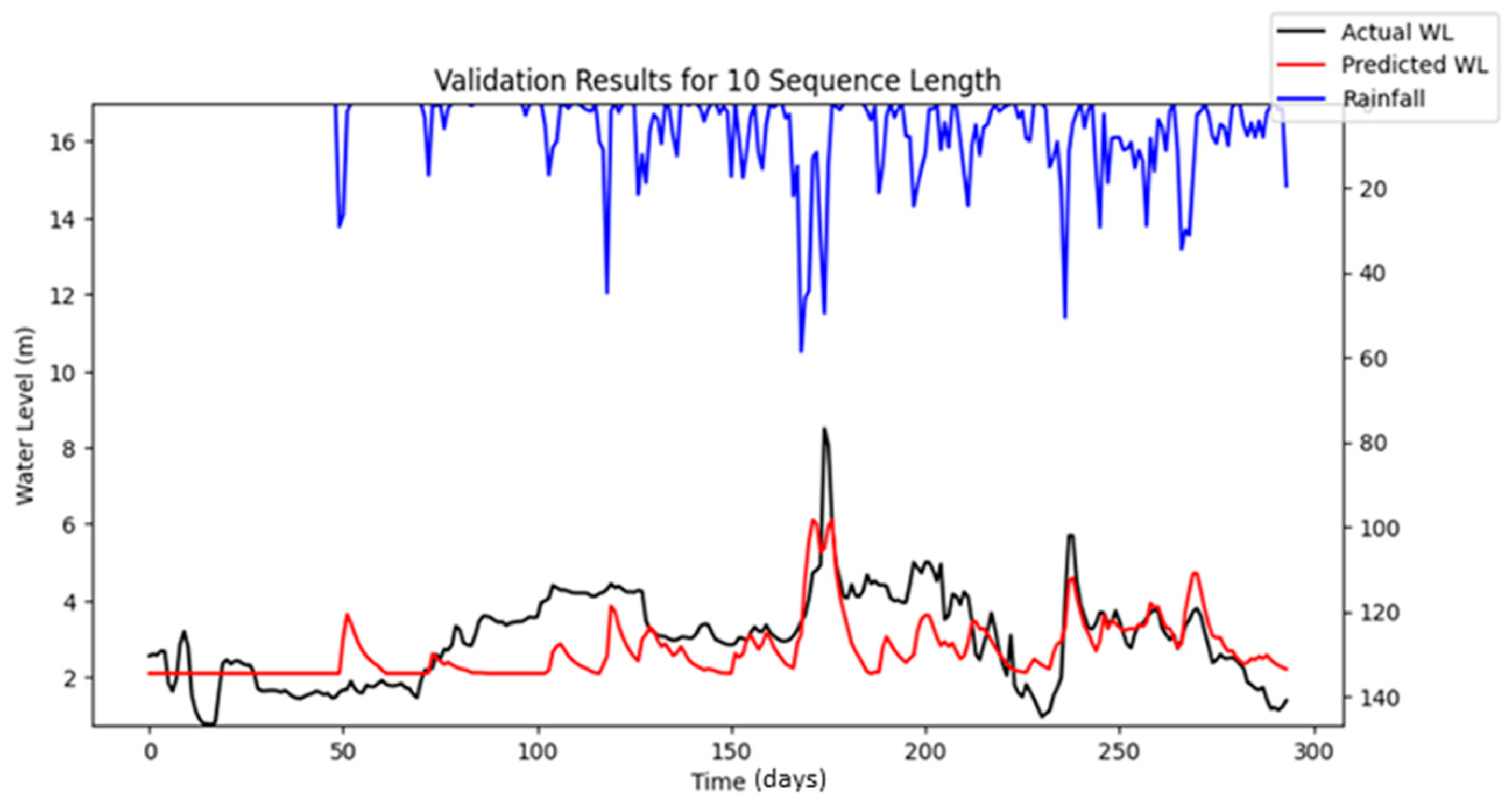
Another notable finding is that the prediction accuracy during calibration appeared to decrease over iterations, whereas no significant fluctuations were observed in the validation results. This may be attributed to differences in the data period length and the occurrence of peak events within the respective datasets. Specifically, the calibration period spanned a longer timeframe and encompassed a wider range of hydrological conditions, including more frequent or extreme peak flow events. These events are often more challenging for the model to accurately learn and predict, particularly when input features do not fully capture the factors driving such variability (e.g., dam releases or sudden rainfall bursts). In contrast, the validation period was shorter and included fewer or less intense peak events, resulting in more stable and consistent prediction performance during validation.

To improve the prediction accuracy of water levels using the LSTM model, it is necessary to increase the diversity of input features used for training. Currently, only the average daily rainfall from upstream stations was used as an input. As a result, the average daily rainfall is believed to have a direct impact only on the predicted water levels during rising limbs or peak periods. The relationship between average daily rainfall and predicted water levels during falling limbs, especially during plunges, is likely minimal. This is evident in the simulation results, where the predicted water levels closely aligned with the observed values during storm events but deviated significantly when the water levels were at their lowest.

We recognize that the issue discussed in the previous paragraph may be influenced by the presence of dams located upstream of the stations studied. The unusually low water levels recorded at the stations could be the result of restricted dam releases, which were implemented to secure additional water storage for meeting domestic and agricultural demands during drought conditions. Unfortunately, the dam release data from these upstream dams could not be obtained and were therefore not included as inputs for this study. It is believed that incorporating dam release data into the LSTM model would significantly improve the accuracy of water level predictions, particularly during periods of low water levels. We will actively seek solutions to gain access to this data and aim to address the issue in future studies as soon as possible.

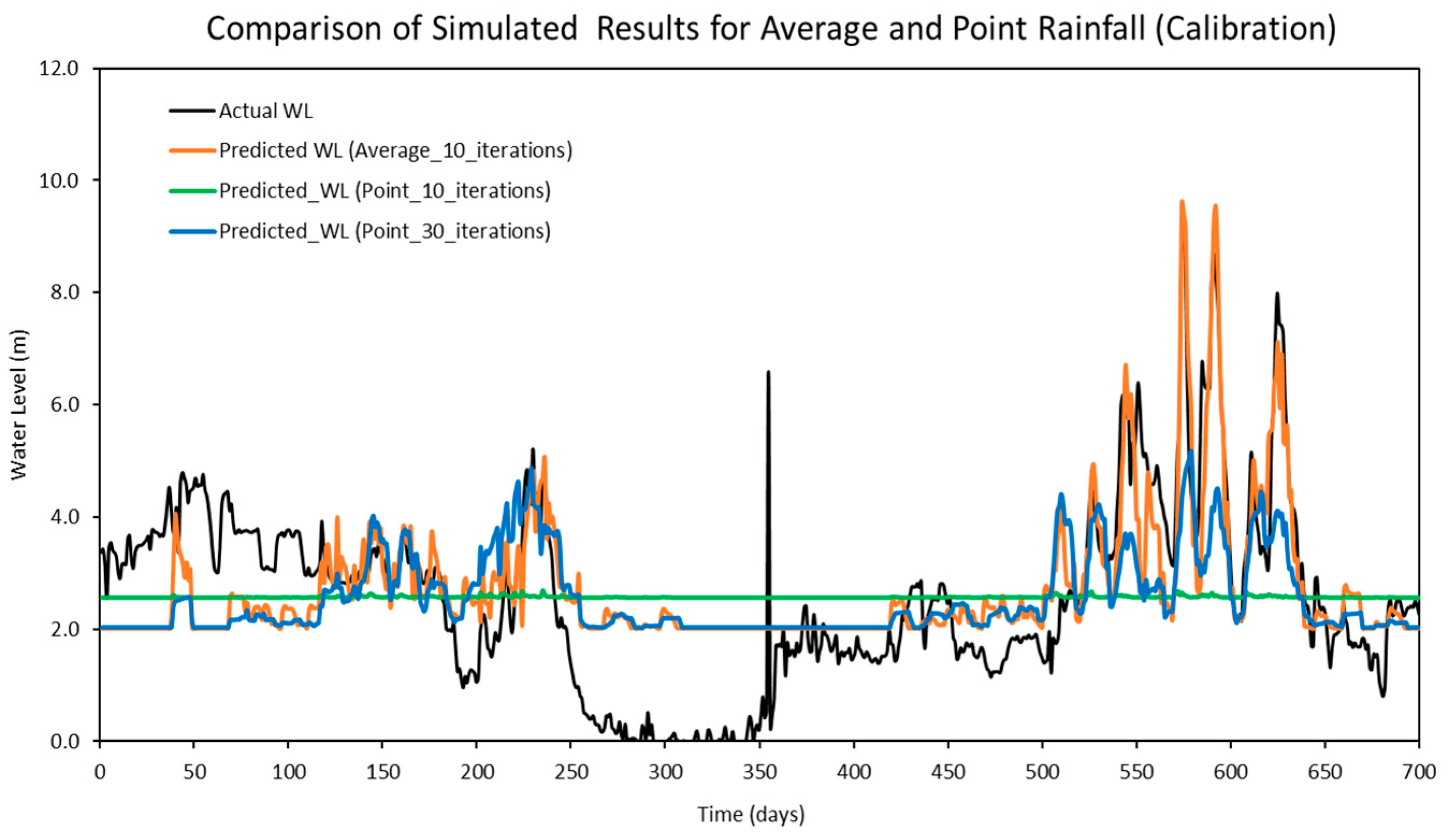
Another comparison was conducted to evaluate the model’s performance using two different input configurations in reproducible simulations: point rainfall collected from four individual stations and average rainfall.

Table 13. Optimal combinations of hyper-parameters identified from Bayesian Search using point rainfall inputs.

Optimization Algorithms	Neuron Units	Learning Rate	Dropout Rate	Epochs Number	Batch Size
Bayesian Search (10 iterations)	88	0.071	0.221	89	83
Bayesian Search (30 iterations)	99	0.0001	0.234	18	54

presents the optimized hyper-parameters derived from the point rainfall input, while the performance metrics for both configurations are summarized in

Table 14. The performance and time efficiency of the optimal combinations of hyper-parameters identified from Bayesian Search using point rainfall and average rainfall inputs.

Optimization Algorithms	Iterations	Training			Testing			Time Required (hh:mm:ss)
		RMSE	NSE	MAE	RMSE	NSE	MAE
Bayesian Search (Average RF)	10	1.159	0.507	0.916	1.128	0.068	0.890	0:02:32
Bayesian Search (Point RF)	10	1.644	0.007	1.279	1.236	−0.119	1.007	0:02:32
Bayesian Search (Point RF)	30	1.391	0.289	1.104	1.034	0.216	0.854	0:04:49

. The comparison results indicate that the LSTM model using point rainfall as an input feature required more computational time during the optimization process, as it needed a higher number of iterations to identify the optimal hyper-parameters. Specifically, the optimal configuration could not be achieved within 10 iterations, and noticeable improvements in model performance were only observed when the number of iterations was increased to 30. In contrast, the LSTM model using average rainfall as an input feature was able to reach optimal performance within just 10 iterations. Furthermore, as illustrated in Figure 17, the predicted results based on point rainfall inputs (green and blue lines) were less effective in capturing peak water levels compared to those based on average rainfall (orange line). In particular, the predictions using point rainfall at 10 iterations (green line) exhibited inadequate responsiveness, with the predicted water levels failing to rise in alignment with the observed peaks. These findings suggest that average rainfall can be adopted as a more suitable surrogate input in real-world applications, particularly when working with large datasets or high-dimensional inputs, as it requires a shorter computational time to enhance the predictive accuracy of flood forecasting using a LSTM model.

5. Conclusions

In conclusion, three optimization algorithms, Grid Search, Random Search, and Bayesian Search, were successfully employed to identify the optimal hyper-parameters for predicting and forecasting river water levels at the target station using an LSTM model. The results indicated that, while Grid Search was the most time-consuming, both Random Search and Bayesian Search identified optimal hyper-parameters in significantly less time. The model optimized using Bayesian Search performed slightly better than that optimized using Random Search. Although the performance improvement was not statistically significant, Bayesian Search is recommended for hyper-parameter optimization due to its balanced trade-off between accuracy and time efficiency when forecasting river water levels with LSTM models. Additionally, this study implemented a reproducible LSTM simulation for water level prediction to ensure the consistency and applicability of the forecasted results in real-world scenarios. We acknowledge that there is still room for improving the accuracy of water level predictions, particularly during low water level periods. One potential improvement is increasing the diversity of input features used to train the LSTM model. The issue of unusually low water levels recorded at the stations, potentially caused by restricted dam releases from upstream dams, is expected to be addressed in future studies by obtaining access to dam release data and incorporating it into the LSTM water level forecasting model.

References

1. Guo, Z.; Leitão, J.-P.; Simões, N.-E.; Moosavi, V. Data-driven flood emulation: Speeding up urban prediction by deep convolutional neural network. J. Flood Risk Manag. 2021, 14, e12684. [Google Scholar] [CrossRef]
2. Guglielmo, G.; Montessori, A.; Tucny, J.-M.; La Rocca, M.; Prestininzi, P. A priori physical information to aid generalization capabilities of neural networks for hydraulic modeling. Front. Complex. Syst. 2025, 2, 1508091. [Google Scholar] [CrossRef]
3. Kratzert, F.; Klotz, D.; Herrnegger, M.; Sampson, A.; Hochreiter, S.; Nearing, G. Towards improved predictions in ungauged basins: Exploiting the power of machine learning. Water Resour. Res. 2019, 55, 11344–11354. [Google Scholar] [CrossRef]
4. Xu, Y.; Hu, C.; Wu, Q.; Jian, S.; Li, Z.; Chen, Y.; Zhang, G.; Zhang, Z.; Wang, S. Research on particle swarm optimization in LSTM neural networks for rainfall-runoff simulation. J. Hydrol. 2022, 608, 127553. [Google Scholar] [CrossRef]
5. Janizadeh, S.; Vafakhah, M.; Kapelan, Z.; Dinan, N.M. Hybrid XGboost model with various Bayesian hyperparameter optimization algorithms for flood hazard susceptibility modeling. Geocarto Int. 2022, 37, 8273–8292. [Google Scholar] [CrossRef]
6. Li, W.; Liu, C.; Hu, C.; Niu, C.; Li, R.; Li, M.; Xu, Y.; Tian, L. Application of a hybrid algorithm of LSTM andTransformer based on random search optimization for improving rainfall-runoff simulation. Sci. Rep. 2024, 14, 11184. [Google Scholar] [CrossRef]
7. Ruma, J.F.; Adnan, M.S.G.; Dewan, A.; Rahman, R.M. Particle swarm optimization based LSTM networks for water level forecasting: A case study on Bangladesh river network. Results Eng. 2023, 17, 100951. [Google Scholar] [CrossRef]
8. Li, L.; Jun, K.S. A Hybrid Approach to Improve Flood Forecasting by Combining a Hydrodynamic Flow Model and Artificial Neural Networks. Water 2022, 14, 1393. [Google Scholar] [CrossRef]
9. Aditya, M.; Chandranath, C.; Narendra, S.R. Flood Forecasting Using ANN, Neuro-Fuzzy, and Neuro-GA Models. J. Hydrol. Eng. 2009, 14, 647–652. [Google Scholar]
10. Meema, T.; Tachikawa, Y.; Ichikawa, Y.; Yorozu, K. Uncertainty assessment of water resources and long-term hydropower generation using a large ensemble of future climate projections for the Nam Ngum River in the Mekong Basin. J. Hydrol. Reg. Stud. 2021, 36, 100856. [Google Scholar] [CrossRef]
11. Kim, C.-S.; Kim, C.-R.; Kok, K.-H.; Lee, J.-M. Water Level Prediction and Forecasting Using a LSTM Model for Nam Ngum River Basin in Lao PDR. Water 2024, 16, 1777. [Google Scholar] [CrossRef]
12. Hochreiter, S.; Urgen Schmidhuber, J. Long Short-Term Memory. Neural Comput. 1997, 9, 1735–1780. [Google Scholar] [CrossRef] [PubMed]
13. Kim, D.K.; Kang, S.K. Data collection strategy for building rainfall-runoff LSTM model predicting daily runoff. J. Korea Water Resour. Assoc. 2021, 54, 795–805. [Google Scholar] [CrossRef]
14. Caren, M.; Pavlić, K. Autocorrelation and cross-correlation flow analysis along the confluence of the kupa and sava rivers. Rud. Geol. Naft. Zb. 2021, 36, 67–77. [Google Scholar] [CrossRef]
15. UNCTAD (United Nations Conference on Trade and Development). Handbook of Statistics; United Nations: New York, NY, USA, 2019; ISBN 978-92-1-112940-3. [Google Scholar]
16. Floudas, C.A.; Pardalos, P.M. Encyclopedia of Optimization, 2nd ed.; Springer: Berlin/Heidelberg, Germany, 2009; ISBN 978-0-387-74759-0. [Google Scholar]
17. Caudle, K. Searching Algorithm Using Bayesian Updates. J. Comput. Math. Sci. Teach. 2010, 29, 19–29. [Google Scholar]
18. Osman, Y.; Al-Ansari, N.; Abdellatif, M. Climate change model as a decision support tool for water resources management in northern Iraq: A case study of Greater Zab River. J. Water Clim. Chang. 2019, 10, 197–209. [Google Scholar] [CrossRef]
19. Wei, X.; Zhang, H.; Gong, X.; Wei, X.; Dang, C.; Zhi, T. Intrinsic cross-correlation analysis of hydro-meteorological data in the Loess Plateau, China. Int. J. Environ. Res. Public Health 2020, 17, 2410. [Google Scholar] [CrossRef] [PubMed]
Figure 1. Location of rainfall and water level stations in the Nam Ngum River Basin.
Water 17 02087 g001
Figure 2. Process of locating optimum hyper-parameters using optimization algorithms: (upper left) Grid Search, (upper right) Random Search, (bottom) Bayesian Search.
Water 17 02087 g002
Figure 3. Cross-correlogram between water level and point rainfall at (top left) Phiangluang, (top right) Thalad, (middle left) Pakkayoung, (middle right) Veunkham, and (bottom) average rainfall.
Water 17 02087 g003
Figure 4. Comparison of cross-correlation coefficients computed from between water level at Veunkham and point rainfalls as well as average rainfall.
Water 17 02087 g004
Figure 5. Plots of simulated water level versus observed water level in training (upper) and testing (bottom) periods using a default set of hyper-parameters as baseline simulation.
Water 17 02087 g005
Figure 6. Plots of simulated water level versus observed water level in training (upper) and testing (bottom) periods using optimal combinations of hyper-parameters identified from Grid Search.
Water 17 02087 g006
Figure 7. Plots of simulated water level versus observed water level in training (upper) and testing (bottom) periods using optimal combinations of hyper-parameters identified from Random Search across 10 iterations.
Water 17 02087 g007
Figure 8. Plots of simulated water level versus observed water level in training (upper) and testing (bottom) periods using optimal combinations of hyper-parameters identified from Random Search across 50 iterations.
Water 17 02087 g008aWater 17 02087 g008b
Figure 9. Plots of simulated water level versus observed water level in training (upper) and testing (bottom) periods using optimal combinations of hyper-parameters identified from Random Search across 100 iterations.
Water 17 02087 g009
Figure 10. Plots of simulated water level versus observed water level in training (upper) and testing (bottom) periods using optimal combinations of hyper-parameters identified from Bayesian Search across 10 iterations.
Water 17 02087 g010
Figure 11. Plots of simulated water level versus observed water level in training (upper) and testing (bottom) periods using optimal combinations of hyper-parameters identified from Bayesian Search across 50 iterations.
Water 17 02087 g011aWater 17 02087 g011b
Figure 12. Plots of simulated water level versus observed water level in training (upper) and testing (bottom) periods using optimal combinations of hyper-parameters identified from Bayesian Search across 100 iterations.
Water 17 02087 g012
Figure 13. Plots of simulated water level versus observed water level in training (upper) and testing (bottom) periods using optimal combinations of hyper-parameters identified from Bayesian Search using reproducible LSTM simulation of 10 iterations.
Water 17 02087 g013aWater 17 02087 g013b
Figure 14. Plots of simulated water level versus observed water level in training (upper) and testing (bottom) periods using optimal combinations of hyper-parameters identified from Bayesian Search using reproducible LSTM simulation of 50 iterations.
Water 17 02087 g014
Figure 15. Plots of simulated water level versus observed water level in training (upper) and testing (bottom) periods using optimal combinations of hyper-parameters identified from Bayesian Search using reproducible LSTM simulation of 100 iterations.
Water 17 02087 g015
Figure 16. Comparison of simulated results from stochastic (Figure 10) and reproducible (Figure 13) simulation during the calibration period.
Water 17 02087 g016
Figure 17. Comparison of simulated results from using point and average rainfall inputs during the calibration period.
Water 17 02087 g017