Numerical Models for Predicting Water Flow Characteristics and Optimising a Subsurface Self-Regulating, Low-Energy, Clay-Based Irrigation (SLECI) System in Sandy Loam Soil

Abstract

The Subsurface self-regulating, Low-Energy, Clay-based Irrigation (SLECI) system is a recently developed irrigation method. The SLECI system supplies water directly to the crop root zone by utilising the potential difference established between its permeable interior and exterior radial walls. In this study, we investigated the effect of the SLECI emitter’s operating pressure head and burial depth on the water flow characteristics in sandy loam soil. The results show that the developed COMSOL-2D model accurately predicted water flow characteristic under SLECI. The operating pressure head significantly influenced the water flow characteristics. As the operating pressure head increased, emitter discharge increased, and the wetted soil area was extended. The burial depth had a minimal effect on the emitter discharge but notably affected the advancement and time at which wetting fronts reached the soil surface and bottom boundaries. Operating the SLECI emitter at a higher operating pressure head and shallower burial depth could degrade irrigation water application and water use efficiencies. Based on a multi-objective optimisation algorithm, we recommend that the SLECI emitter be operated at a 125 cm pressure head and buried at 40 cm for crops with a root zone depth of 100 cm. Our study is expected to provide a greater understanding of the SLECI system and offer some recommendations and guidelines for its efficient deployment in sandy loam for enhanced water use efficiency in crop production.

1. Introduction

Globally, the prospects of ensuring food security in the future rest upon the proficient and enduring exploitation of limited land and the scarce water resources available [1]. Water continues to be the most valuable agricultural input on a global scale. Additionally, the level of freshwater abstraction is predominantly attributed to irrigation, accounting for over 70% of the total [2,3,4]. Presently, irrigation helps cultivate 40% of the global food supply [5]. In 2023, the land and water division of the FAO projected that to provide food security for a global population of 10 billion people by 2050, it would be imperative to increase food production by more than 60%. In this respect, a growth of over 50% in food output resulting from irrigation is projected by the year 2050 [6].

Although several systems are commonly used to irrigate crops, soil-based emitters employed in subsurface irrigation have been found to be effective in conserving irrigation water and reducing energy use [7,8]. The deployment of subsurface drip irrigation (SSDI) equipped with soil-based emitters has demonstrated irrigation water savings of 0.224–0.279 [9], 0.41 [10], and 0.19 [11] for citrus, orange, and lemon fruits, respectively, without striking a balance on the yield, when compared to conventional subsurface drip irrigation (CSDI) and surface irrigation (SDI) systems.

Meanwhile, in the face of climate change, it is imperative to resort to more climate-smart irrigation practices. In light of this, a systematic review recently published elucidated that clay-based irrigation systems hold promise for enhancing food security and the livelihood of smallholder farmers in developing countries in particular [12]. However, the author pointed out that there is a need for standardisation when using some of the identified technologies in order to enhance adoption. The innovative technologies discussed included systems similar to the Self-regulating, Low Energy, Clay-based Irrigation (SLECI), which is an innovative SSDI method that utilises clay as its primary component for emitters. SLECI operates on the principle of utilising the authentic suction force exerted by the adjacent soil to regulate the water discharge from the irrigation system. The method of operating, fabricating, and installing SLECI is simple, which ensures compliance with rural contexts. Common CSDI systems use materials made from petrochemicals; however, SLECI pipes are made from biodegradable and renewable resources (with field trails having shown promising potential), which is better for the environment. The SLECI technology is one of the many innovations currently being piloted in Sub-Saharan Africa (Ghana, Namibia, Botswana, Mozambique, and South Africa) and parts of Europe (Germany, Bulgaria, and Austria) [13]. In the framework of mitigating the adverse effects of climate change, SLECI has been seen as a climate-smart agricultural technology with the promise of helping alleviate the impact on smallholder farmers [13].

While, the SLECI system shows promise, there are several research gaps that need to be addressed. As a relatively new system, there is no available information on optimising its key parameters, such as the emitter burial depth and operating pressure head, to enhance water use efficiency during field deployment.

Several studies on SSDI with sand- and clay-based emitters have been conducted in Asian countries such as Thailand, Pakistan, India, and China (where the technology originated). However, researchers [12,14,15] have noted that this technology holds potential benefits such as water saving, enhancing crop yield, and improving irrigation water use efficiency (IWUE). Smallholder farmers within the arid and semi-arid regions of Sub-Saharan Africa (SSA) are likely to benefit the most due to their geographical position. Research efforts towards implementing and adopting subsurface clay-based technologies in Africa, such as SLECI^® and Moistube irrigation (MTI), have been limited. Only a handful of countries, such as South Africa and Morocco, have reported some adoption efforts [12,15].

In an attempt to standardise and provide relevant engineering data and technical information, several scholars have suggested a range of computational [16], empirical [17,18], analytical, numerical [19], and theoretical models to simulate the soil water patterns and dimensions of the wetting front [20,21,22,23,24], discharge [25,26], soil depths, and textural types [14,27] in subsurface drip irrigation systems similar to SLECI. In a series of soil box infiltration experimental setups, Ref. [28] noted that operating pressure heads significantly affected the discharge, and consequently, the soil water content at a crop’s root zone and irrigation water supplied by subsurface irrigation using ceramic emitters, while the burial depth had very little effect. A very important initial consideration in the design of a subsurface irrigation system is the determination of the infiltration characteristics (wetting front or pattern, soil water distribution, and cumulative infiltration) of the emitters. This can be achieved by conducting an infiltration experiment under different operating scenarios (varied pressure heads, emitter spacing, and emitter installation depths) [29]. Ref. [30] found that the density of bulk soil, initial water content, texture, emitter burial depth, installation method, and emitter characteristics (design discharge, structure size, and operating pressure head) all have a direct effect on the emitter infiltration characteristics. In particular, the effect of soil texture on emitter discharge was reaffirmed by another numerical simulation. This study also observed that soil texture had a substantial effect on the wetting patterns and soil matrix potential around the porous ceramic emitters used in subsurface irrigation [31]. The burial depth of ceramic emitters is dependent on a plant’s root distribution, effective rooting depth, crop spacing, and the operating pressure head of the SSDI system [26]. For instance, in Ref. [28], ceramic emitters were installed at half the effective rooting depth, and the emitter spacing was equal to the crop spacing within crop rows. In particular, the burial depth of ceramic emitters had a negligible effect on discharge, unlike the system operating pressure head [32]. In their scoping review, Ref. [12] noted that the performance of a Moistube irrigation technology systems depends on variables such as soil physical properties (soil particle size distribution, bulk density, and the hydraulic conductivity of soil), the operating pressure head, and irrigation management (emitter type and burial depth). Although Hydrus-2D has been used extensively in modelling and simulating water flow under SDI [32,33,34,35], the use of COMSOL for the same purpose is very limited in the literature. In our study, COMSOL (version 6.2) was preferred over Hydrus-2D because it offers a user-friendly interface for customising simulations. Unlike Hydrus-2D, COMSOL allows for the easy implementation of parameter sweeps and model variations without the need for external scripting or extensive coding, making it more efficient for testing multiple scenarios and parameter combinations.

Thus, our study sought to understand, quantify, and predict the water flow characteristics of the SLECI^® system through (i) modelling and simulating the water flow characteristics of SLECI emitters when buried in sandy loam soil, (ii) developing a numerical model for predicting and classifying the performance of the SLECI system in sandy loam, and (iii) determining the optimal values of the emitter’s operating pressure head and burial depth under SLECI in sandy loam.

2. Materials and Methods

2.1. Overview of Materials and Methodology

An investigation to model the water flow characteristics through the SLECI system was established through a two-fold approach. The first approach involved conducting an outdoor experiment. The second, involved developing and simulating 2D models that represented the water flow through a SLECI emitter in sandy loam. In both approaches, key irrigation parameters, such as the soil volumetric water content, emitter discharge, irrigation water application efficiency, distribution of soil volumetric water content, and wetting fronts, were determined. COMSOL Multiphysics was used to develop and simulate two separate 2D models based on Richards’ equation for variable saturated subsurface flow. The first model was used for validation, in which simulated values of key irrigation parameters were compared with the experimentally measured values. The second model was used to develop numerical models for predicting the emitter discharge volume, irrigation water application efficiency, and soil water distribution efficiency, which were then used to evaluate and classify the performance of the SLECI system in sandy loam. The simulated results were then used to determine the optimal operating pressure head and emitter burial depths of the SLECI system using a multi-criteria optimisation technique.

2.2. Geometry of SLECI Emitter

The SLECI emitter is a cylindrical-shape tube with a hollow interior (Figure 1), which is produced from clay using a precast sintering manufacturing technique [36].

A digital vernier calliper (Kovea Co. Ltd., Bucheon, South Korea) was used to measure the length ($l_{\mathrm{e}}$), inner diameter (${\mathrm{d}}_i$), and outer diameters (${\mathrm{d}}_{\mathrm{o}}$) of ten randomly selected emitters, reporting average values of 50.65 $\pm$ 0.13 mm, 5.67 $\pm$ 0.04 mm, and 16.78 $\pm$ 0.02 mm, respectively. The selected SLECI emitter used in this study has dimensions $l_{\mathrm{e}}$ $=$ 50.48 mm, ${\mathrm{d}}_i$ $=$ 5.84 mm, and ${\mathrm{d}}_{\mathrm{o}}$ $=$ 16.70 mm. The water flow through porous micropores in the SLECI emitter due to the soil water potential difference, suction, and capillary action is depicted in Figure 2.

2.3. Preliminary Laboratory Experiments

2.3.1. Determining the Hydraulic Conductivity of the SLECI Emitters

The hydraulic conductivity of the SLECI emitter was determined in a laboratory experiment by recording the water discharge in air at varied operating pressure heads. Before use, the emitter was fully saturated by submerging in distilled water for 24 h. The SLECI emitter was connected to a 1.2-litre capacity Mariotte bottle, using a flexible rubber hose. The height of the Mariotte bottle was adjusted to supply the different operating pressure heads (h_op = 0, 20, 50, 70, 100, and 150 cm). The volume of water discharged through the SLECI emitter was quantified by weighing the mass of water collected in a beaker every 30 min. The experiment was repeated three times, and the average values of discharge were recorded.

The discharge of the SLECI emitter (${\mathrm{Q}}_{\mathrm{e}}$) was graphed at the various ${\mathrm{h}}_{\mathrm{op}}$ values. A correlation was identified between the two variables, indicating a linear relationship (laminar flow), presented in Figure 3, which is as follows:

$${\mathrm{Q}}_{\mathrm{e}}={\mathrm{s}}_{\mathrm{m}}·{\mathrm{h}}_{\mathrm{op}}$$

(1)

where ${\mathrm{s}}_{\mathrm{m}}$ (${\mathrm{cm}}^3 {\mathrm{h}}^{-1}{\mathrm{cm}}^{-1}$) is the slope of the fitted line relating ${\mathrm{h}}_{\mathrm{op}}$ (cm) to ${\mathrm{Q}}_{\mathrm{e}}$ (${\mathrm{cm}}^3 {\mathrm{h}}^{-1})$.

Water flow through the SLECI emitter is possible due to potential differences (the interior has a higher potential than the exterior) between the permeable SLECI emitter barrier.

By employing Darcy’s law [38], an attempt can be made to clarify the correlation between the discharge of the SLECI emitter and the operating pressure head difference, as expressed by the following:

$${\mathrm{Q}}_{\mathrm{e}}={\mathrm{K}}_{\mathrm{se}}{\displaystyle \frac{∆\mathrm{h}}{\ln (\frac{{\mathrm{d}}_{\mathrm{o}}}{{\mathrm{d}}_{\mathrm{i}}})}}2\pi {\mathrm{l}}_{\mathrm{e}}$$

(2)

where ${\mathrm{K}}_{\mathrm{se}}$ (cm ${\mathrm{h}}^{-1}$) is the saturated hydraulic conductivity of the SLECI emitter; and $∆\mathrm{h}$ (cm) is the water potential difference between the interior and exterior of the SLECI emitter. Should the SLECI emitter be buried in soil, then the following holds:

$$∆\mathrm{h}={\mathrm{h}}_{\mathrm{op}}-{\mathrm{H}}_p$$

(3)

where ${\mathrm{H}}_p$ is the soil water potential (cm). However, it must be noted that in air, $∆\mathrm{h}={\mathrm{h}}_{\mathrm{op}}$; hence, ${\mathrm{K}}_{\mathrm{se}}$ can be obtained by combining Equations (1) and (2), which yields the following:

$${\mathrm{K}}_{\mathrm{se}}={\displaystyle \frac{\ln (\frac{{\mathrm{d}}_{\mathrm{o}}}{{\mathrm{d}}_{\mathrm{i}}})}{2\pi {\mathrm{l}}_{\mathrm{e}}}}{\mathrm{s}}_{\mathrm{m}}={\displaystyle \frac{\ln (16.70/5.84)}{2\pi \left(5.048\right)}}{\mathrm{s}}_{\mathrm{m}}=0.0331{\mathrm{s}}_{\mathrm{m}}$$

(4)

Substituting ${\mathrm{s}}_{\mathrm{m}}$ = 0.2562 ${\mathrm{cm}}^3 {\mathrm{h}}^{-1}{\mathrm{cm}}^{-1}$ into Equation (4), the hydraulic conductivity of the SLECI emitter was obtained as follows:

$${\mathrm{K}}_{\mathrm{se}}=0.2562\times 0.0331=8.48\times {10}^{-3} \mathrm{cm} {\mathrm{h}}^{-1}$$

(5)

2.3.2. Determining the Properties of the Soil Sample Used

Five (5) cylindrical soil corers, each with dimensions 20 cm × 3.95 cm (height × diameter), were used to collect undisturbed soil from a depth of 0–100 cm, divided into the following layers: 0–20 cm, 20–40 cm, 40–60 cm, 60–80 cm, and 80–100 cm, with three (3) replicates for each layer. Soil samples were trimmed to fit the moulder’s volume, and the average dry bulk density and volumetric water content were determined using the thermogravimetric method. Thereafter, bulk soil was collected from the entire 0–100 cm depth for later use in a soil box experiment. The average soil physical properties are presented in

Table 1. Average soil physical properties used for the experiment and simulation.

Parameter	Value	Unit
Soil depth	0–100	cm
Dry density (In situ)	1.64	$\mathrm{g}{ \mathrm{cm}}^{-3}$
Dry density (Remoulded)	1.34 *	$\mathrm{g}{ \mathrm{cm}}^{-3}$
Proportion of particle sizes	74.8 *	% Sand
	14.0 *	% Silt
	11.2 *	% Clay
Soil textural class	sandy loam
Specific gravity	2.43	$\mathrm{g}{ \mathrm{cm}}^{-3}$
Water content (In situ)	0.117	${\mathrm{cm}}^{-3}{ \mathrm{cm}}^{-3}$
Water content (remoulded)	0.048	$\mathrm{g}{ \mathrm{g}}^{-1}$
Field capacity	0.224 *	${\mathrm{cm}}^{-3}{ \mathrm{cm}}^{-3}$
Saturated water content (remoulded)	0.442	${\mathrm{cm}}^{-3}{ \mathrm{cm}}^{-3}$
Electrical conductivity	6.2 $\times {10}^{-4}$	$\mathrm{dS}{ \mathrm{m}}^{-1}$
Organic matter content	2.20	%
Carbon content	1.28	%
pH	5.23	–

Note(s): * Used for estimating the soil water retention characteristics.

. The soil textural classification was determined based on the average proportions of sand (50–200 µm), silt (2–50 µm), and clay (≤2 µm), and it was found to be sandy loam, which is the predominant soil textural class at Cape Coast. Based on the data from Table 1, the soil water retention parameters were determined by utilising the ROSETTA (version 3) software package [39], which is essentially based on the pedotransfer function methods.

The hydraulic conductivity of the soil sample was determined in the laboratory using the falling-head method. The water retention parameters of the soil (from 0 to 100 cm depth) and the SLECI emitter are presented in

Table 2. Soil and SLECI retention model parameters obtained using the ROSETTA model.

Soil Depth (cm)	${\mathsf{\theta }}_{\mathbf{r}}$  (${\mathbf{cm}}^3{ \mathbf{cm}}^{-3}$)	${\mathsf{\theta }}_{\mathbf{s}}$ (${\mathbf{cm}}^3{ \mathbf{cm}}^{-3}$)	$\mathsf{\alpha }$  ($\mathbf{c}{\mathbf{m}}^{-1}$)	$\mathit{n}$ (−)	${\mathbf{K}}_{\mathbf{s}}$ (${\mathbf{cm} \mathbf{h}}^{-1}$)
Sandy loam soil
0–100	0.050	0.442	0.025	1.430	1.460
	SLECI emitter
	0.078	0.260	${1 \times 10}^{-8}$	1.040	$8.48 {\times 10}^{-3}$

.

The thermo-gravimetric method was used to determine the dry bulk density and porosity (denoted as ${\theta }_{\mathrm{s}}$) of the sandy loam and SLECI emitter. The dry bulk densities were 1.34 and 1.80 $\mathrm{g}{ \mathrm{cm}}^{-3}$ and ${\theta }_{\mathrm{s}}$ were 0.442 and 0.260, for the sandy loam and SLECI emitter, respectively. The soil was remoulded to a dry bulk density of 1.34 $\mathrm{g}{ \mathrm{cm}}^{-3}$, as a dry bulk density of less than 1.60 $\mathrm{g}{ \mathrm{cm}}^{-3}$ is deemed ideal for normal root growth in sandy loam [40]. The other input parameters to the van Genuchten model were then estimated based on these values.

The values of ${\theta }_{\mathrm{r}}$ and $n$ were 0.050 and 1.430 and 0.078 and 1.040, for the sandy loam and SLECI emitter, respectively (Table 1). The ${\theta }_{\mathrm{r}}$ and $n$ values of the SLECI emitter were sensitive to the simulation outputs; hence, were selected them based on the initial trials. In addition, assuming that the SLECI emitter was initially saturated, setting a relatively small value $\alpha$ of 1 × ${10}^{-8}$ cm⁻¹ maintains that saturated condition for the entire the simulation [32].

2.4. Developing and Evaluating the Simulation Model

Water flow modelling in Richards’ equation 2D-model builder COMSOL Multiphysics software (version 6.2) was used to model water flow in the SLECI emitter. The purpose was to enhance our understanding of the hydrodynamic characteristics of water flow within the recently developed SLECI subsurface irrigation technology. The flow of water in the clay tubes, pitcher, and ceramic drippers employed in subsurface irrigation systems has been modelled by researchers using HYDRUS-2D and COMSOL [41]. The methods and procedures developed and employed by [28,34] in the simulation of water flow in ceramic and Moistube emitters using HYDRUS-2D were followed with some modifications to suit the clay-based emitters used in the SLECI system with COMSOL Multiphysics.

2.4.1. Theory of Numerical Subsurface Flow Modelling in COMSOL

COMSOL Multiphysics’ fluid flow physics branch of porous media and subsurface flow was used to model and simulate water flow in a 2D domain. The model works by providing solutions to Richards’ equation using the finite-element method. It works on the following assumptions: (1) water flows through homogeneous, isotropic soil; and (2) the flow of water is two-dimensional in nature and in a lateral path through the SLECI emitters. In COMSOL Multiphysics, the variant of the governing Richard equation for variably unsaturated flow in in porous media used in this study [42] is expressed as follows:

$${ \mathrm{Q}}_{\mathrm{m}}=\rho \left({\displaystyle \frac{{ \mathrm{C}}_{\mathrm{m}}}{\rho \mathrm{g}}}+{ \mathrm{S}}_{\mathrm{e}}{\mathrm{S}}_{\mathrm{p}}\right){\displaystyle \frac{\partial t}{\partial p}}+\nabla \cdot \rho \left(-{\displaystyle \frac{{{\mathsf{\kappa }}_{\mathrm{r}} \mathrm{K}}_{\mathrm{s}}}{\mu }}\left(\nabla p+\rho \mathrm{g} \nabla \mathrm{D}\right)\right)$$

(6)

where ${ \mathrm{Q}}_{\mathrm{m}}$ = the fluid source (inflow) or sink (outflow); $\rho$ = density of fluid (M${ \mathrm{L}}^{-3}$); ${\mathrm{C}}_{\mathrm{m}}$ = specific moisture capacity (${ \mathrm{L}}^{-1}$); g = acceleration due to gravity ($\mathrm{L} {\mathrm{T}}^{ -2}$); ${\mathrm{S}}_{\mathrm{e}}$ = effective saturation (dimensionless); ${ \mathrm{S}}_{\mathrm{p}}$ = storage coefficient (${ \mathrm{L}}^{-1}$); t = time (T); the dependent variable, p = pressure (M${ \mathrm{L}}^{-1}{ \mathrm{T}}^{ -2}$); ${\mathsf{\kappa }}_{\mathrm{r}}$ = relative permeability (−); ${\mathrm{K}}_{\mathrm{s}}$ = saturated hydraulic conductivity ($\mathrm{L} {\mathrm{T}}^{ -1}$); $\mu$ = dynamic viscosity of fluid (M ${ \mathrm{L}}^{-1}{ \mathrm{T}}^{ -1}$); and D = elevation (L). COMSOL thus solves Equation (6) by allowing time-dependent variations in both unsaturated and saturated conditions. The parameters of the soil water retention characteristics curve are expressed in Equations (7)–(11). The volume of fluid occupying the total volume of the porous media, (${\mathrm{L}}^3{ \mathrm{L}}^{-3}$) (here referred to as the volumetric water content, ${\theta }_v$) at a given soil water potential $H_p$ (L) [43] is given as follows:

$${ \theta }_v\left(H_p\right)=\left\{\begin{array}{c}{\theta }_{\mathrm{r}}+{\displaystyle \frac{{\theta }_{\mathrm{s}}-{\theta }_{\mathrm{r}}}{{\left(1+{\left|\alpha H_p\right|}^n\right)}^{\frac{n-1}{n}}}} ; H_p<0\\ {\theta }_{\mathrm{s}} ; H_p\ge 0\end{array}\right.$$

(7)

the unsaturated hydraulic function, K$\left(H_p\right)$ as a function of $H_p$ defined by [44] is expressed as follows:

$$\mathrm{K}\left(H_p\right)={\mathrm{K}}_{\mathrm{s}}{{\mathrm{S}}_{\mathrm{e}}}^l{\left[1-{\left(1-{{\mathrm{S}}_{\mathrm{e}}}^{{\displaystyle \frac{n}{n-1}}} \right)}^{{\displaystyle \frac{n-1}{n}}}\right]}^2$$

(8)

All the remaining terms are defined in Equations (9)–(11) as follows:

$${ \mathrm{C}}_{\mathrm{m}}=\alpha \left(n-1\right)\left({\theta }_{\mathrm{s}}-{\theta }_{\mathrm{r}}\right){{\mathrm{S}}_{\mathrm{e}}}^{{\displaystyle \frac{n}{n-1}}}{\left(1-{{\mathrm{S}}_{\mathrm{e}}}^{{\displaystyle \frac{n}{n-1}}} \right)}^{{\displaystyle \frac{n-1}{n}}}$$

(9)

$${\mathsf{\kappa }}_{\mathrm{r}}={\displaystyle \frac{\mathrm{K}\left(H_p\right)}{{\mathrm{K}}_{\mathrm{s}}}}$$

(10)

$${\mathrm{S}}_{\mathrm{e}}={\displaystyle \frac{{ \theta }_v\left(H_p\right)-{\theta }_{\mathrm{r}}}{{\theta }_{\mathrm{s}}-{\theta }_{\mathrm{r}}}}$$

(11)

where ${\theta }_{\mathrm{r}}$ and ${\theta }_{\mathrm{s}}$ are the residual and saturated soil water content (${\mathrm{L}}^3{ \mathrm{L}}^{-3}$), respectively; $\alpha$ is an empirical parameter that is approximately equal to the inverse of the air-entry value (${\mathrm{L}}^{-1})$; $\mathrm{n} (>1)$ and $l$ (generally taken to be 0.5) are dimensionless shape parameters, and ${\mathrm{K}}_{\mathrm{s}}$ is soil saturated hydraulic conductivity ($\mathrm{L} {\mathrm{T}}^{ -1}$).

2.4.2. Inputs to the Richards Equation Model Builder

The initial soil water pressure head values for the soil were obtained to be approximately $-$13,568.6 cm and $-$435.90 cm for validation-based and prediction-based simulations, respectively, by solving Equation (7). These values correspond to the initial moisture contents,${ \theta }_{v-i}$, of 0.082 ${\mathrm{cm}}^3{ \mathrm{cm}}^{-3}$ and 0.189 ${\mathrm{cm}}^3{ \mathrm{cm}}^{-3}$, respectively. Meanwhile, an initial pressure head of 0 cm was set for the SLECI emitter in both simulations. All the other inputs for the Richards’ equation model builder are listed in Table 1. The interior boundary nodes of the SLECI emitter were initially assigned to a constant pressure head (h_op) of 0 cm, and they were later varied as expressed by the logical expression $\mathrm{if}\left(\mathrm{t}=0, 0, {\mathrm{h}}_{\mathrm{op}}\right)$.

In modelling the geometry of the soil profile, a 100 cm effective root zone depth, ${\mathrm{D}}_{\mathrm{y}}$, was used as it has been found by some researchers [3,45] as the average rooting depth of most field-grown tree crops. The model simulation was carried out on a soil profile with a width ${\mathrm{E}}_{\mathrm{s}}$ of 60 cm, which represented the manufacturer’s designed emitter spacing within and between rows during field installation. The thickness of the 2D geometry was set to 11.5 cm (which is the effective sensing length of soil water sensor used for measuring ${ \theta }_v\left(H_p\right)$.

The SLECI emitter was initially positioned at depth ${\mathrm{D}}_{\mathrm{e}}$ = 10 cm on the plane of symmetry and later varied during simulation. Considering two-sided symmetry, only the right side of the soil profile was modelled and simulated.

In the Richards equation model builder, the sandy loam soil and the SLECI emitter were assigned as the unsaturated medium and porous medium, respectively. The entire model was calibrated for a “finer” mesh for a “coarse mesh for adaptation”, with the porous wall of the SLECI emitter and the sandy loam assigned as “extremely fine” and “extra fine” meshes, respectively. The final mesh for the validation model consisted of 4155 triangular, 203 edge, and 10 vertex elements, with a minimum element quality of 0.6029, average element quality of 0.9223, and element ratio of ${1.573 \times 10}^{ -3}$. A pictorial description of the model-fitted boundary conditions along with the geometry is presented in Figure 4.

2.4.3. Setting the Model’s Boundary Conditions

Although COMSOL does not have default atmospheric and free drainage boundary conditions, its in-built conditional statement function is useful in setting boundary conditions. Thus, the soil surface and the base were set to be atmospheric and free drainage time-variant boundary conditions, expressed by logical or conditional statements. The atmospheric boundary condition which holds for $\mathrm{t} \le {\mathrm{t}}_{\mathrm{I}}; x \ge 0; x \le ½{\mathrm{E}}_{\mathrm{s}}; y=0$ is set to a conditional pressure according to the logical statement $\mathrm{if} ({\mathrm{H}}_{\mathrm{p}} \ge 0,0, \mathrm{p})$ and for the free drainage boundary $\mathrm{t} \le {\mathrm{t}}_{\mathrm{I}}; x \ge 0; x \le ½{\mathrm{E}}_{\mathrm{s}}; y=-{\mathrm{D}}_y$, with a unit hydraulic gradient, we set an outflow discharge to $\mathrm{K}\left(H_p\right)$ where ${\mathrm{t}}_{\mathrm{I}}$ is the duration of irrigation, ${\mathrm{E}}_{\mathrm{s}}$ and ${\mathrm{D}}_y$ are the model’s width and depth in the $x$- and $y$-axes of the 2D domain, respectively; ${\mathrm{H}}_{\mathrm{p}}$ is the soil water potential in the Richards’ equation; and all other terms remain as previously defined. A non-flow boundary condition was assumed for water movement towards the right and left of the water flow region (Figure 4).

2.5. Model Simulation Treatments

The horizontal and vertical water flow characteristics under the SLECI system were simulated and predicted based on the Richards equation model and soil box laboratory experiment previously conducted. This was carried out to assess the performance of the SLECI system under a range of emitter operating pressure heads, and consequently, for optimisation. To achieve this, the following prediction treatments and their various levels were applied in the model simulation: D_e of 10, 20, 30, 40, 50, and 60 cm; h_op of 25, 50, 75, 100, 125, and 150 cm; ${\mathrm{D}}_{\mathrm{y}}$ = 100 cm; ${\mathrm{E}}_{\mathrm{s}}$ = 60 cm; and ${\mathrm{t}}_{\mathrm{I}}$ = 0, 1, 2, 3, 4, 5, 6, 8, 10, 12, 24, 36, 48, 60, 72, 96, and 120 h. Combining all treatments, a total of 325 observations were computed using COMSOL’s parameter sweep- and time-dependent features. The treatment combinations for h_op = 15 cm; ${\mathrm{t}}_{\mathrm{I}}$ = 0, 1, 2, 3, 4, 5, 6, 8, 10, 12, 24, 36, and 48 h; D_e = 30 cm;${ \theta }_{v-i}$ = 0.082 ${\mathrm{cm}}^3{ \mathrm{cm}}^{-3}$; and ${\mathrm{D}}_{\mathrm{y}}$ = 55 cm were used to compare the simulated and measured values to validate the model. A total of 12 observations were used for model validation. For model prediction, the initial soil water content was set to management allowable depletion, ${\theta }_{v-\mathrm{MAD}}$ (outlined in the next subsection), and the potential surface evaporation rate was set to 0.500 $\mathrm{cm} {\mathrm{d}}^{-1}$ [46]. For model validation, the soil’s evaporation rate was measured from an open water surface during a soil box experiment (outlined in the next section) to be 0.178 $\mathrm{cm} {\mathrm{d}}^{-1}$. It must be noted that periodic variations in the evaporation rate were not factored in the model calibration and simulation. For post-processing, data on the surface evaporation ${(\mathrm{D}}_{\mathrm{ev}}$) and deep percolation${ (\mathrm{D}}_{\mathrm{dp}}$) loss fluxes (in terms of depth of water, in cm) and emitter discharge volume ($\mathrm{mL}$) were extracted by using Equations (12a)–(12c), expressed as follows:

$${ \mathrm{D}}_{\mathrm{ev}}=2 \times (\mathrm{dl}.\mathrm{U}+{{\mathrm{dl}.\mathrm{S}}_{\mathrm{e}} \times \mathrm{E}}_{\mathrm{r}}){ \times \mathrm{t}}_{\mathrm{I}}$$

(12a)

$${ \mathrm{D}}_{\mathrm{dp}}=2 \times \mathrm{K}\left(H_p\right){ \times \mathrm{t}}_{\mathrm{I}}$$

(12b)

$${ \mathrm{V}}_{{ \mathrm{Q}}_{\mathrm{e}}}=2 \times \mathrm{dl}.\mathrm{U}{ \times \mathrm{t}}_{\mathrm{I}}$$

(12c)

where all other terms remain as previously defined. Equations (12a) and (12b) can be multiplied by the length of the SLECI emitter, $l_e$, to obtain the corresponding water losses volumes (mL).

Soil Moisture Dynamics at the Management Allowed Depletion

Simulating water flow dynamics when soil is at an initial moisture content corresponding to ${\theta }_{v-\mathrm{MAD}}$ makes sense because crops typically receive irrigation water when in this soil water regime. Thus, a more realistic replication of the water flow dynamics during field irrigation can be achieved. The ${\theta }_{v-\mathrm{MAD}}$ (${\mathrm{cm}}^3{ \mathrm{cm}}^{-3})$ is expressed as follows:

$${{\theta }_{v-\mathrm{MAD}}=\theta }_{v-\mathrm{FC}}-{\mathrm{d}}_f({\theta }_{v-\mathrm{FC}}-{\theta }_{\mathrm{r}})$$

(13)

where ${\mathrm{d}}_f$ is the soil water depletion factor corresponding to MAD, and ${\theta }_{v-\mathrm{FC}}$ is the volumetric soil water content at field capacity. Meanwhile, ${\theta }_{v-\mathrm{PWP}}$ was taken to be ${\theta }_{\mathrm{r}}$ [47]. Assuming a depletion factor of 0.2, then ${\theta }_{v-\mathrm{MAD}}$ equals ${\theta }_{v-\mathrm{FC}}$ $-$ 0.2(${\theta }_{v-\mathrm{FC}}-{\theta }_{\mathrm{r}}$), which gives a ${\theta }_{v-\mathrm{MAD}}$ of 0.189. Accordingly, ${\theta }_{v-i}$ was set to 0.189, corresponding to a soil water potential of $-$435.90 cm in this simulation. All other model input parameters remained the same as those used in the earlier simulation.

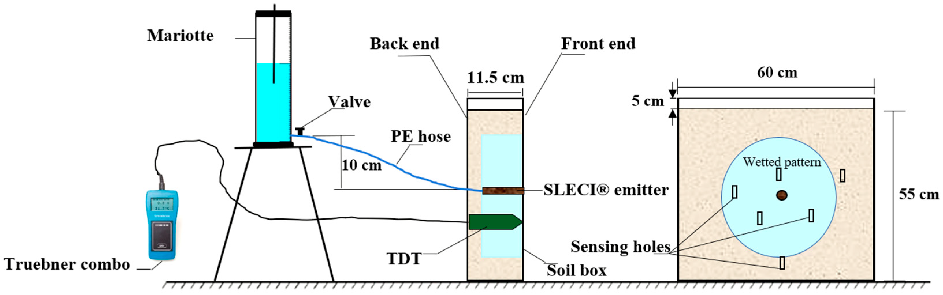
2.6. A Soil Box Laboratory Experiment

For the validation of the simulation, another laboratory experiment (hereafter referred to as a soil box experiment) was conducted to measure the key performance parameters of the SLECI system. The soil box measures 60.0 cm (width) × 11.5 cm (length) × 60.0 cm (height) and consisted of a transparent front panel made of polymethyl methacrylate (commonly known as Plexiglas) measuring 60.0 cm × 60.0 cm, allowing for the advancing wetting front to be observed during irrigation. The experiment layout consisted of the SLECI system, which included a vertical control assembly with a Mariotte bottle (Diameter = 7.1 cm; Volume = 1.0 L) serving as an overhead storage tank, and a SLECI emitter located at the transparent front panel end of the soil box.

The SLECI system is depicted in Figure 5. A SLECI emitter was buried at a depth ${\mathrm{D}}_{\mathrm{e}}$ of 30 cm and centred at the 30 cm width of the soil box. A TDT-based temperature and soil water sensor (Model: SMT-100, Truebner GmbH, Neustadt, Germany) was used to measure${ \theta }_v$ at various sensing holes on the soil box, and the average was computed. The locations of six (6) sensing holes are indicated in

Table 3. Locations of sensing holes in the soil box at which ${\theta }_v$ was measured during the experiment.

Point	x (cm)	y (cm)	Point	x (cm)	y (cm)
A	30	$-$50	D	34	$-$34
B	30	$-$20	E	30	$-$40
C	30	$-$25	F	22	$-$30

.

We performed a soil-specific calibration on the TDT sensor before it was used. Using an adjustable stand, the SLECI system was set up to supply irrigation water at a fixed h_op of 15 cm for ${\mathrm{t}}_{\mathrm{I}}$ = 48 h. To evaluate the performance of the SLECI system, parameters such as the wetting pattern (including the width of the vertical, ${\omega }_{\mathrm{z}}$, and horizontal fronts, ${\omega }_x$), volumetric water content ${ \theta }_v\left(H_p\right)$, and emitter discharge volume (${\mathrm{V}}_{\mathrm{e}}$), which represents the amount of water infiltrated into the soil, were measured during both the simulation and experiment. Assuming a symmetrical wetting front in both the $x$- and y-axis, the area of the wetted front, ${\mathrm{A}}_{\omega }$, was approximated to be ${\pi \omega }_{\mathrm{y}}{\omega }_x$, which holds for elliptic (${\omega }_x\ne$ ${\omega }_y$) and circular (${\omega }_x{=\omega }_y$) wetting fronts.

Preparation of the Soil Sample for the Soil Box Experiment

Debris were removed from the soil samples previously collected from a 100 cm depth, and larger particles were broken into smaller units, air-dried, and then sieved through a 3.25–mm sieve opening. The soil samples were then remoulded to dry bulk, ${\rho }_{\mathrm{d}-\mathrm{m}}$ of 1.34 $\mathrm{g}{ \mathrm{cm}}^{-3}$ and ${\theta }_{g-m}$ of 0.061${ \mathrm{g} \mathrm{g}}^{-1}$. The mass of the bulk soil sample, ${\mathrm{M}}_{\mathrm{m}}$ (which is about 53.96 kg), was weighed for remoulding and was determined using the following formula:

$${\mathrm{M}}_{\mathrm{m}}={\rho }_{\mathrm{d}-\mathrm{m}}(1+ {\theta }_{g-m}{)\mathrm{V}}_{\mathrm{b}}$$

(14)

where ${\mathrm{V}}_{\mathrm{b}}$ is the filled volume of the soil box, and ${\theta }_{g-m}$ is the average gravimetric water content of the soil (determined prior to remoulding). The soil was then remoulded in five successive 11 cm-thick layers. Each layer was manually compacted using a wooden plate (8.0 cm wide × 58.0 cm long × 4.3 cm thick, weighing 2.24 kg), which was raised to a height of 30 cm and allowed to fall freely under gravity onto the soil surface. This process was repeated until the soil box was filled to form a 55 cm soil column. The possibility of soil layer stratification was avoided by ensuring each compacted upper layer was adequately rough before the next soil layer was added and compacted.

Meanwhile, a SLECI emitter was installed at the 30 cm emitter burial depth and centred at the 30 cm width while soil sample was remoulded. Vaseline was smeared in layers on the interior wall of the transparent Plexiglas to prevent preferred flow along it. The soil’s initial volumetric water content was measured using the installed soil water sensor. Subsequently, the dynamic volumetric water content of the remoulded soil was measured during irrigation in the soil box using the soil moisture sensor.

2.7. Evaluating the Key Performance Parameters

2.7.1. Emitter Discharge in Soil, Soil Water Content, and Evaporation

The amount of water discharged by the SLECI emitter was measured noting the drop in the water column of the Mariotte bottle at the start and stop of irrigation. The volumetric water content ${\theta }_v (H_p$) was measured using the SMT-100 soil water sensor after water infiltration ceased. Meanwhile, the open water evaporation rates were measured by the weighing method.

2.7.2. Evaluating the Simulated Model

The performance of the model was tested by comparing the key performance parameters obtained by model simulation with the experimentally determined ones through the application of the normalised root mean square error (NRMSE), the mean relative error (MRE), Nash–Sutcliffe model efficiency coefficient (NSE), and the index of agreement (${\mathrm{I}}_{\mathrm{A}}$) introduced by [48].

$$\mathrm{NRMSE}={\displaystyle \frac{1}{{\mathrm{M}}_{\mathrm{avg}}}}\sqrt{{\displaystyle \frac{1}{\mathrm{N}}}{\sum }_{\mathrm{i}=1}^{\mathrm{N}}{\left({\mathrm{S}}_{\mathrm{i}}-{\mathrm{M}}_{\mathrm{i}}\right)}^2}$$

(15)

$$\mathrm{MRE}={\displaystyle \frac{1}{\mathrm{N}}}{\sum }_{\mathrm{i}=1}^{\mathrm{N}}{\displaystyle \frac{{(\mathrm{S}}_{\mathrm{I}}-{\mathrm{M}}_{\mathrm{i}})}{{\mathrm{M}}_{\mathrm{I}}}}$$

(16)

$$\mathrm{NSE}=1-{\displaystyle \frac{{\sum }_{\mathrm{i}=1}^{\mathrm{N}}{\left({\mathrm{S}}_{\mathrm{I}}-{\mathrm{M}}_{\mathrm{i}}\right)}^2}{{\sum }_{\mathrm{i}=1}^{\mathrm{N}}{\left({\mathrm{S}}_{\mathrm{I}}-{ \mathrm{M}}_{\mathrm{avg}}\right)}^2}}$$

(17)

$${\mathrm{I}}_{\mathrm{A}}=1-{\displaystyle \frac{{\sum }_{\mathrm{i}=1}^{\mathrm{N}}{\left({\mathrm{S}}_{\mathrm{I}}-{\mathrm{M}}_{\mathrm{i}}\right)}^2}{{\sum }_{\mathrm{i}}^{\mathrm{N}}{\left(\left|{\mathrm{S}}_{\mathrm{I} }-{ \mathrm{M}}_{\mathrm{avg}}\right|+\left|{\mathrm{M}}_{\mathrm{I}}-{\mathrm{M}}_{\mathrm{avg}}\right|\right)}^2}}$$

(18)

where $\mathrm{n}$ is the total number of data collected; ${\mathrm{S}}_{\mathrm{I}}$ and ${\mathrm{M}}_{\mathrm{I}}$ are the simulated and experimentally measured parametric values, respectively, at the $\mathrm{i}$th sample; ${\mathrm{M}}_{\mathrm{avg}}$ is the average of the experimentally measured parametric values; and $\mathrm{N}$ is the total number of measured points. The NRMSE points out the general measure of deviation degree between the experimentally measured parameters and the simulated ones. The MRE is a metric that specifies the bias with respect to overestimation or underestimation in the simulated parameters. The NSE provides an indication of model reliability. A prediction model is classified as “very good”, “good”, and “satisfactory” for a NSE > 0.80, 0.70 < NSE ≤ 0.80, and 0.50 < NSE ≤ 0.70, respectively [49]. The ${\mathrm{I}}_{\mathrm{A}}$ range is $0 \le {\mathrm{I}}_{\mathrm{A}} \le 1$, and the higher the ${\mathrm{I}}_{\mathrm{A}}$ value, the more strongly the simulated and experimentally measured values agree. A model is said to perform reasonably well if MRE$\approx$ 0, NRMSE $\approx$ 0 and ${\mathrm{I}}_{\mathrm{A}}$ $\cong$ 1.

2.7.3. Evaluating the SLECI System’s Key Performance Indices

The values from the prediction simulation were used to evaluate the performance of the SLECI system. The performance indices are the irrigation water application efficiency (${\epsilon }_{\mathrm{a}}$) [50], soil water distribution coefficient based on Christiansen’s uniformity (${\mathrm{CU}}_{\theta }$) [51], and the ratio of effective infiltrated volume (${\mathrm{r}}_{\mathrm{v}}$) [52]. These performance indices are expressed by Equations (19)–(21), as follows:

$${\epsilon }_{\mathrm{a}}=(1-{\displaystyle \frac{{\mathrm{D}}_{\mathrm{dp}}+{ \mathrm{D}}_{\mathrm{ev}}}{{\mathrm{D}}_{\mathrm{a}}}})\times 100$$

(19)

$${\mathrm{CU}}_{\theta }= \left(1-{\displaystyle \frac{1}{k}}{\displaystyle \frac{{\sum }_{k=1}^N\left|{\theta }_{v,k}-{\theta }_{v-\mathrm{avg}}\right|}{{\theta }_{v-\mathrm{avg}}}}\right)\times 100$$

(20)

$${\mathrm{r}}_{\mathrm{v}}={\displaystyle \frac{{\mathrm{A}}_{\mathrm{I}}}{{\mathrm{A}}_{\mathrm{T}}}}$$

(21)

where ${\mathrm{D}}_{\mathrm{a}}$ is the equivalent depth of irrigation water applied; ${\mathrm{D}}_{\mathrm{dp}}$ is the depth of irrigation water lost to deep percolation;${ \mathrm{D}}_{\mathrm{ev}}$ is the depth of irrigation water loss in surface evaporation, including the depth of basic surface evaporation; ${\theta }_{v,k}$ is the soil water content of wetted soil for the $k$^th measured sample; ${\theta }_{v-\mathrm{avg}}$ is the average soil volumetric water content at the root zone; $\mathrm{N}$ is the number of samples measured; ${\mathrm{A}}_{\mathrm{I}}$ is the area of water at the infiltrated region; and ${\mathrm{A}}_{\mathrm{T}}$ is the total root zone area. Using COMSOL’s logical expression, the ${\mathrm{r}}_{\mathrm{v}}$values were obtained by integrating the ratio of the 2D domain where ${\theta }_v$ ≥ ${\theta }_{v-\mathrm{FC}}$ to ${\mathrm{A}}_{\mathrm{T}}$ ($={½[\mathrm{E}}_{\mathrm{s}}{\mathrm{D}}_y-{\displaystyle \frac{\pi }{4}}{\mathrm{d}}_{\mathrm{o}}^2]$).

2.7.4. Interpretation of the Key Performance Indices

The performance criterion ${\mathrm{CU}}_{\theta }$ based on the guidelines provided by [53] for a drip irrigation system is represented in

Table 4. Performance evaluation criteria for the irrigation system based on the standard ${\mathrm{CU}}_{\theta }$ values.

${\mathbf{CU}}_{\mathit{\theta }}$ Range	Remark
<0.60	Unacceptable
0.60 ≤${ \mathrm{CU}}_{\theta }$ < 0.70	Weak
0.70 ≤ ${\mathrm{CU}}_{\theta }$ < 0.80	Moderate
0.80 ≤ ${\mathrm{CU}}_{\theta }$ < 0.90	Good
0.90 ≤ ${\mathrm{CU}}_{\theta }$ < 1.00	Excellent

Note(s): Adopted from [53].

. Generally, an ${\epsilon }_{\mathrm{a}}$ of 0.800 or higher is considered suitable [46]. Also, a higher ${\epsilon }_{\mathrm{a}}$ and ${\mathrm{r}}_{\mathrm{a}}$ are desirable as they indicate efficient water delivery to plant root zone. However, ${\mathrm{r}}_{\mathrm{v}}$ must be balanced against the need to minimise deep percolation and evaporation losses [54].

2.8. Multi-Objective Optimisation for the SLECI System

An epsilon-constraint multi-objective optimisation technique [55] was employed to determine the optimal h_op–D_e pair for operating the SLECI system in sandy loam. The goal is to maximise the key performance indices of the SLECI, specifically ${\mathrm{r}}_{\mathrm{v}}$, while ensuring the constrains ${\epsilon }_{\mathrm{a}} \ge 0.950$ and ${\mathrm{CU}}_{\theta } \ge 0.800$ are satisfied for a modelled soil profile depth (${\mathrm{Z}}_{\mathrm{r}}$) of 100 cm. The decision variables are the operating pressure head, ${\mathrm{h}}_{\mathrm{op}}$, and emitter burial depth, ${\mathrm{D}}_{\mathrm{e}}$. Accordingly, the following expression were used:

Objective function:

$$\mathrm{Maximise} f_1^{\prime }\left({\mathrm{h}}_{\mathrm{op}}, {\mathrm{D}}_{\mathrm{e}}\right)={\mathrm{r}}_{\mathrm{v}}\left({\mathrm{h}}_{\mathrm{op}}, {\mathrm{D}}_{\mathrm{e}}\right)$$

(22)

Constraints:

$$f_2^{\prime }\left({\mathrm{h}}_{\mathrm{op}}, {\mathrm{D}}_{\mathrm{e}}\right)={\epsilon }_{\mathrm{a}}\left({\mathrm{h}}_{\mathrm{op}}, {\mathrm{D}}_{\mathrm{e}}\right) \ge 0.950$$

(23)

$$f_3^{\prime }\left({\mathrm{h}}_{\mathrm{op}}, {\mathrm{D}}_{\mathrm{e}}\right)={\mathrm{CU}}_{\theta }\left({\mathrm{h}}_{\mathrm{op}}, {\mathrm{D}}_{\mathrm{e}}\right) \ge 0.800$$

(24)

Decision variable domains:

$${\mathrm{Z}}_{\mathrm{r}} \in \left\{100 \mathrm{cm}\right\}$$

(25)

$${\mathrm{h}}_{\mathrm{op}} \in \left\{25 \mathrm{cm}, 50 \mathrm{cm}, 75 \mathrm{cm}, 100 \mathrm{cm}, 125 \mathrm{cm}, 150 \mathrm{cm}\right\}$$

(26)

$${\mathrm{D}}_{\mathrm{e}} \in \left\{10 \mathrm{cm}, 20 \mathrm{cm}, 30 \mathrm{cm}, 40 \mathrm{cm}, 50 \mathrm{cm}, 60 \mathrm{cm}\right\}$$

(27)

Bounds:

$${0.800\le \mathrm{CU}}_{\theta }{(\mathrm{h}}_{\mathrm{op}}, {\mathrm{D}}_{\mathrm{e}})\le 1.000$$

(28)

$${0.950\le \epsilon }_{\mathrm{a}}{(\mathrm{h}}_{\mathrm{op}}, {\mathrm{D}}_{\mathrm{e}})\le 1.000$$

(29)

$${0.800 \le \mathrm{r}}_{\mathrm{v}} {(\mathrm{h}}_{\mathrm{op}}, {\mathrm{D}}_{\mathrm{e}}) \le 1.000$$

(30)

The optimal De–h_op pair is then determined by selecting the pair with the highest ${\mathrm{CU}}_{\theta }$ value, ranking it as the optimal performing combination.

2.9. Statistical Analyses

An analysis of variance (ANOVA) was carried out at α = 0.05 to verify the level of fit of the Richards equation 2D-model with respect to the entire dataset and to determine the how operating pressure head and emitter burial depth influence the responses. Where the difference in means was significant (p < 0.05), Tukey’s honest significance difference (HSD) test was performed. Python (version 3.9.13) and Microsoft Excel were used for processing the data and generating graphs.

3. Results and Discussions

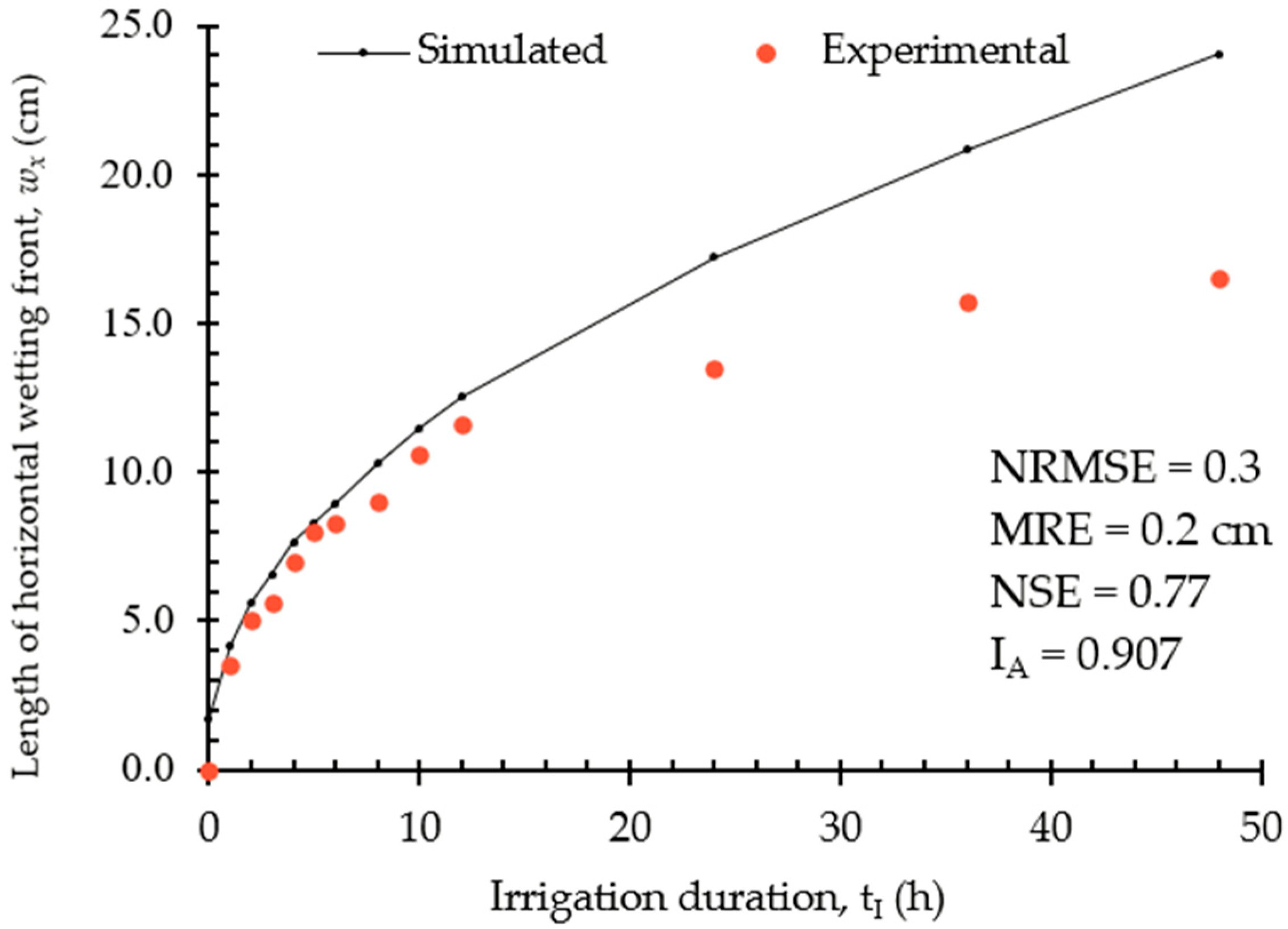
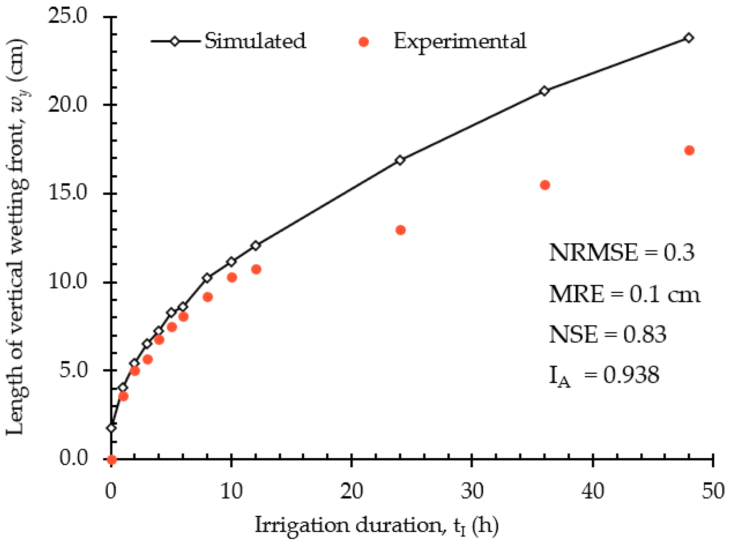
3.1. Validation of the COMSOL-2D Model

The comparison between experimentally measured and simulated values of soil water content, cumulative infiltrated volume, the lengths of the horizontal, and vertical wetting fronts are presented in Figure 6, Figure 7 and Figure 8, respectively.

A good agreement is observed between the experimental and simulated values of the soil average water content with performance indices of ${\mathrm{I}}_{\mathrm{A}}=$ 0.991, NRMSE = 0.013, MRE = 0.011 ${\mathrm{cm}}^3{ \mathrm{cm}}^{-3}$, and NSE = 0.97. For the cumulative infiltrated volume, the values of ${\mathrm{I}}_{\mathrm{A}}=$ 0.992, NRMSE = 0.2, MRE = $-$0.2 mL, and NSE = 0.97 were obtained, demonstrating good agreement between experimental and simulated measurements. Similarly, good agreements were observed between the simulated and measured lengths of the horizontal and vertical wetting fronts, with respective ${\mathrm{I}}_{\mathrm{A}}$, at 0.907 and 0.938, NRMSE at 0.3 and 0.3, MRE 0.2 cm and 0.1 cm, and NSE at 0.77 and 0.83. Generally, the shapes of the wetting fronts were close to that of an ellipse. These observations are consistent with research findings [56,57,58] specifically for sandy loam. At the onset of irrigation, both the vertical and horizontal wetting fronts advanced rapidly but slowed as soil water infiltration continued (Figure 8 and Figure 9). This behaviour can be explained by the initial high water potential gradient between the dry soil and the applied water, which tends to diminish as the soil moisture content increases. The model underestimated the cumulative infiltrated volume, but overestimated the soil water content (only slightly, with less than 1.0% deviation) and the lengths of the vertical and horizontal wetting fronts. The discrepancies between the measured and simulated values for both the length of vertical and wetting fronts can be explained by the fact that free drainage (mainly driven by gravity) becomes more profound compared to capillary rise, especially at extended irrigation durations [34].

However, the NSE values were all greater than 0.80 (except for that of the length of the horizontal wetting front, which was 0.77 and close to 0.80), and all ${\mathrm{I}}_{\mathrm{A}}$ values are approximately equal to 1.0 for all the four simulated and experimentally measured parameters; hence, the underestimation and overestimation can be considered as insignificant. These results indicate that the COMSOL-2D model simulation reliably predicted the soil water content, cumulative infiltrated volume, and the lengths of the horizontal and vertical wetting fronts when sandy loam is irrigated using the SLECI system. The initial deviation between measured and simulated cumulative discharge is explained by the usual unsteady potential difference between the interior and exterior walls at the start of irrigation [33]. The open water surface evaporation and soil temperature measured during the soil box experiment is presented in Figure 10. As expected, as the soil temperature increases, a greater depth of water is lost to evaporation and vice versa.

3.2. Predicted Variables Versus Different System Operating Parameters

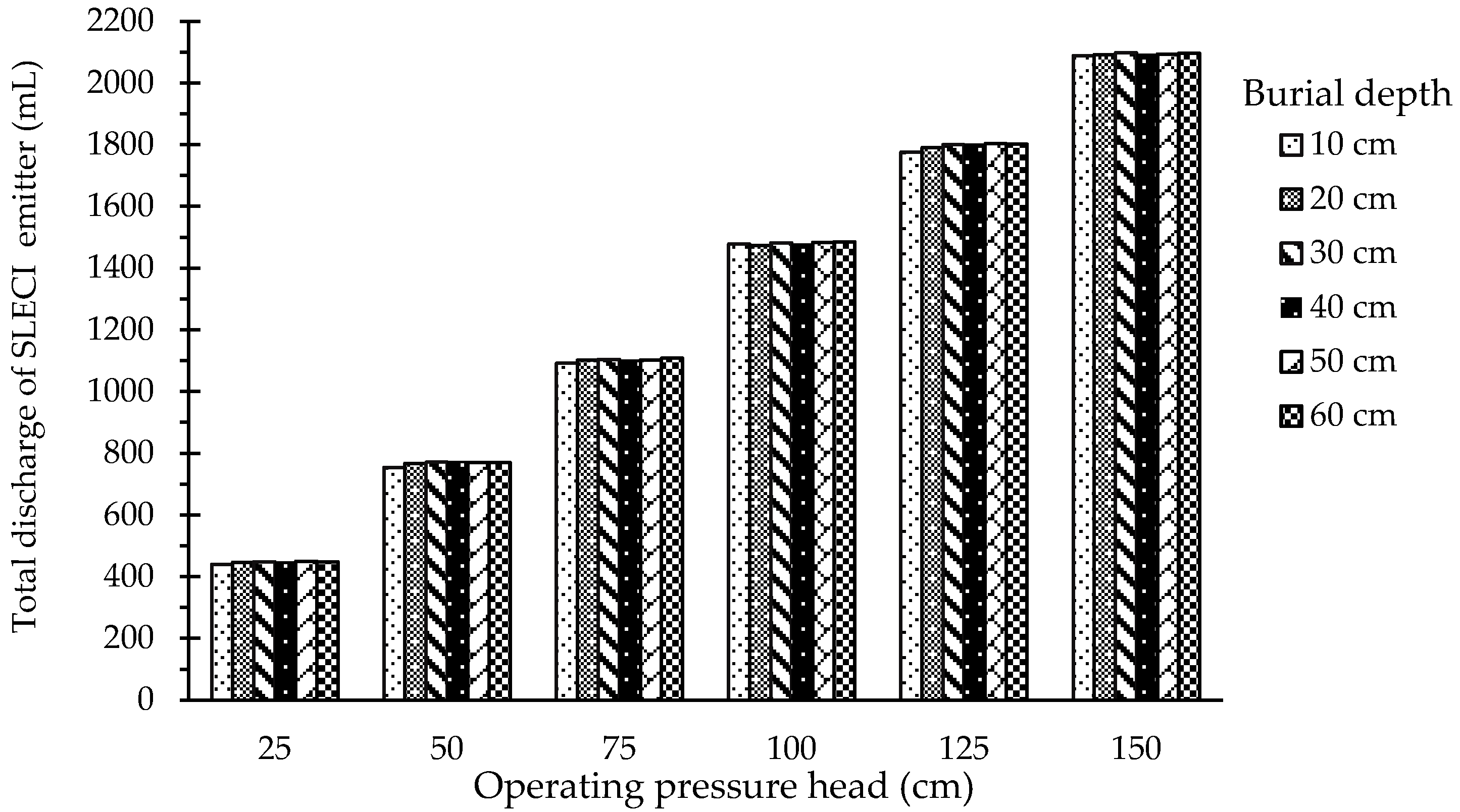
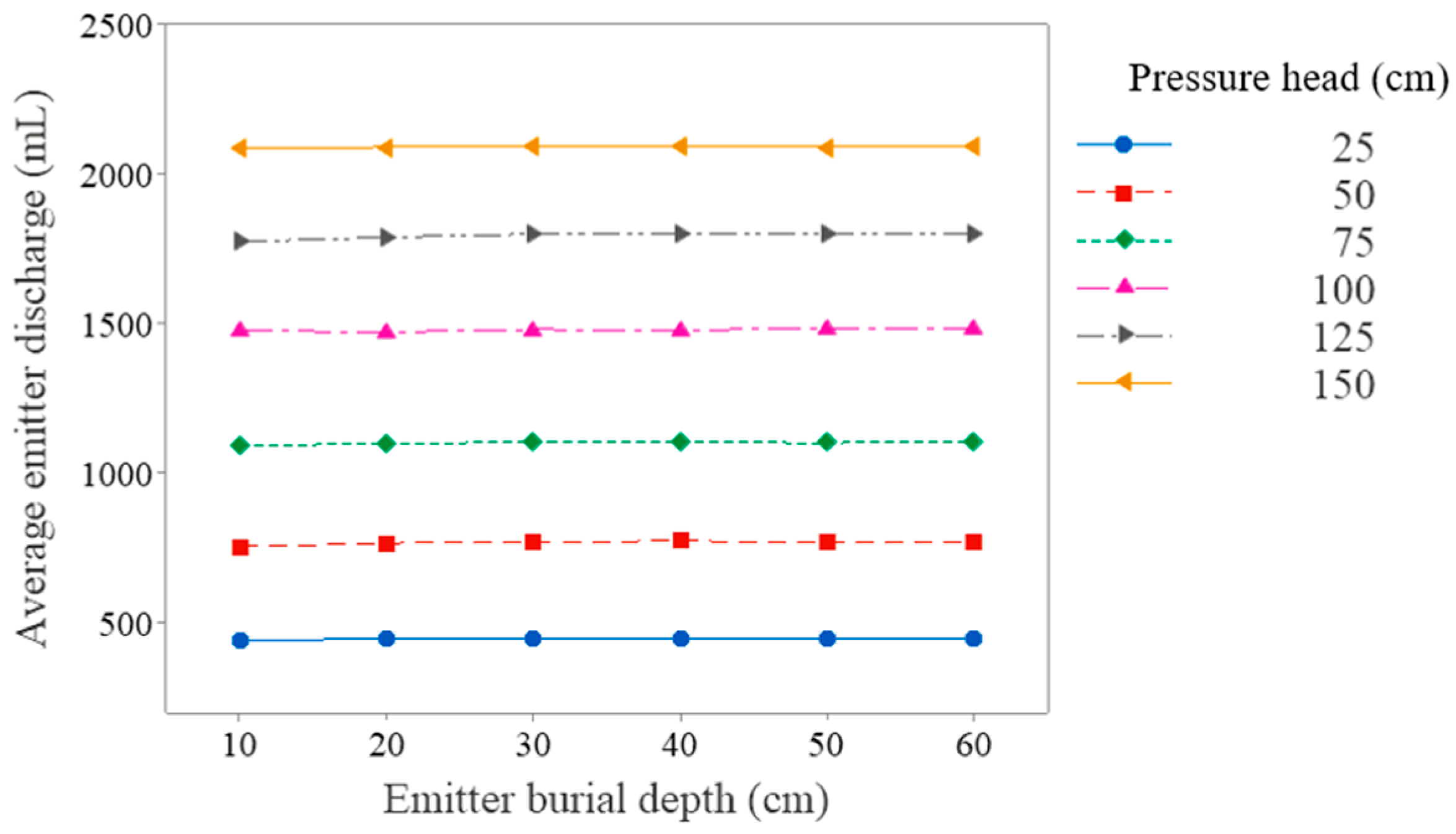
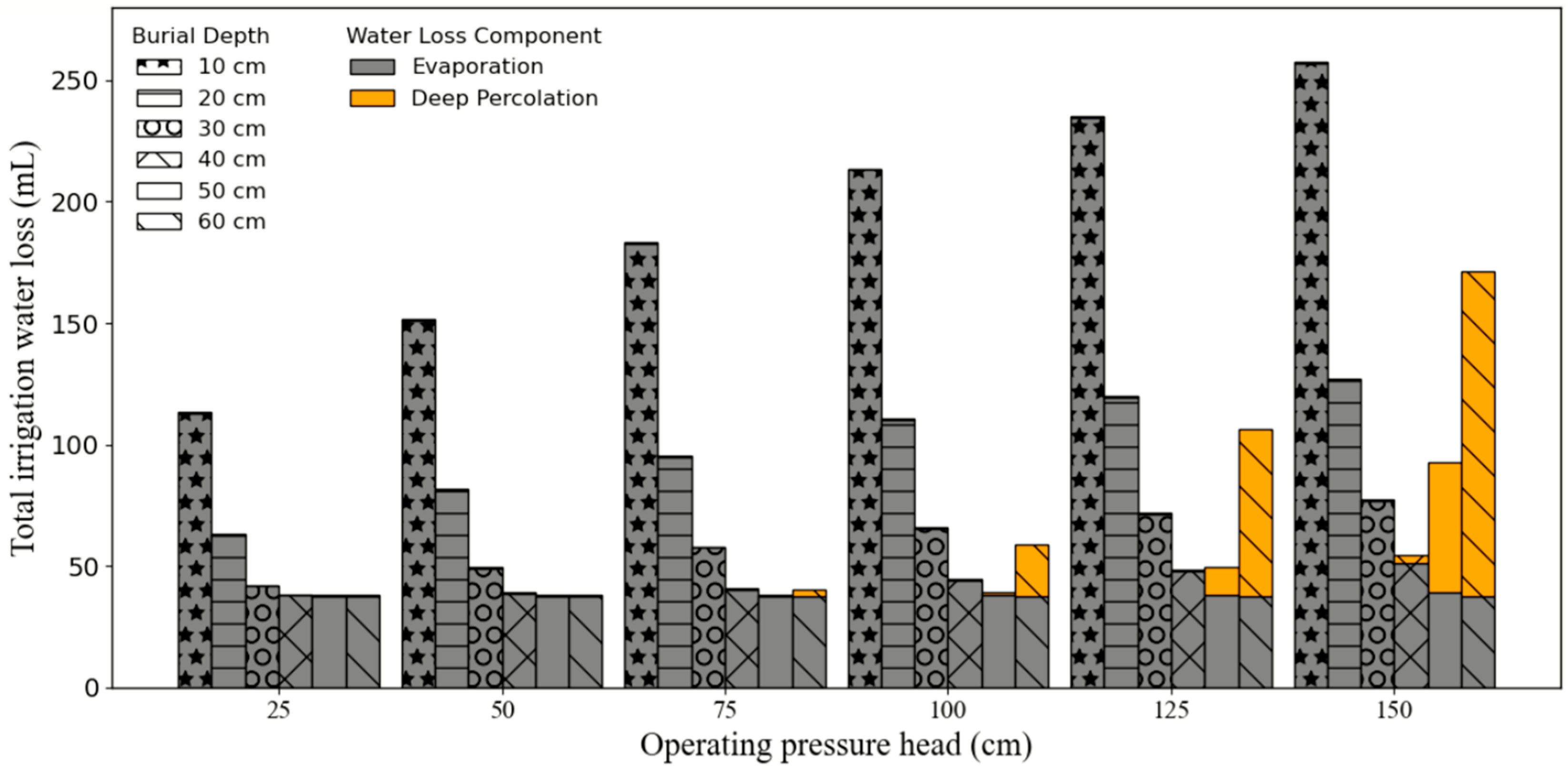
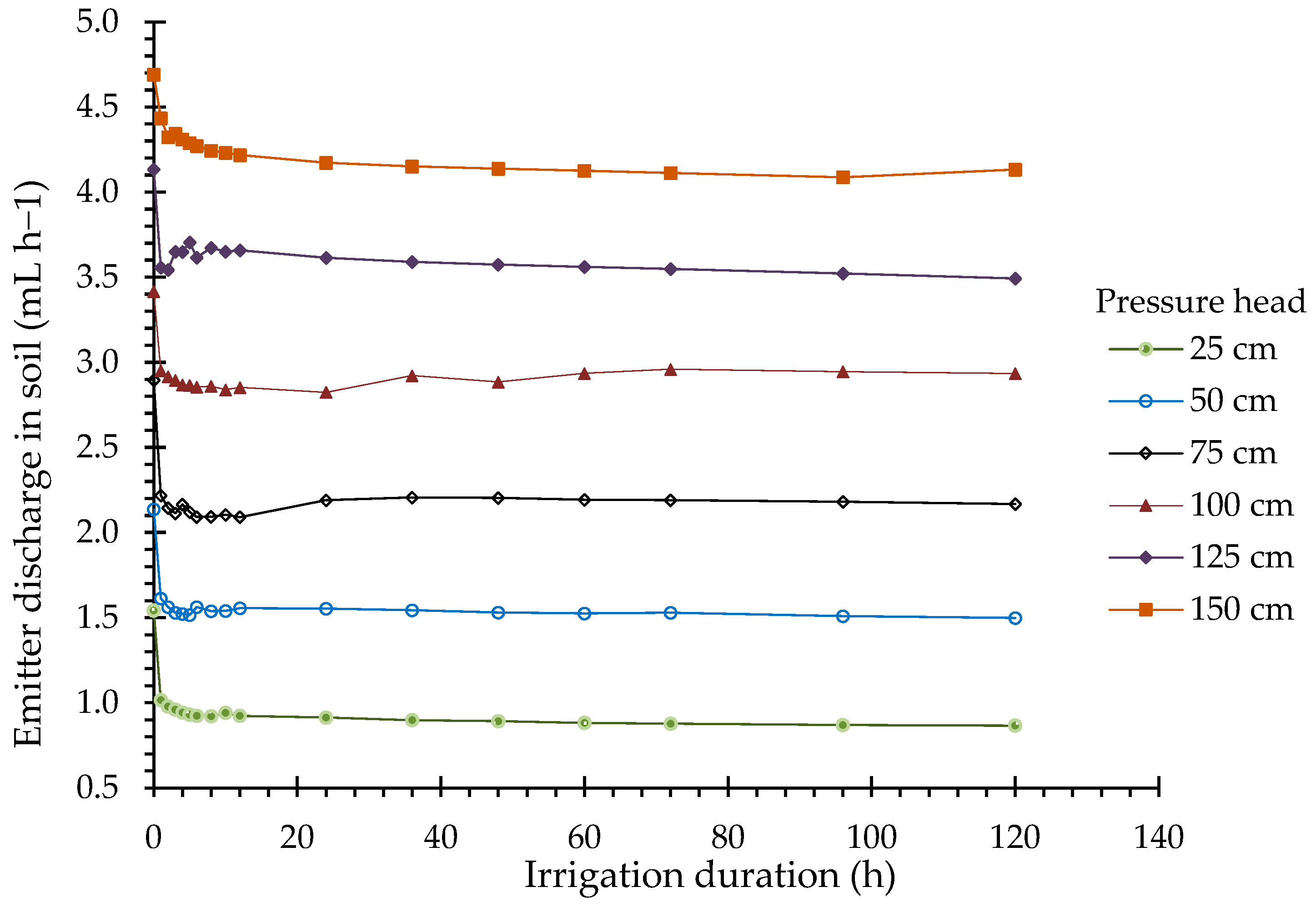
3.2.1. SLECI Emitter Operating Head and Burial Depth

Figure 11 provides insights into the relationship between the operating pressure head and the total discharge of the SLECI emitter measured across varying burial depths (10 cm to 60 cm) after irrigating for 120 h.

When the SLECI emitter is operated in a soil medium, the volume of irrigation water discharged will be the same as the volume of water infiltrated into the soil. The total discharge increased in the order of increasing operating pressure head (25 cm < 50 cm < 75 cm < 100 cm < 125 cm < 150 cm), and the differences were statistically significant (p < 0.5) across operating pressure heads. For a fixed operating pressure head, and across varying burial depths, the total discharge remains nearly the same, with no significant difference (p > 0.5). Also, there were no significant differences in emitter discharge among burial depth (p > 0.5) groups. This observation indicates that the buried depth of the SLECI emitter did not have a significant effect on the predicted total emitter discharge compared to the operating pressure head (see Figure 12).

The authors in Ref. [59] also reported similar findings based on Hydrus 2D simulation, noting that the operating pressure head was the most influential factor that determined emitter discharge and not the emitter burial depth. The interactions between burial depth and operating pressure head groups and their effects on emitter discharge is shown in Figure 12, further highlighting and confirming these trends. The independence of emitter discharge on burial depth suggests that the key parameter that regulates emitter discharge is the operating pressure head, while the emitter burial depth can be selected based on other factors like soil type or the plant’s root zone depth.

For each operating pressure head, the discharge tends to vary slightly across varying burial depths. At a lower pressure head (e.g., 25 cm and 50 cm), the variations in discharge across burial depths are minimal. However, at higher pressure heads (e.g., 125 cm and 150 cm), the difference between discharge values for varying burial depths become more pronounced. At deeper burial depths (e.g., from 50 cm to 60 cm), the discharge appears to reduce slightly compared to shallower burial depths (e.g., from 10 cm to 30 cm). This observation can be explained by the increase in soil water potential at deeper soil depths as a result of reduced soil permeability [60].

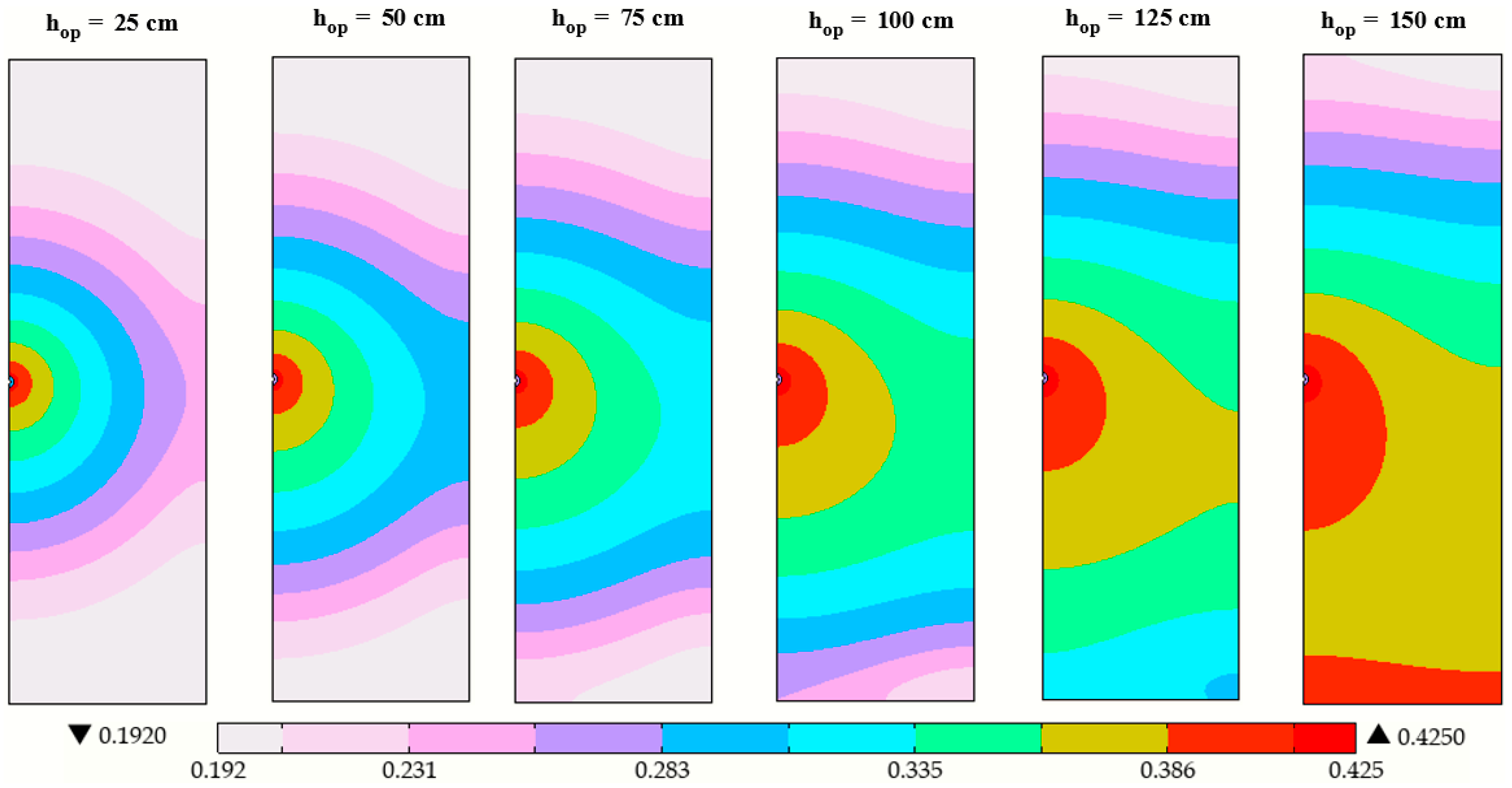
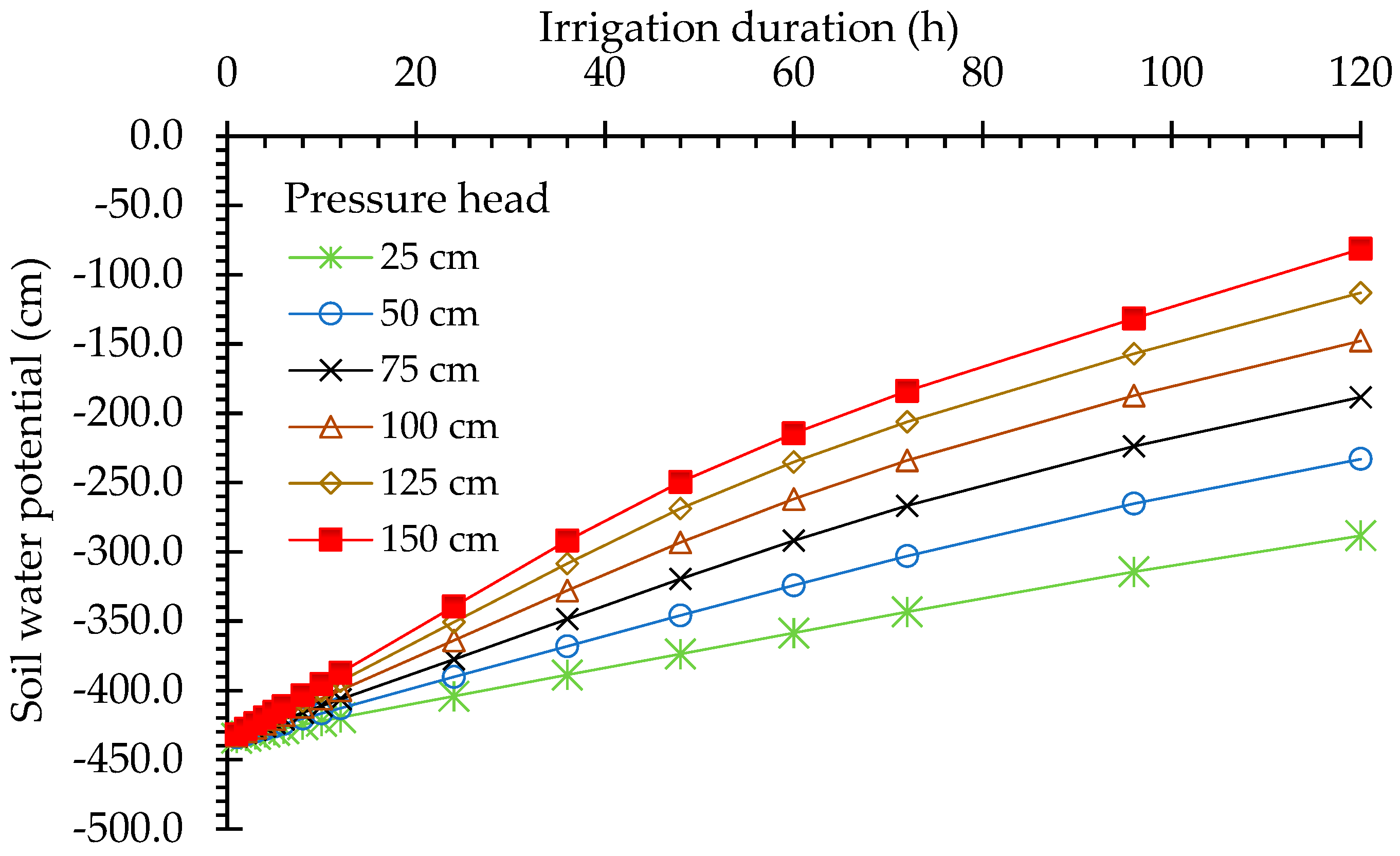
3.2.2. Effect of the Operating Pressure Head on the Advancement of the Water Front

The advancing wetting fronts within the modelled soil profile after 120 h of application of irrigation water across varying operating heads (25 cm to 150 cm) for an emitter burial depth of 50 cm are depicted in Figure 13.

The contour plots depict the distribution of volumetric water content. The colour scale shows water content ranging from 0.192 to 0.425. The red contours are indicative of saturated soil conditions near the emitter, with the yellow, green, and blue indicating progressively lower water content as the distance from the emitter increases. Higher operating pressure heads result in more pronounced advancement in wetting fronts (water distribution), spreading further in both horizontal and vertical directions within the soil profile. At lower operating pressure heads (e.g., 25 cm and 50 cm), the wetting front is more confined, showing a smaller horizontal and vertical spread. At higher operating pressure heads, the wetting front becomes more asymmetric, with a greater horizontal spread compared to the vertical fronts, similar to the results obtained in [58] for aeolian sandy soil and in [16], albeit using a vertical line source emitter. Deep percolation losses become more pronounced as the operating pressure head increases, reaching the highest at the 150 cm pressure head, as shown by the red contour at the bottom of the soil profile.

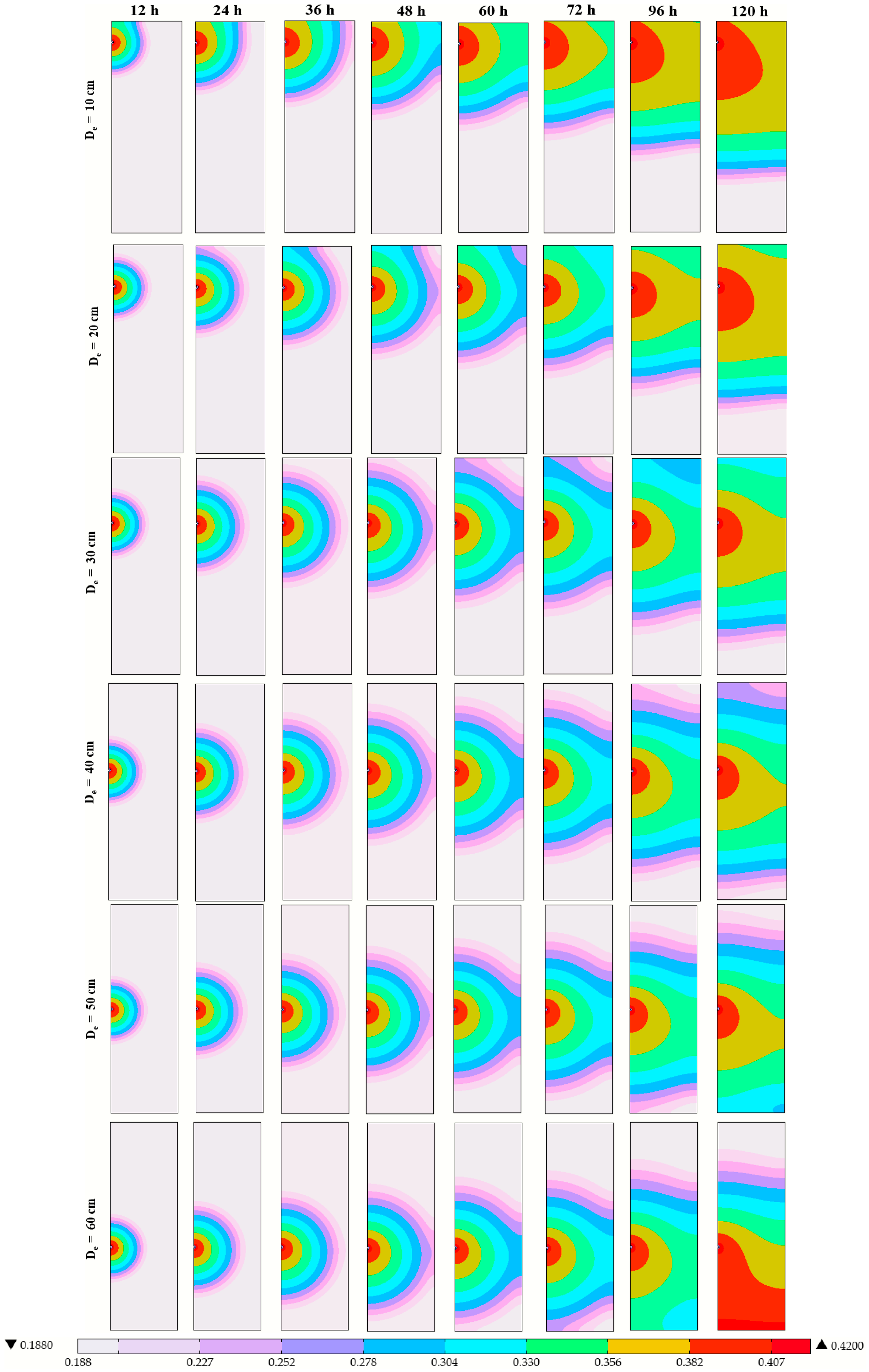
3.2.3. Simulated Wetted Front After 120 h for Emitter Burial Depths

The advancing wetting fronts at varying emitter burial depths, ${\mathrm{D}}_{\mathrm{e}}$ (10 cm to 60 cm), and irrigation durations (12 h to 120 h) for an initial water content of 0.189 are shown in Figure 14. Starting from 12 h, the wetting fronts exhibit similar geometric patterns across varying emitter burial depths and irrigation durations, and they appeared to be confined within the defined boundaries of the soil profile, except for the shallow emitter burial depths of 10 cm and 20 cm. The wetting front at these instances can be described as semi-circular in shape, indicating that the wetting fronts advanced at nearly the same velocities.

At shallow burial depths of 10 cm, 20 cm, and 30 cm, the upward vertical fronts reached the upper boundary after 12 h, 36 h, and 48 h, respectively. This indicates that evaporation losses become more significant at shallower emitter burial depths. Due to the influence of gravitational potential within the soil, the downward vertical fronts tend to advance faster compared to the upward fronts [61].

Also, it is observed that for an irrigation duration greater than or equal to 48 h, the wetting fronts all reached the right end of the soil profile’s boundary and tended to have an almost identical span across all emitter burial depths. At deeper emitter burial depths of 50 cm and 60 cm, the downward vertical wetting fronts reached the bottom boundary after 96 h and 72 h, respectively. Under these scenarios, deep percolation losses became significant, and the wetting fronts were characterised by distinct patterns and wider extents, which greatly impact IWUE during the field deployment of SSDI systems [62]. Based on the foregoing observations, it is evident that the SLECI emitter burial depth significantly influences the time taken for the wetting front to advance to the surface, right-end side, and bottom boundaries of the soil profile; hence, the installation of emitters at deeper depths must be avoided.

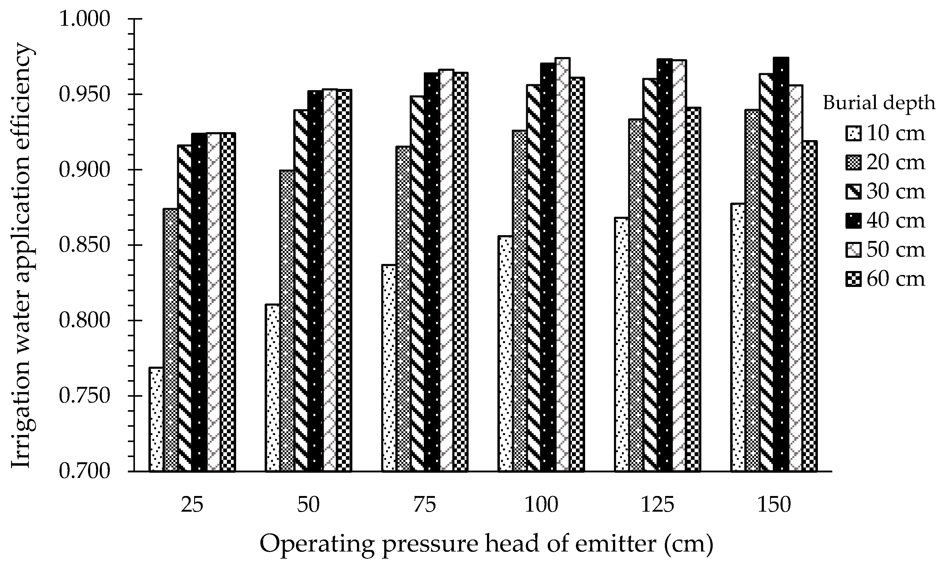
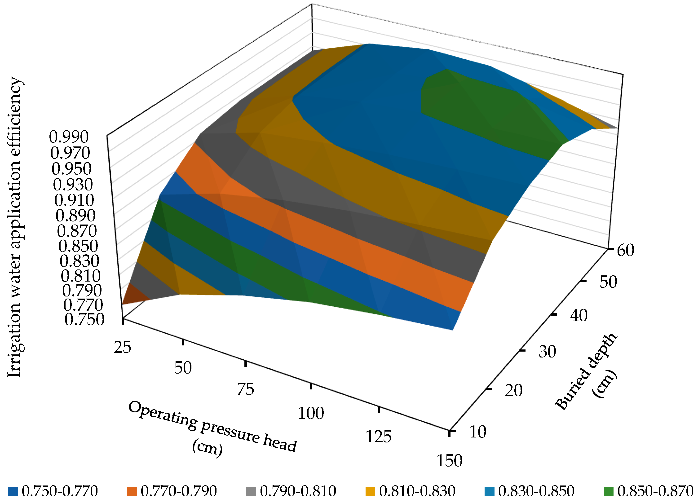
3.2.4. Key Performance Indices of the SLECI System

The irrigation water loss and irrigation water application efficiency are shown in Figure 15 for all treatment combinations. Lower irrigation water application efficiencies are observed at shallower emitter burial depths and vice versa. Evaporation water losses were larger at higher operating pressure heads, especially for shallower emitter burial depths, but decreases when emitters were buried deeper. As pointed out earlier, at deeper burial depths, the deep percolation water loss component becomes evident, especially at higher operating pressure heads. The lowest irrigation efficiency of 0.769 was observed for the shallowest burial depth of 10 cm and lowest operating pressure head of 25 cm. The highest irrigation efficiency of 0.974 was achieved at the maximum operating pressure head of 150 cm and a burial depth of 40 cm, where evaporation losses were minimal but deep percolation losses were relatively high (Figure 16). In general, irrigation water application efficiency decreases when both evaporation and percolation losses are significant. Similar trends and results were obtained by [28], with the lowest and highest water application efficiencies of approximately 0.750 and 1.000 at burial depths of 10 and 25 cm, respectively.

In contrast, in our study, the relatively low maximum water application efficiency is explained by the high hydraulic conductivity of the SLECI emitter and a deeper burial depth.

However, the largest discharges occur at the maximum operating pressure head of 150 cm (see Figure 11), resulting in the highest irrigation water application efficiencies, despite the relatively large deep percolation losses. The highest irrigation water application efficiencies were observed at emitter burial depths of 50 cm. Generally, irrigation efficiencies initially increase as emitter operating pressure heads increase, but these tend to decrease slightly at higher operating pressure heads.

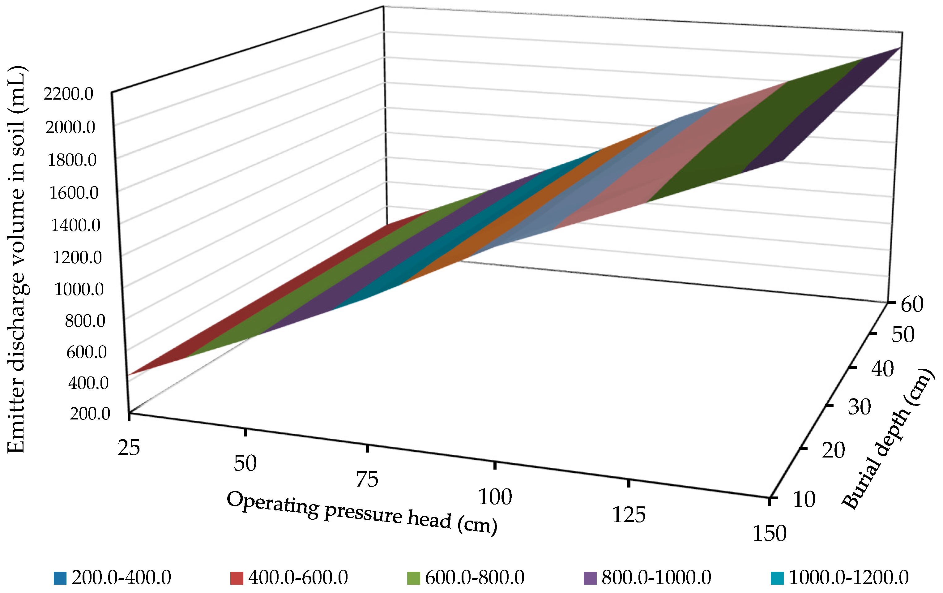
3.2.5. Soil Water Infiltration Under the Key Design Parameters of SLECI System

Figure 17 and Figure 18 show the changes in soil water potential and emitter discharge rate across varying emitter operating pressure heads, respectively.

To stay concise, only results for an emitter burial depth of 30 cm are presented; however, the same observations were made for the other emitter burial depths. It must be noted that, when the SLECI emitter is operated in a soil medium, the discharge rate will be the same as the soil’s infiltration rate. It can be observed that the discharge rate of the SLECI emitter is predominantly determined by the pressure head at which the emitter is operated. Over an increasing range of irrigation durations, the emitter discharge increases with operating pressure heads, peaking at the maximum pressure head of 150 cm. The increase in emitter discharge with increasing pressure head can be explained by the fact that the water potential difference between the interior and exterior walls ($∆\mathrm{h}$) of the SLECI emitter increases as operating pressure head rises. This trend in emitter discharge is similar across all remaining emitter burial depths for the same irrigation durations. When irrigation commenced, the discharges were relatively large but reduced sharply, and then they increased very slightly before finally reaching a steady rate. At the commencement of irrigation, the lowest values of soil water potential, equivalent to $-$431.7 cm, was observed when the soil was relatively dry. A low soil water content will lead to a high variation in $∆\mathrm{h}$, resulting in a large emitter discharge.

However, with the continuous application of irrigation water, the soil water content around the emitter increases, leading to a rise in soil water potential. As more portions of soil around the emitter become wetted, there is a significant reduction in $∆\mathrm{h}$. Consequently, the discharge from the emitter gradually decreases until a steady rate is reached when the immediate soil around the emitter nears saturation and the irrigation event approaches its end.

Generally, lower soil water potentials are observed at higher emitter operating pressure heads. A similar trend in soil water potential is observed when the SLECI emitter operates at the same pressure heads across the other burial depths. These observations are supported by similar findings in [63,64,65], although specific effects vary depending on soil texture and emitter placement.

3.3. Estimating the Optimal Performance Parameters of the SLECI System

3.3.1. A Predictive Model for the Water Infiltration Characteristics in Sandy Loam Under the SLECI System

To optimise the field installation parameters of the SLECI system, numerical models were developed for predicting the emitter discharge volume, ${\mathrm{V}}_{\mathrm{Qe}}$ (mL), and cumulative discharge, ${\mathrm{V}}_{\mathrm{T}-\mathrm{Qe}}$(mL), expressed by Equations (31) and (32), respectively, as follows:

$$\begin{gathered} {\mathrm{V}}_{\mathrm{Qe}}=0.219+ (5\times {10}^{-4}{\mathrm{D}}_{\mathrm{e}}+2.55\times {10}^{-2}{\mathrm{h}}_{\mathrm{op}}+{0.3113)\mathrm{t}}_{\mathrm{i}}+ \\ 4.6\times {10}^{-3}{\mathrm{h}}_{\mathrm{op}}; {\mathrm{R}}^2 = 1.000\hspace{1em}\hspace{1em}\hspace{1em}\hspace{1em}\hspace{1em}\hspace{1em} \end{gathered}$$

(31)

$$\begin{gathered} {\mathrm{V}}_{\mathrm{T}-\mathrm{Qe}}=163.5803+6\times {10}^{-4}{\mathrm{h}}_{\mathrm{op}}{\mathrm{D}}_{\mathrm{e}}+12.9764{\mathrm{h}}_{\mathrm{op}}+ \\ {0.1845\mathrm{D}}_{\mathrm{e}}; {\mathrm{R}}^2=0.999\hspace{1em}\hspace{1em}\hspace{1em}\hspace{1em}\hspace{1em} \end{gathered}$$

(32)

Equation (31) is valid for $0 {\le \mathrm{t}}_{\mathrm{i}} \le 120 \mathrm{h}$,$10 \mathrm{cm} \le {\mathrm{D}}_{\mathrm{e}} \le 60 \mathrm{cm}$, and $25 \mathrm{cm} \le {\mathrm{h}}_{\mathrm{op}} \le 150 \mathrm{cm}$, while Equation (32) is valid for the same range of values for ${\mathrm{D}}_{\mathrm{e}}$ and ${\mathrm{h}}_{\mathrm{op}}$ and ${ \mathrm{t}}_{\mathrm{i}} =120$ h. Figure 19 shows a 3D surface plot of the emitter cumulative discharge at varied operating pressure heads and emitter burial depths after 120 h, from which the predictive model in Equation (32) was obtained by curve fitting.

From Equation (32), it was observed that, the higher the operating pressure head (${\mathrm{h}}_{\mathrm{op}}$), burial depth (${\mathrm{D}}_{\mathrm{e}})$, and irrigation duration (${\mathrm{t}}_{\mathrm{I}}$), the greater the volume of water discharged by the emitter the in soil (${\mathrm{V}}_{\mathrm{T}-\mathrm{Qe}}$). Among the variable influencing emitter discharge, ${\mathrm{t}}_{\mathrm{I}}$ has the most significant impact since it the commonest term. In contrast, ${\mathrm{D}}_{\mathrm{e}}$ has a relatively minor effect on ${\mathrm{V}}_{\mathrm{Qe}}$, as indicated by its small coefficient. For example, for ${\mathrm{t}}_{\mathrm{I}}=$ 60 h and ${\mathrm{h}}_{\mathrm{op}}=$ 100 cm, the predicted ${\mathrm{V}}_{\mathrm{Qe}}$ was 172.6 mL for ${\mathrm{D}}_{\mathrm{e}}=$ 10 cm and 176.2 mL for ${\mathrm{D}}_{\mathrm{e}}=$ 60 cm. This represents only a 2% increase, demonstrating that ${\mathrm{D}}_{\mathrm{e}}$ has a much less influence on discharge compared to ${\mathrm{h}}_{\mathrm{op}}$, for which there is a 74% increase in discharge from 25 cm (minimum operating pressure head) to 150 cm (maximum operating pressure head) for ${\mathrm{D}}_{\mathrm{e}}=$ 60 cm for the same ${\mathrm{t}}_{\mathrm{i}}=$ 60 h.

Three (3) more predictive models were developed to predict the irrigation water application (${\epsilon }_{\mathrm{a}}$), soil water distribution efficiencies (${\mathrm{CU}}_{\theta })$, and ratio of effective infiltrated volume (${\mathrm{r}}_{\mathrm{v}}$) for sandy loam based on the 3D surface plots presented in Figure 20, Figure 21 and Figure 22, respectively.

The predictive equations for ${\epsilon }_{\mathrm{a}}$, ${\mathrm{CU}}_{\theta }$, and ${\mathrm{r}}_{\mathrm{v}}$ are expressed by Equations (33), (34), and (35), respectively, as follows:

$$\begin{gathered} {\epsilon }_{\mathrm{a}}=0.6433+1.9930 \times {{10}^{-3}\mathrm{h}}_{\mathrm{op}}+1.0761 \times {{10}^{-2}\mathrm{D}}_{\mathrm{e}}-6\times {10}^{-6}{\mathrm{h}}_{\mathrm{op}}^2-1.07\times {10}^{-4}{\mathrm{D}}_{\mathrm{e}}^2- \\ 1.5{ \times 10}^{-5}{\mathrm{h}}_{\mathrm{op}}{\mathrm{D}}_{\mathrm{e}}; {\mathrm{R}}^2=0.976\hspace{1em}\hspace{1em}\hspace{1em}\hspace{1em}\hspace{1em}\hspace{1em}\hspace{1em}\hspace{1em}\hspace{1em}\hspace{1em}\hspace{1em}\hspace{1em}\hspace{1em}\hspace{1em}\hspace{1em}\hspace{1em} \end{gathered}$$

(33)

$$\begin{gathered} {\mathrm{CU}}_{\theta } =0.9305 -8.3 \times {{10}^{-4}\mathrm{h}}_{\mathrm{op}}- 1.825 \times {{10}^{-3}\mathrm{D}}_{\mathrm{e}}-1 {\times 10}^{-6}{\mathrm{h}}_{\mathrm{op}}^2- \\ 2.2 {\times 10}^{-5}{\mathrm{D}}_{\mathrm{e}}^2; {\mathrm{R}}^2=0.980\hspace{1em}\hspace{1em}\hspace{1em}\hspace{1em}\hspace{1em}\hspace{1em}\hspace{1em}\hspace{1em}\hspace{1em} \end{gathered}$$

(34)

$${\mathrm{r}}_{\mathrm{v}}={0.08851\mathrm{h}}_{\mathrm{op}}^{0.39648}{\mathrm{D}}_{\mathrm{e}}^{0.09727}$$

(35)

These models are valid for $10 \mathrm{cm} \le {\mathrm{D}}_{\mathrm{e}} \le 60 \mathrm{cm}$ and 25$\mathrm{cm} \le {\mathrm{h}}_{\mathrm{op}} \le 150 \mathrm{cm}$ in sandy loam. The models expressed by Equations (31)–(35) can be used to predict ${{\mathrm{V}}_{\mathrm{Qe}}, \mathrm{V}}_{\mathrm{T}-\mathrm{Qe}}$, ${\epsilon }_{\mathrm{a}}$, ${\mathrm{CU}}_{\theta }$, ${\mathrm{r}}_{\mathrm{v}}$, and the performance of the SLECI system in sandy loam.

3.3.2. Multi-Objective Optimisation

The results from the multi-objective optimisation approach are presented in

Table 5. Ranking of the optimal operating pressure heads and burial depths for the SLECI system based on the total emitter discharge volume, soil water distribution coefficient, irrigation water application, and ratio of effective infiltrated volume for an effective rooting depth of 100 cm.

${\mathbf{h}}_{\mathbf{op}}$ (cm)	${\mathbf{D}}_{\mathbf{e}}$(cm)	${\mathbf{V}}_{\mathbf{T}-\mathbf{Qe}}$(mL)	${\mathbf{CU}}_{\mathit{\theta }}$	${\epsilon }_{\mathbf{a}}$	${\mathbf{r}}_{\mathbf{v}}$	${\mathbf{CU}}_{\mathit{\theta }}$ Class
125	40	422.6	0.807	0.973	0.948	Good
125	50	422.4	0.808	0.973	0.902	Good
100	40	353.9	0.825	0.970	0.865	Good
100	50	353.5	0.824	0.974	0.860	Good
125	30	420.6	0.809	0.960	0.849	Good

.

The optimal h_op–D_e pairs are ranked for the SLECI system based on ${\mathrm{CU}}_{\theta }$, ${\epsilon }_{\mathrm{a}}$, ${\mathrm{r}}_{\mathrm{v}}$, and their corresponding ${\mathrm{CU}}_{\theta }$ performance class. It can be seen from Table 4 that operating the SLECI system at h_op = 125 cm and D_e = 40 cm yielded ${\mathrm{V}}_{\mathrm{T}-\mathrm{Qe}}$ = 422.6 mL, ${\mathrm{CU}}_{\theta }$ = 0.807, ${\epsilon }_{\mathrm{a}}$ = 0.973, and ${\mathrm{r}}_{\mathrm{v}}$ = 0.948, which ranked the highest, accordingly, and provided the best balance between ${\epsilon }_{\mathrm{a}}$, ${\mathrm{CU}}_{\theta }$, and ${\mathrm{r}}_{\mathrm{v}}$.

4. Conclusions and Recommendations

This study has demonstrated that SLECI is a promising new method for subsurface irrigation. To optimise the performance of the SLECI system, we investigated the effects of the emitter burial depth and operating pressure head on the infiltration characteristics by evaluating the irrigation water application efficiency, water distribution uniformity, and ratio of effective infiltrated volume. Water flow under SLECI in sandy loam was successfully modelled using COMSOL Multiphysics, following the characterisation of the hydraulic parameters of the emitter. Validation against experimental data (soil water content, cumulative infiltrated volume, and the lengths of the horizontal and vertical wetting fronts) showed good agreement, supporting the reliability of the numerical model.

Further simulation at the initial soil water content corresponding to the management allowable revealed that the emitter operating pressure head significantly influenced infiltration characteristics, with higher pressure heads leading to greater emitter discharge rates and more extensive wetting front development due to larger differences in water potential between the interior and exterior of the emitter. In contrast, burial depth primarily determined the span of the vertical wetting fronts but had a negligible effect on emitter discharge and the velocity with which wetting fronts advanced. Based on these insights, a set of predictive numerical models were developed to estimate emitter discharge volume, irrigation distribution uniformity, and application efficiency (with emitter burial depths and operating pressure heads as variables) in sandy loam.

From the predictive models, we identified the optimal SLECI operating parameters for sandy loam as follows: an emitter pressure head of 125 cm and a burial depth of 40 cm are recommended for crops with an effective rootzone depth of 100 cm. If alternative design choices are needed, operating combinations that achieve a water distribution uniformity (${\mathrm{CU}}_{\theta })$ $\ge$ 0.800, an irrigation water application efficiency (${\epsilon }_{\mathrm{a}}$) $\ge$ 0.950, and a ratio of effective infiltrated volume (${\mathrm{r}}_{\mathrm{v}})\ge$0.800 should be selected.

These findings provide a strong basis for the design, practical field deployment, and operation of the SLECI system, offering a tool for enhancing water use efficiency in sandy loam soils. The numerical models developed here enable the rapid evaluation of SLECI performance under different design and management conditions, supporting more adaptive and sustainable irrigation practices.

Future research should expand this modelling approach to other soil textures and rooting depths, enabling the optimal design of the SLECI system for a wider range of crops and environmental conditions.

Ultimately, SLECI, supported by the optimisation framework established in this study, has the potential to contribute meaningfully to precision irrigation and water conservation efforts in agriculture.

References

1. Abbas, F.; Al-Naemi, S.; Farooque, A.A.; Phillips, M. A Review on the Water Dimensions, Security, and Governance for Two Distinct Regions. Water 2023, 15, 208. [Google Scholar] [CrossRef]
2. Mateo-Sagasta, J.; Zadeh, S.M.; Turral, H.; Burke, J. Water Pollution from Agriculture: A Global Review; The Food and Agricultural Organization: Rome, Italy, 2017; pp. 1–35. [Google Scholar]
3. Döll, P.; Schmied, H.M.; Schuh, C.; Portmann, F.T.; Eicker, A. Global-scale assessment of groundwater depletion and related groundwater abstractions: Combining hydrological modeling with information from well observations and GRACE satellites. Water Resour. Res. 2014, 50, 5698–5720. [Google Scholar] [CrossRef]
4. Siebert, S.; Burke, J.; Faures, J.M.; Frenken, K.; Hoogeveen, J.; Döll, P.; Portmann, F.T. Groundwater use for irrigation—A global inventory. Hydrol. Earth Syst. Sci. 2010, 14, 1863–1880. [Google Scholar] [CrossRef]
5. FAO. Food and Agriculture Organization Corporate Statistical Database. Available online: https://www.fao.org/aquastat/en/databases/maindatabase (accessed on 13 August 2023).
6. FAO. Water for Sustainable Food and Agriculture: A Report Produced for the G20 Presidency of Germany. Rome. Available online: https://www.fao.org/3/i7959e/i7959e.pdf (accessed on 20 March 2025).
7. Ghazouani, H.; Autovino, D.; Rallo, G.; Douh, B.; Provenzano, G. Using HYDRUS-2D model to assess the optimal drip lateral depth for Eggplant crop in a sandy loam soil of central Tunisia. Ital. J. Agrometeorol. 2016, 1, 47–58. [Google Scholar]
8. Zhang, H.; Wang, D.; Ayars, J.E.; Phene, C.J. Biophysical response of young pomegranate trees to surface and sub-surface drip irrigation and deficit irrigation. Irrig. Sci. 2017, 35, 425–435. [Google Scholar] [CrossRef]
9. Martínez-Gimeno, M.A.; Bonet, L.; Provenzano, G.; Badal, E.; Intrigliolo, D.S.; Ballester, C. Assessment of yield and water productivity of clementine trees under surface and subsurface drip irrigation. Agric. Water Manag. 2018, 206, 209–216. [Google Scholar] [CrossRef]
10. Consoli, S.; Stagno, F.; Roccuzzo, G.; Cirelli, G.L.; Intrigliolo, F. Sustainable management of limited water resources in a young orange orchard. Agric. Water Manag. 2014, 132, 60–68. [Google Scholar] [CrossRef]
11. Robles, J.M.; Botía, P.; Pérez-Pérez, J.G. Subsurface drip irrigation affects trunk diameter fluctuations in lemon trees, in comparison with surface drip irrigation. Agric. Water Manag. 2016, 165, 11–21. [Google Scholar] [CrossRef]
12. Dirwai, T.L.; Mabhaudhi, T.; Kanda, E.K.; Senzanje, A. Moistube irrigation technology development, adoption and future prospects: A systematic scoping review. Heliyon 2021, 7, e06213. [Google Scholar] [CrossRef]
13. Sechube, M.P.; Chaba, H.A.; Plooy, C.P.D.; Truter, M.; Araya, H. Evaluating the economic cost of the self-regulating, low energy, clay-based irrigation system as a climate-smart agricultural innovation for smallholder farmers, South Africa. In Evidence-Based Case Studies in South Africa; Department of Agriculture, Land Reform and Rural Development (DALRRD): Arcadia, South Africa, 2022; p. 209. [Google Scholar]
14. Kanda, E.K.; Senzanje, A.; Mabhaudhi, T. Soil water dynamics under Moistube irrigation. Phys. Chem. Earth 2020, 115, 102836. [Google Scholar] [CrossRef]
15. Pereira, D.; Leitao, J.C.C.; Gaspar, P.D.; Fael, C.; Falorca, I.; Khairy, W.; Wahid, N.; El Yousfi, H.; Bouazzama, B.; Siering, J.; et al. Exploring Irrigation and Water Supply Technologies for Smallholder Farmers in the Mediterranean Region. Sustainability 2023, 15, 6875. [Google Scholar] [CrossRef]
16. Fan, Y.; Ma, L.; Wei, H.; Zhu, P. Numerical investigation of wetting front migration and soil water distribution under vertical line source irrigation with different influencing factors. Water Sci. Technol. Water Supply 2021, 21, 2233–2248. [Google Scholar] [CrossRef]
17. Qiao, W.; Luo, Z.; Lin, D.; Zhang, Z.; Wang, S. An Empirical Model for Aeolian Sandy Soil Wetting Front Estimation with Subsurface Drip Irrigation. Water 2023, 15, 1336. [Google Scholar] [CrossRef]
18. Cristóbal-Muñoz, I.; Prado-Hernández, J.V.; Martínez-Ruiz, A.; Pascual-Ramírez, F.; Cristóbal-Acevedo, D.; Cristóbal-Muñoz, D. An Improved Empirical Model for Estimating the Geometry of the Soil Wetting Front with Surface Drip Irrigation. Water 2022, 14, 1827. [Google Scholar] [CrossRef]
19. Qin, X.; Duan, X.; Su, L.; Shen, X.; Hu, G. Numerical Simulation of Soil Water Movement under Subsurface Irrigation. Math. Probl. Eng. 2014, 2014, 126398. [Google Scholar] [CrossRef]
20. Al-Ogaidi, A.A.M.; Wayayok, A.; Rowshon, M.K.; Abdullah, A.F. Wetting patterns estimation under drip irrigation systems using an enhanced empirical model. Agric. Water Manag. 2016, 176, 203–213. [Google Scholar] [CrossRef]
21. Douh, B.; Didouni, O.; Mguidiche, A.; Ghazouani, H.; Khila, S.; Belaid, A.; Boujelben, A. Wetting patterns estimation under subsurface drip irrigation systems for different discharge rates and soil types. In Advances in Science, Technology and Innovation; Springer: Berlin/Heidelberg, Germany, 2018; pp. 877–878. [Google Scholar] [CrossRef]
22. Shiri, J.; Karimi, B.; Karimi, N.; Kazemi, M.H.; Karimi, S. Simulating wetting front dimensions of drip irrigation systems: Multi criteria assessment of soft computing models. J. Hydrol. 2020, 585, 124792. [Google Scholar] [CrossRef]
23. Fan, Y.; Yang, Z.; Wei, H. Establishment and verification of the prediction model of soil wetting pattern size in vertical moistube irrigation. Water Sci. Technol. Water Supply 2021, 21, 331–343. [Google Scholar] [CrossRef]
24. Karimi, R.; Appels, W.M. Soil moisture dynamics in a new indoor facility for subsurface drip irrigation of field crops. Irrig. Sci. 2021, 39, 715–724. [Google Scholar] [CrossRef]
25. Fan, Y.W.; Huang, N.; Zhang, J.; Zhao, T. Simulation of soil wetting pattern of vertical moistube-irrigation. Water 2018, 10, 601. [Google Scholar] [CrossRef]
26. Liu, X.; He, X.; Zhang, L. Simplified method for estimating discharge of microporous ceramic emitters for drip irrigation. Biosyst. Eng. 2022, 219, 38–55. [Google Scholar] [CrossRef]
27. Abid, H.N.; Abid, M.B. Predicting Wetting Patterns in Soil from a Single Subsurface Drip Irrigation System. J. Eng. 2019, 25, 41–53. [Google Scholar] [CrossRef]
28. Qi, W.; Zhang, Z.; Wang, C.; Huang, M. Prediction of infiltration behaviors and evaluation of irrigation efficiency in clay loam soil under Moistube® irrigation. Agric. Water Manag. 2021, 248, 106756. [Google Scholar] [CrossRef]
29. Lamm, F.R.; Ayars, J.E.; Nakayama, F.S. Microirrigation for Crop Production: Design, Operation, and Management; Elsevier: Amsterdam, The Netherlands, 2006. [Google Scholar]
30. Wang, J.; Huang, Y.; Long, H.; Hou, S.; Xing, A.; Sun, Z. Simulations of water movement and solute transport through different soil texture configurations under negative-pressure irrigation. Hydrol. Process 2017, 31, 2599–2612. [Google Scholar] [CrossRef]
31. Cai, Y.; Zhao, X.; Wu, P.; Zhang, L.; Zhu, D.; Chen, J. Effect of soil texture on water movement of porous ceramic emitters: A simulation study. Water 2018, 11, 22. [Google Scholar] [CrossRef]
32. Siyal, A.A.; Skaggs, T.H. Measured and simulated soil wetting patterns under porous clay pipe sub-surface irrigation. Agric. Water Manag. 2009, 96, 893–904. [Google Scholar] [CrossRef]
33. Cai, Y.; Wu, P.; Zhang, L.; Zhu, D.; Wu, S.; Zhao, X.; Chen, J.; Dong, Z. Prediction of flow characteristics and risk assessment of deep percolation by ceramic emitters in loam. J. Hydrol. 2018, 566, 901–909. [Google Scholar] [CrossRef]
34. Cai, Y.; Wu, P.; Zhang, L.; Zhu, D.; Chen, J.; Wu, S.; Zhao, X. Simulation of soil water movement under subsurface irrigation with porous ceramic emitter. Agric. Water Manag. 2017, 192, 244–256. [Google Scholar] [CrossRef]
35. Kandelous, M.M.; Šimůnek, J. Numerical simulations of water movement in a subsurface drip irrigation system under field and laboratory conditions using HYDRUS-2D. Agric. Water Manag. 2010, 97, 1070–1076. [Google Scholar] [CrossRef]
36. Malchev, S.; Kornov, G.; Hansmann, H. Innovative clay-based micro-irrigation system ‘SLECI’ (Self-regulating; Energy, L., Clay-based Irrigation): Preliminary results from cherry orchard trials. J. Agric. Food Environ. Sci. 2022, 76, 45–55. [Google Scholar] [CrossRef]
37. DIVAGRI. Available online: https://divagri.org/sleci/ (accessed on 5 May 2021).
38. Bear, J. Dynamics of Fluids in Porous Media; Courier Corporation: North Chelmsford, MA, USA, 1972. [Google Scholar]
39. Schaap, M.G.; Leij, F.J.; Van Genuchten, M.T. Rosetta: A computer program for estimating soil hydraulic parameters with hierarchical pedotransfer functions. J. Hydrol. 2001, 251, 163–176. [Google Scholar] [CrossRef]
40. FAO. Standard Operating Procedure for Soil Bulk Density, Cylinder Method; FAO: Rome, Italy, 2023. [Google Scholar] [CrossRef]
41. Farooq, Q.U.; Naqash, M.T.; Ahmed, A.T.; Khawaja, B.A. Optimization of Subsurface Smart Irrigation System for Sandy Soils of Arid Climate. Model. Simul. Eng. 2021, 2021, 9012496. [Google Scholar] [CrossRef]
42. COMSOL. The Subsurface Flow Module User’s Guide. 2023. Available online: https://doc.comsol.com/6.2/doc/com.comsol.help.ssf/SubsurfaceFlowModuleUsersGuide.pdf (accessed on 20 March 2025).
43. Van Genuchten, M.T. A closed-form equation for predicting the hydraulic conductivity of unsaturated soils. Soil Sci. Soc. Am. J. 1980, 44, 892–898. [Google Scholar] [CrossRef]
44. Mualem, Y. A new model for predicting the hydraulic conductivity of unsaturated porous media. Water Resour. Res. 1976, 12, 513–522. [Google Scholar] [CrossRef]
45. Liu, X.; Zhang, L.; Liu, Q.; Yang, F.; Han, M.; Yao, S. Subsurface irrigation with ceramic emitters: Optimal working water head improves yield, fruit quality and water productivity of greenhouse tomato. Sci. Hortic. 2023, 310, 111712. [Google Scholar] [CrossRef]
46. Doorenbos, J.; Pruitt, W.O. Crop Water Requirements; FAO Irrigation and Drainage Paper 24; FAO: Rome, Italy, 1984. [Google Scholar]
47. Naglič, B.; Kechavarzi, C.; Coulon, F.; Pintar, M. Numerical investigation of the influence of texture, surface drip emitter discharge rate and initial soil moisture condition on wetting pattern size. Irrig. Sci. 2014, 32, 421–436. [Google Scholar] [CrossRef]
48. Willmott, C.J. Some comments on the evaluation of model performance. Bull. Am. Meteorol. Soc. 1982, 63, 1309–1313. [Google Scholar] [CrossRef]
49. Moriasi, D.N.; Gitau, M.W.; Pai, N.; Daggupati, P. Hydrologic and water quality models: Performance measures and evaluation criteria. Trans. ASABE 2015, 58, 1763–1785. [Google Scholar]
50. Wang, Z.; Zerihun, D.; Feyen, J. General irrigation efficiency for field water management. Agric. Water Manag. 1996, 30, 123–132. [Google Scholar] [CrossRef]
51. Christiansen, J.E. The uniformity of application of water by sprinkler systems. Agric. Eng. 1941, 22, 89–92. [Google Scholar]
52. Qi, W.; Zhang, Z.Y.; Wang, C.; Chen, Y.; Zhang, Z.M. Crack closure and flow regimes in cracked clay loam subjected to different irrigation methods. Geoderma 2020, 358, 113978. [Google Scholar] [CrossRef]
53. ASAE. Field Evaluation of Micro-Irrigation Systems, 43rd ed.; ASAE: St. Joseph, MO, USA, 1996; pp. 756–761. [Google Scholar]
54. Eisenhauer, D.E.; Martin, D.L.; Heeren, D.M.; Hoffman, G.J. Irrigation Systems Management; American Society of Agricultural and Biological Engineers (ASABE): St Joseph, MO, USA, 2021. [Google Scholar]
55. Deb, K.; Sindhya, K.; Hakanen, J. Multi-objective optimization. In Decision Sciences; CRC Press: Boca Raton, FL, USA, 2016; pp. 161–200. [Google Scholar]
56. Li, Y.; Nie, W.-B.; Feng, Z.-J. Development of a soil wetting pattern estimation model for drip irrigation. Water Supply 2023, 23, 144–161. [Google Scholar] [CrossRef]
57. Vishwakarma, D.K.; Kumar, R.; Tomar, A.S.; Kuriqi, A. Eco-hydrological modeling of soil wetting pattern dimensions under drip irrigation systems. Heliyon 2023, 9, e18078. [Google Scholar] [CrossRef] [PubMed]
58. Alrubaye, Y.L.; Yusuf, B.; Mohammad, T.A.; Nahazanan, H.; Zawawi, M.A.M. Experimental and Numerical Prediction of Wetting Fronts Size Created by Sub-Surface Bubble Irrigation System. Sustainability 2022, 14, 11492. [Google Scholar] [CrossRef]
59. Wang, C.; Ye, J.; Zhai, Y.; Kurexi, W.; Xing, D.; Feng, G.; Zhang, Q.; Zhang, Z. Dynamics of Moistube discharge, soil-water redistribution and wetting morphology in response to regulated working pressure heads. Agric. Water Manag. 2023, 282, 108285. [Google Scholar] [CrossRef]
60. Kirkham, M.B. Principles of Soil and Plant Water Relations; Elsevier: Amsterdam, The Netherlands, 2023. [Google Scholar]
61. Sun, Q.; Wang, Y.; Chen, G.; Yang, H.; Du, T. Water use efficiency was improved at leaf and yield levels of tomato plants by continuous irrigation using semipermeable membrane. Agric. Water Manag. 2018, 203, 430–437. [Google Scholar] [CrossRef]
62. Mattar, M.A.; El-Abedin, T.K.Z.; Al-Ghobari, H.M.; Alazba, A.A.; Elansary, H.O. Effects of different surface and subsurface drip irrigation levels on growth traits, tuber yield, and irrigation water use efficiency of potato crop. Irrig. Sci. 2021, 39, 517–533. [Google Scholar] [CrossRef]
63. Jia, M.; Wei, S.; Zhang, F.L.Y.; Shen, Y. Influence of soil texture and drip emitter flow rate on soil water movement under subsurface drip irrigation. Chin. J. Eco-Agric. 2025, 33, 749–758. [Google Scholar]
64. Zamani, S.; Fatahi, R.; Provenzano, G. A comprehensive model for hydraulic analysis and wetting patterns simulation under subsurface drip laterals. Water 2022, 14, 1965. [Google Scholar] [CrossRef]
65. Kandelous, M.M.; Šimůnek, J.; Van Genuchten, M.T.; Malek, K. Soil water content distributions between two emitters of a subsurface drip irrigation system. Soil Sci. Soc. Am. J. 2011, 75, 488–497. [Google Scholar] [CrossRef]
Figure 1. Picture of the clay-based SLECI emitter. (a) SLECI emitters with a 6 mm polyethylene (PE) hose connection and barb; and (b) hollow SLECI emitters with no hose connected. Source: [37].
Water 17 02058 g001
Figure 2. Model of water flow through the SLECI emitter buried in a soil medium. Source: adapted from [37].
Water 17 02058 g002
Figure 3. SLECI emitter discharges at various working pressure heads in an air medium.
Water 17 02058 g003
Figure 4. Mesh configuration and fitted boundary conditions deployed in Richards’ equation model builder simulation.
Water 17 02058 g004
Figure 5. Setup of the soil box experiment.
Water 17 02058 g005
Figure 6. Simulated and measured soil water content.
Water 17 02058 g006
Figure 7. Simulated and measured cumulative infiltration volume.
Water 17 02058 g007
Figure 8. Simulated and experimental measured length of the horizontal wetting fronts.
Water 17 02058 g008
Figure 9. Simulated and experimental measured length of the vertical wetting fronts.
Water 17 02058 g009
Figure 10. Measured evaporation depth and soil temperature during the soil box experiment.
Water 17 02058 g010
Figure 11. Total discharge of the SLECI emitter after irrigating for 120 h for varying emitter buried depths and operating pressure heads.
Water 17 02058 g011
Figure 12. Interaction plot showing the effect of the emitter operating pressure head and burial depth on the emitter discharge.
Water 17 02058 g012
Figure 13. Advancing wetting fronts within the modelled soil profile after 120 h of irrigation at an initial water content of 0.189. For conciseness, only treatments with an emitter buried at 50 cm are presented.
Water 17 02058 g013
Figure 14. Advancing wetting fronts within the modelled soil profile at varying irrigation durations and emitter burial depths. For conciseness, only treatments with an operating pressure head of 125 cm are presented.
Water 17 02058 g014
Figure 15. Irrigation water application efficiency under varied emitter buried depths and operating pressure heads for all treatments.
Water 17 02058 g015
Figure 16. Irrigation water application loss component under varied emitter buried depths and operating pressure heads for all treatments.
Water 17 02058 g016
Figure 17. Emitter discharge at varied operating pressure heads and a burial depth of 30 cm.
Water 17 02058 g017
Figure 18. Soil water potential at varied operating pressure heads and a burial depth of 30 cm. The emitter buried depth served as the reference point for soil water potential energy.
Water 17 02058 g018
Figure 19. Steady emitter discharge volume at varied operating pressure heads and emitter burial depths after 120 h.
Water 17 02058 g019
Figure 20. Average irrigation water application efficiency for all treatment combinations.
Water 17 02058 g020
Figure 21. Soil water distribution uniformity for all treatment combinations.
Water 17 02058 g021
Figure 22. Ratio of effective infiltrated volume for all treatments after 120 h.
Water 17 02058 g022