An Accuracy Assessment of the ESTARFM Data-Fusion Model in Monitoring Lake Dynamics

Abstract

High-spatiotemporal-resolution remote sensing data are of great significance for surface monitoring. However, existing remote sensing data cannot simultaneously meet the demands for high temporal and spatial resolution. Spatiotemporal fusion algorithms are effective solutions to this problem. Among these, the ESTARFM (Enhanced Spatiotemporal Adaptive Reflection Fusion Model) algorithm has been widely used for the fusion of multi-source remote sensing data to generate high spatiotemporal resolution remote sensing data, owing to its robustness. However, most existing studies have been limited to applying ESTARFM for the fusion of single-surface-element data and have paid less attention to the effects of multi-band remote sensing data fusion and its accuracy analysis. For this reason, this study selects Chagan Lake as the study area and conducts a detailed evaluation of the performance of the ESTARFM in fusing six bands—visible, near-infrared, infrared, and far-infrared—using metrics such as the correlation coefficient and Root Mean Square Error (RMSE). The results show that (1) the ESTARFM fusion image is highly consistent with the clear-sky Landsat image, with the coefficients of determination (R²) for all six bands exceeding 0.8; (2) the Normalized Difference Vegetation Index (NDVI) (R² = 0.87, RMSE = 0.023) and the Normalized Difference Water Index (NDWI) (R² = 0.93, RMSE = 0.022), derived from the ESTARFM fusion data, are closely aligned with the real values; (3) the evaluation and analysis of different bands for various land-use types reveal that R² generally exhibits a favorable trend. This study extends the application of the ESTARFM to inland water monitoring and can be applied to scenarios similar to Chagan Lake, facilitating the acquisition of high-frequency water-quality information.

1. Introduction

Satellite imagery can significantly enhance the potential of remote sensing applications by providing high spatial and temporal resolution data [1,2]. However, due to the limitations of sensor design, it is challenging for remotely sensed data to achieve high spatial and temporal resolution simultaneously, thereby restricting the capacity of remote sensing data to monitor spatial and temporal dynamics [3,4]. Concurrently, frequent cloud cover and other atmospheric conditions impose limitations on our studies, and the current reliance on a single data source is often insufficient for conducting comprehensive research [5]. Therefore, spatiotemporal data-fusion methods have garnered significant attention in the field of remote sensing research.

Spatiotemporal data-fusion methods integrate pixel-level high temporal resolution, coarse-resolution images (e.g., MODIS) with high-spatial-resolution images (e.g., Landsat). [6]. High-spatiotemporal-resolution data are generated based on strict spectral matching and geometric correction. Modern fusion methods significantly improve the accuracy of traditional methods (e.g., STARFM) by introducing spectral consistency constraints. It is a flexible and effective solution for addressing the problem of data shortage in some cases. Many professional fields require remote sensing data with high spatial and temporal resolution to solve practical problems, such as climatological analysis [7,8], environmental dynamics monitoring [9,10], vegetation monitoring, land-cover change monitoring [11,12,13,14,15], surface temperature change analysis [16,17], and other remote sensing applications. Therefore, there is an urgent need for effective data fusion methods to provide technical support for generating high temporal and spatial resolution images. Spatiotemporal data-fusion methods can be categorized into five types: weighted function-based methods [18,19,20], unmixing-based methods [21,22,23], Bayesian-based methods [24,25], learning-based methods [26,27] and hybrid methods [12,28,29,30]. One of the most widely used methods is the weighted function-based method, which operates on the principle of calculating change information from images with high temporal but low spatial resolution and allocating this information to images with high spatial but low temporal resolution according to the weights, thereby obtaining high-resolution spatial and temporal images. The earliest weight-based method is the Spatial and Temporal Adaptive Reflectance Fusion Model (STARFM) proposed by Gao et al. Many subsequent weight-based methods have been developed to improve upon STARFM, aiming to generate reflectance data with high spatial resolution and frequent temporal coverage. Numerous studies have validated the effectiveness of STARFM across diverse applications, including the extraction of urban environmental variables [31,32], the monitoring of vegetated dryland ecosystems [33], public health research [34], and surface temperature monitoring [35]. However, the nonlinear variation in the surface reflectance of STARFM in complex heterogeneous areas can violate the model’s assumption of temporal invariance. Additionally, land-cover changes may reduce the accuracy of the STARFM method, making it inapplicable to heterogeneous land surfaces or areas with complex changes in land-surface types.

High-resolution spatial and temporal remote sensing data are essential for monitoring surface dynamics. However, existing sensors often fail to meet both requirements simultaneously. Spatiotemporal fusion technology overcomes this limitation by integrating data from multiple sources. Among these technologies, the Enhanced Spatiotemporal Adaptive Reflectance Fusion Model (ESTARFM) demonstrates a significant advantage in monitoring heterogeneous surfaces due to its unique hybrid-image-element decomposition mechanism. The model, proposed by Zhu et al. [19], innovatively combines the linear spectral mixing theory with the spatiotemporal adaptive algorithm and effectively solves the problem of applicability of the traditional STARFM in complex landscapes by establishing the spatiotemporal variation in the image-element reflectance weighting function. In urban flood monitoring, ESTARFM has been shown to improve the reflectance prediction accuracy to more than R² = 0.85. This is a significant improvement over the R² = 0.72 achieved by STARFM [36]. In the field of agriculture, the model has successfully realized applications such as crop critical season identification (RMSE < 0.05) and biomass estimation (R² > 0.8) [37,38]. However, there are two significant limitations in the existing studies: first, most applications focus on single indices (e.g., NDVI) rather than full-band fusion [39]; and second, there is insufficient validation of the applicability to special land classes such as water bodies, particularly in high-frequency dynamic monitoring [40]. These limitations severely restrict the potential of ESTARFM in multispectral remote sensing. Although the ESTARFM has demonstrated good fusion performance in agriculture and urban areas, most current studies have only focused on the multi-band fusion performance of the ESTARFM algorithm and the feasibility of individual bands or compared it with other fusion algorithms, and no study has yet systematically evaluated the fusion effect of ESTARFM for each band in a lake environment.

To address this research gap, this study seeks to validate the applicability of the ESTARFM in inland lake environments and conduct a detailed analysis of its fusion accuracy in each band, thereby providing reliable data support for the high-frequency monitoring of lake water quality. To accomplish this objective, the present study chose Chagan Lake as the research site and utilized the ESTARFM to integrate Landsat and Moderate-Resolution Imaging Spectroradiometer (MODIS) data, thereby validating the model’s application to Chagan Lake. (1) The accuracy of the ESTARFM fused image was assessed against the clear-sky Landsat image both overall and for each individual bands. (2) A total of 50,000 sample points were selected in the study area, and the NDVI and NDWI values derived from the ESTARFM fused imagery were compared with those from the clear-sky Landsat imagery using metrics such as R², MAE, and RMSE. (3) Additional tests were conducted to evaluate the fusion accuracy of the ESTARFM in different land-cover areas. The results of this study can be directly applied to lake-water-quality monitoring and can serve as methodological references and technical support for future studies requiring high-resolution spatial and temporal fusion data.

2. Materials

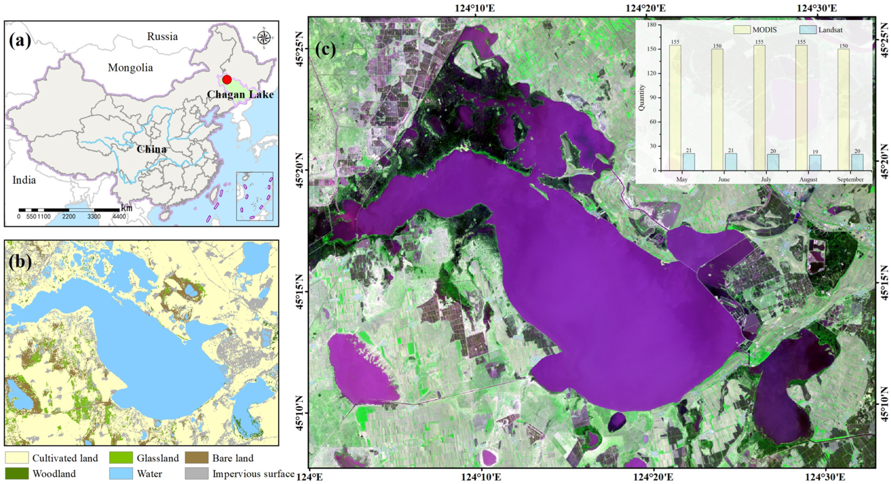
2.1. Study Area

As the seventh-largest freshwater lake in China, Chagan Lake is also the largest natural lake in Jilin Province. The geographical location of Chagan Lake is 124°03′ E–124°34′ E, 45°09′ N–45°30′ N. It is located in Qian Gorlos Mongolian Autonomous County in the northwest of Jilin Province, China. The surface of Chagan Lake is long and narrow, extending from southeast to northwest (Figure 1). The Chagan Lake region features a semi-arid temperate continental monsoon climate, marked by cold winters, hot summers, and mild spring and autumn seasons. The lake area covers 345 km², with a water storage capacity of 700 million m³ and an average water depth of 2.5 m [41]. Precipitation in Chagan Lake is mainly concentrated from July to September, with an average annual precipitation of 415.4 mm, an evaporation of 964 mm, an average temperature of 4.5 °C, and a wind speed of 3.9 m/s [42,43].

Chagan Lake is an important ecosystem and serves as a national nature reserve for inland wetlands and aquatic ecosystems, rich in natural resources. The ice period of Chagan Lake lasts for 4 months, beginning in November each winter and ending in late March of the following year [44,45]. Under the context of global climate change, lake-ice phenology serves as an effective indicator for monitoring the impacts of climate change on the lake and its surrounding environment [46]. Chagan Lake is not only a renowned fishery and reed production base but is also rich in oil and natural gas resources. However, the discharge of large volumes of water from newly constructed saline irrigation areas into Chagan Lake has led to deteriorating water quality and increased eutrophication, posing a threat to the lake’s ecological security and the sustainability of its ecological products. Therefore, high-resolution spatial and temporal remote sensing data are essential to provide robust data support for lake-ice phenology and water-quality monitoring, as well as other applications.

2.2. Data Sources

Landsat 8 is the seventh orbiting satellite in the Landsat series, launched in 2013 through a partnership between NASA and the USGS. The Enhanced Thematic Mapper (ETM+) and the Operational Land Imager (OLI) sensors aboard Landsat satellites can collect data in 15 m panchromatic and 30 m multispectral bands across 185 km-wide strips, with a spatial resolution of 30 m. This resolution is suitable for long-term surface monitoring. This study exclusively utilized Landsat multispectral data with a spatial resolution of 30 m, omitting the 15 m panchromatic band, to maintain consistency in spectral characteristics. All data have undergone USGS standard preprocessing, which, while sacrificing some spatial detail, avoids the spectral distortion that may arise from full-color sharpening, thereby making the data more suitable for long-term surface change analysis. [47].

The Moderate-Resolution Imaging Spectroradiometer (MODIS) is a sensor aboard the Terra and Aqua satellites, featuring a total of 36 bands across various spectral ranges [48]. MODIS offers three spatial resolutions: 250 m, 500 m, and 1000 m. The 250 m resolution bands (e.g., bands 1 and 2) are primarily used for observing land-surface conditions [49]. The 500 m resolution bands (e.g., bands 3–7) are suitable for observing land and cloud characteristics [50]. The 1000 m resolution bands (e.g., bands 8–36) cover a broader range of observations, including ocean watercolor, atmospheric water vapor, and surface temperature. However, MODIS has a daily revisit frequency, providing high coverage and high temporal resolution, which enables multiple daily observations of the Earth’s surface, ranging from global atmospheric monitoring to detailed analysis of surface dynamic changes.

Landsat images feature high spatial resolution but low temporal resolution, whereas MODIS images exhibit high temporal resolution yet low spatial resolution. Therefore, Landsat and MODIS images can complement each other through their respective strengths in spatiotemporal data fusion. This study is based on the Google Earth Engine (GEE) platform and employs a multi-gradient cloud-cover screening strategy to systematically acquire Landsat 8 and MODIS data for the growing season (May to September) from 2018 to 2023. Specifically, the data were divided into three cloud-cover gradients: clear-sky images with cloud cover <10% (62.3%), partially cloudy images with cloud cover between 10% and 30% (24.1%), and mostly cloudy images with cloud cover between 30% and 50% (13.6%). Additionally, concurrent Landsat 9 imagery was used as independent validation data to systematically evaluate the ESTARFM fusion results. This stratified sampling design not only ensures the quality of the foundational dataset but also enables a quantitative analysis of the impact of varying cloud-cover conditions on fusion accuracy.

Land-use data are derived from the China Multi-period Land-Use Remote Sensing Monitoring Database, which was released by the team led by Xu Xinliang at the Institute of Geographic Sciences and Natural Resources Research, Chinese Academy of Sciences (http://www.resdc.cn). These data were generated based on the interpretation of Landsat satellite images and are suitable for land-use/land-cover change analysis at both regional and national scales, with a spatial resolution of 30 m × 30 m. This study extracted six land-use types from remote sensing products for 2020: cultivated land, woodland, grassland, water, bare land, and impervious surfaces. These types were used as the foundational data for land-use classification. Historical data comparison and verification show that the main land-use types in the study area have remained stable over the long term, with no large-scale changes occurring. To account for minor local changes, spatial buffer zones were established to ensure that the potential impact of data timeliness on the study results remained within an acceptable range.

2.3. Data Processing

In this research, the primary focus was on processing data from May to September for the years 2018 to 2023. The MODIS data were resampled to a 30 m resolution using the bilinear interpolation method in the Reproject Raster Batch tool (raster batch processing) in ENVI 5.3. The resampled MODIS data were then projected to match the Landsat data source. Using the Subset Data from the Shapefile Batch tool, both datasets were clipped to the same spatial extent, resulting in a pair of remote sensing images with a spatial resolution of 30 m and dimensions of 1456 × 1186 pixels. These image pairs were used for both model input and accuracy evaluation. In this study, a total of 14 pairs of cloud-free MODIS and Landsat images were selected, as presented in

Table 1. Remote sensing data types and acquisition date (MODIS and Landsat images were selected for the same date to ensure temporal consistency).

Image ID	Data	Image ID	Data
1	5 May 2018	8	2 September 2021
2	21 May 2018	9	16 May 2022
3	6 June 2018	10	17 June 2022
4	9 August 2018	11	20 August 2022
5	10 September 2018	12	5 September 2022
6	24 May 2019	13	21 September 2022
7	13 May 2021	14	4 June 2023

.

The MODIS and Landsat images each consist of six bands, with the parameters of each band detailed in

Table 2. The information of the corresponding bands of Landsat and MODIS.

Band	Landsat	Bandwidth (nm)	MODIS	Bandwidth (nm)
Red	Band 1	0.630–0.680	Band 1	0.620–0.670
Near Infrared (NIR)	Band 2	0.845–0.885	Band 2	0.841–0.876
Blue	Band 3	0.450–0.515	Band 3	0.459–0.479
Green	Band 4	0.525–0.600	Band 4	0.545–0.565
Shortwave Infrared 1 (SWIR1)	Band 6	1.560–1.660	Band 6	1.628–1.652
Shortwave Infrared 2 (SWIR2)	Band 7	2.100–2.300	Band 7	2.105–2.155

. To reconcile the band-order differences between Landsat and the original MODIS images, the band order of the Landsat images was adjusted to align with that of the MODIS images in this study.

3. Method

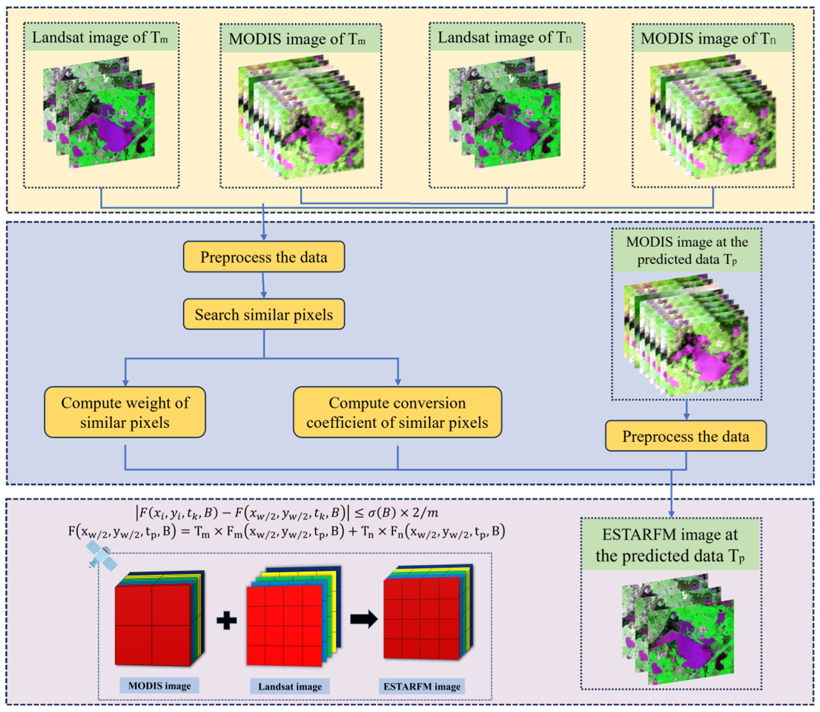
3.1. Analysis of the ESTARFM Algorithm

To generate high-spatiotemporal-resolution images of Chagan Lake, this study employs the Enhanced Spatiotemporal Adaptive Reflection Fusion Model (ESTARFM). Figure 2 illustrates the flowchart of the ESTARFM algorithm. The model requires two pairs of images as input: (1) images with low spatial resolution but high temporal resolution, and (2) images of the same reference data with high spatial resolution but low temporal resolution. Additionally, an image of the predicted data with low spatial but high temporal resolution is required to generate the high-spatial-resolution image of the predicted data. Specifically, two sets of paired MODIS and Landsat images corresponding to the same reference data, along with a MODIS image of the predicted data, are fused to generate a high-spatial-resolution image of the predicted data. The fused image is then compared and analyzed with the actual image.

The main idea of ESTARFM is to obtain the reflectance of the predicted data based on the spectral, temporal, and spatial information of the input images [19], It aims to leverage the correlation between multiple data sources for data fusion while minimizing systematic bias. The ESTARFM algorithm consists of four main steps: selecting similar neighboring pixels, calculating the weights of these pixels, determining the conversion coefficient, and estimating the reflectance of the center pixel [51,52].

1. Selection of similar neighboring pixels: Calculate the reflectance difference between neighboring pixels and the center pixel in the high-resolution image, and use a threshold value to identify similar pixel points.

$$\left|F\left(x_i,y_i,t_k,B\right)-F\left(x_{w/2},y_{w/2},t_k,B\right)\right|\le \sigma \left(B\right)\times 2/m$$

(1)

where $F\left(x_i,y_i,t_k,B\right)$ represents the fine-resolution reflectance of the neighboring pixels at the base data $\left(t_k\right)$; i denotes the pixel index within the moving window $\left(iϵ \left[1,m\right]\right)$; m is the total number of pixels in the window; k represents the time index; w represents the size of the moving window; $F \left(x_{w/2},y_{w/2},t_k,B\right)$ represents the fine-resolution reflectance of the center pixel at the base data; $\left(t_k\right), \sigma \left(B\right)$ denotes the standard deviation of the reflectance of band B.

2. Calculate the weights of similar pixels: The weight W_i is calculated based on both the positional proximity of similar pixels to the center pixel and their spectral similarity between fine-resolution and coarse-resolution pixels. Specifically, greater similarity and closer proximity result in a higher weight for the similar pixel.

3. Calculate the conversion factor: A linear regression model is employed to select fine-resolution and coarse-resolution reflectance data with similar characteristics within the same coarse-resolution pixels, thereby calculating the conversion factor.

4. Estimate the reflectance of the center pixel: The model dynamically weights and merges observation data from two reference points ($t_m$ and $t_n$), where the temporal weight reflects the time distance from the prediction point ($t_p$), and the spatial weight reflects the spectral similarity of neighboring pixels. The final output retains both spatial details and temporal variability characteristics. The formula for predicting the fine resolution reflectance at time t_p is:

$$F\left(x_{w/2},y_{w/2},t_p,B\right)=T_m\times F_m\left(x_{w/2},y_{w/2},t_p,B\right)+T_n\times F_n\left(x_{w/2},y_{w/2},t_p,B\right)$$

(2)

where $T_m=\left|t_p-t_n\right|/\left(\left|t_p-t_m\right|+\left|t_p-t_n\right|\right)$, $T_n=1-T_m$, reflects the degree of temporal proximity between the predicted time t_p and the reference times t_m and t_n. $F\left(x_{w/2}, y_{w/2},t_p,B\right)$ represents the fused reflectance value at $\left(x_{w/2}, y_{w/2}\right),t_p,$ and band B; $F_m\left(x_{w/2}, y_{w/2},t_p,B\right), F_n\left(x_{w/2}, y_{w/2},t_p,B\right)$ represent the predicted reflectance values of t_m and t_n at the reference time, respectively.

3.2. Fusion Result Accuracy Evaluation Index

The Normalized Difference Vegetation Index (NDVI, Equation (3)) is one of the best indicators of vegetation growth status and cover, defined as the difference between red and near-infrared reflectance [53]. The Normalized Difference Water Index (NDWI, Equation (4)) is a composite of climatic variables and hydrological factors, used to estimate vegetation liquid water content in spatially distributed remote sensing calculations [54]. Values ranged from −1 to 1.

$$NDVI={\displaystyle \frac{\left(NIR-\mathrm{Re}d\right)}{\left(NIR+\mathrm{Re}d\right)}}$$

(3)

$$NDWI={\displaystyle \frac{\left(Green-NIR\right)}{\left(Green+NIR\right)}}$$

(4)

where NIR, Red, and Green represent the reflectance in bands 1, 2, and 4 for Landsat and ESTARFM, respectively.

We evaluated the accuracy of the ESTARFM using the coefficient of determination (R², Equation (5)), Root Mean Square Error (RMSE, Equation (6)), and Mean Absolute Error (MAE, Equation (7)). The coefficient of determination (R²) is a measure of the goodness-of-fit of the regression function between observed and predicted data. The Root Mean Square Error (RMSE) is a measure of the deviation between the observed and true values and is commonly used to quantify the difference between predicted and actual values. Mean Absolute Error (MAE) is a measure of the difference between predicted and true values. RMSE is more sensitive to large errors and is suitable for assessing the impact of outliers, yet it amplifies these errors. MAE is more robust and reflects the average error, though it ignores directionality. In ESTARFM, RMSE is suitable for scenarios requiring maximum error control, whereas MAE is more suitable for assessing overall fusion quality. Lower RMSE and MAE values indicate that the predicted values are closer to the actual values, suggesting better model fusion performance.

$$R^2={\displaystyle \frac{{\displaystyle {\sum }_{i=1}^N{\left(x_i-\overline{y}\right)}^2}}{{\displaystyle {\sum }_{i=1}^N{\left(y_i-\overline{y}\right)}^2}}}$$

(5)

$$RMSE=\sqrt{{\displaystyle \frac{{\displaystyle {\sum }_{i=1}^N{\left(x_i-y_i\right)}^2}}{N}}}$$

(6)

$$MAE={\displaystyle \frac{{\displaystyle {\sum }_{i=1}^N\left|x_i-y_i\right|}}{n}}$$

(7)

where N denotes the sum of pixels,$x_i$,${ y}_i$ and $\overline{y}$ represent the surface reflectance value and the mean value of the i-th pixel in the predicted image and the real image, respectively.

4. Results

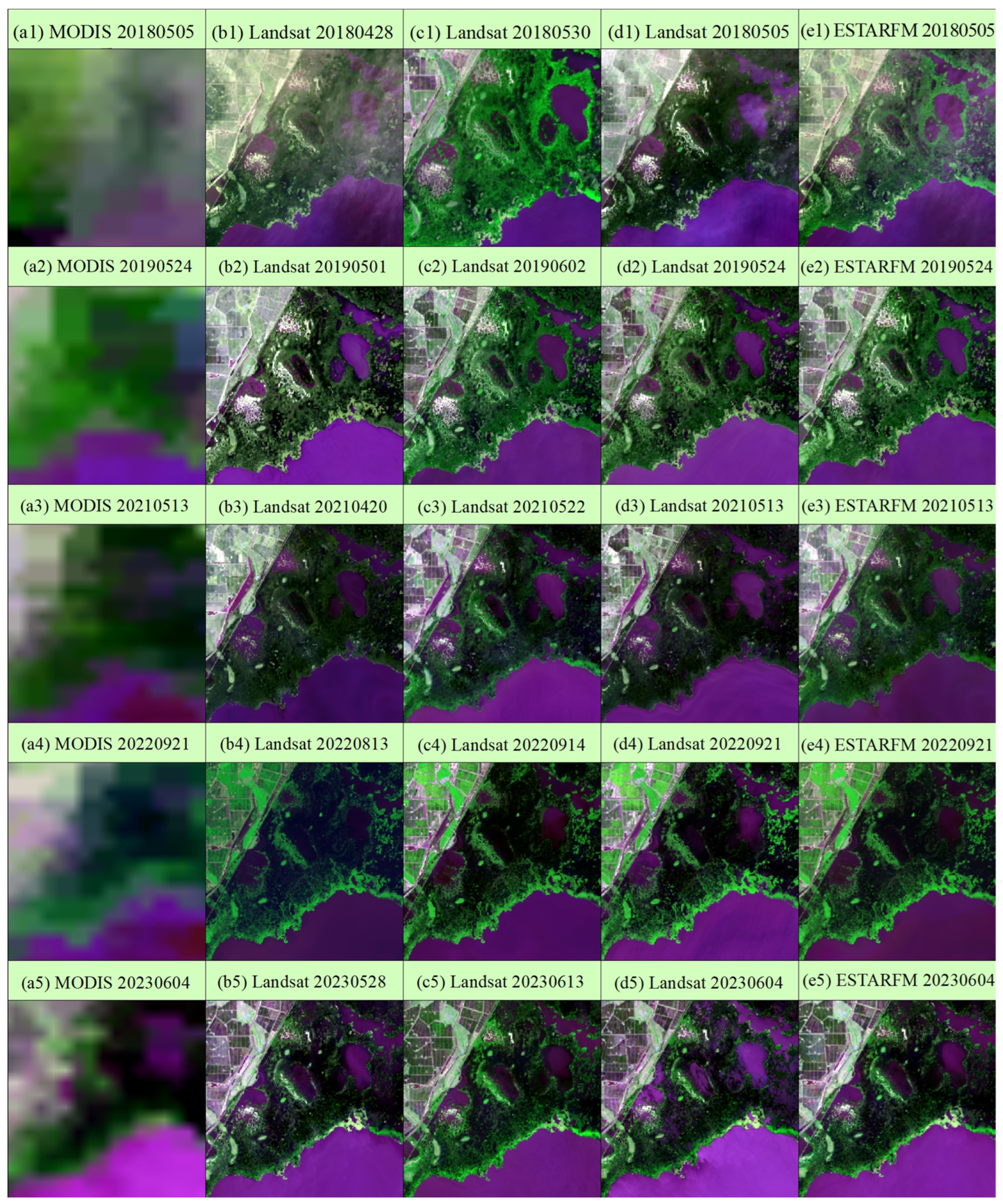
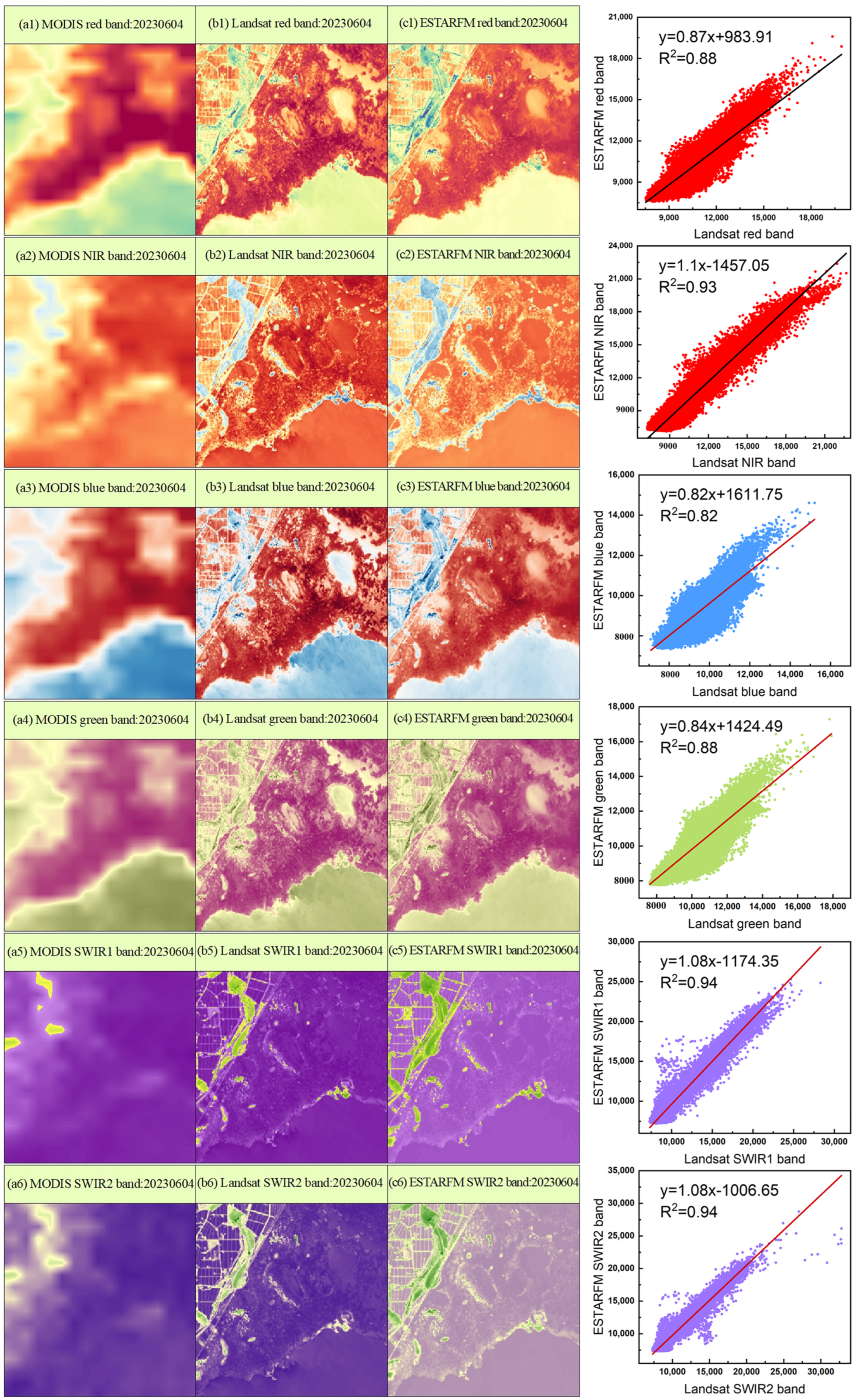
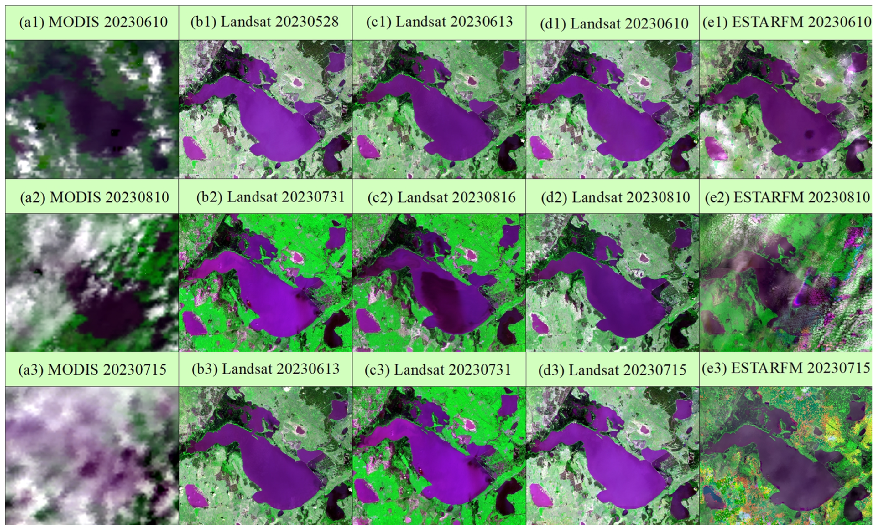
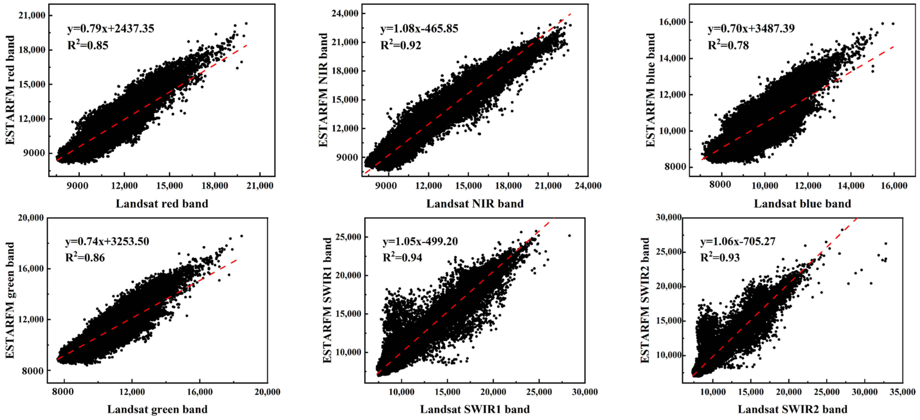
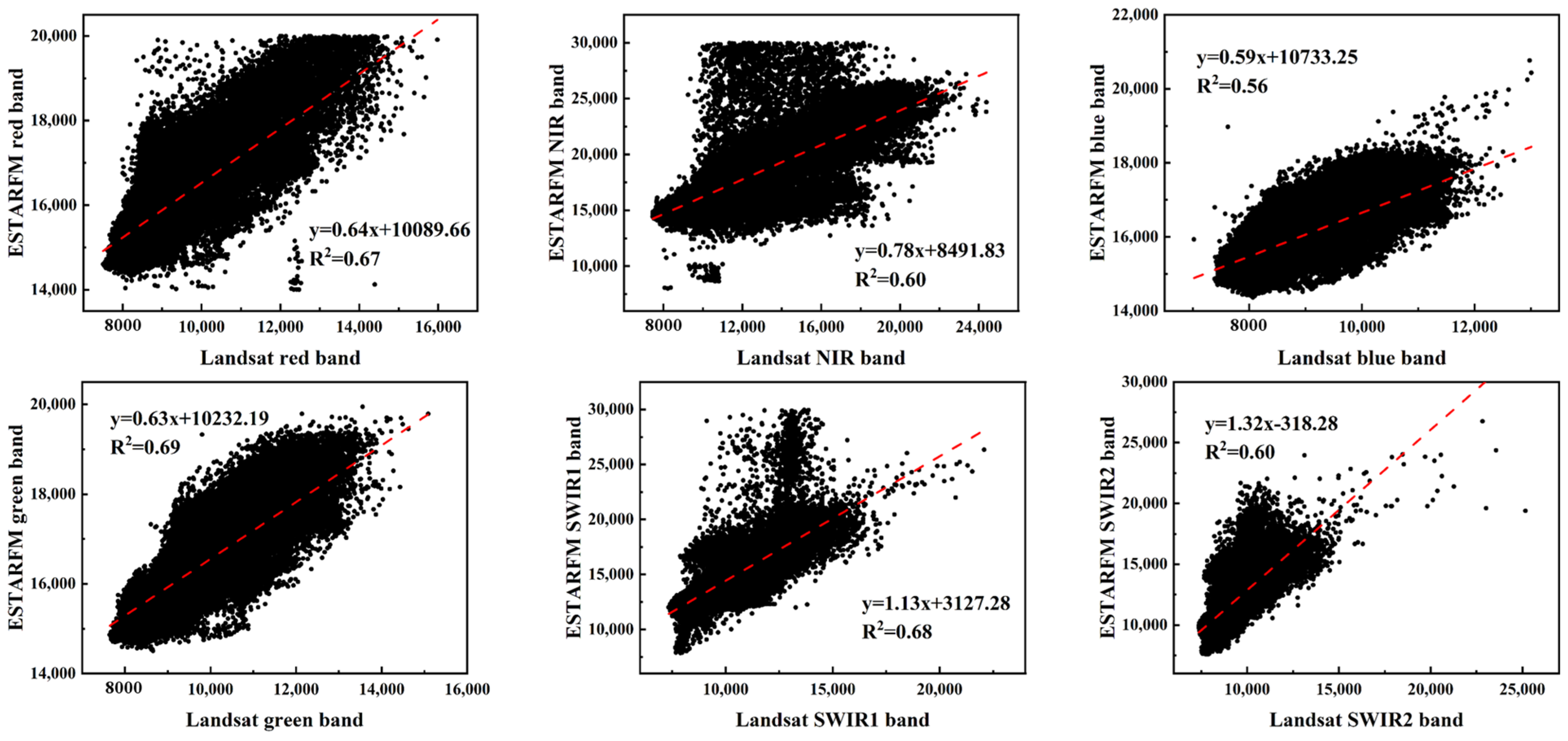
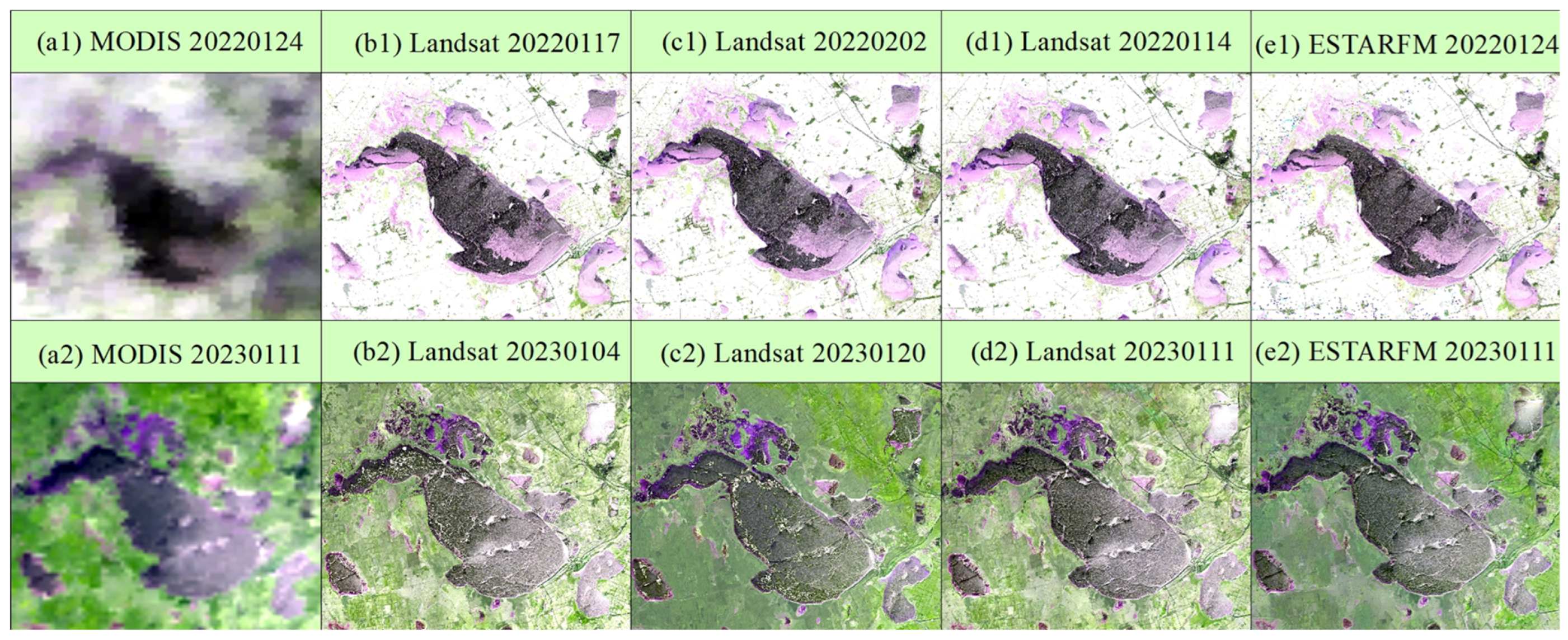
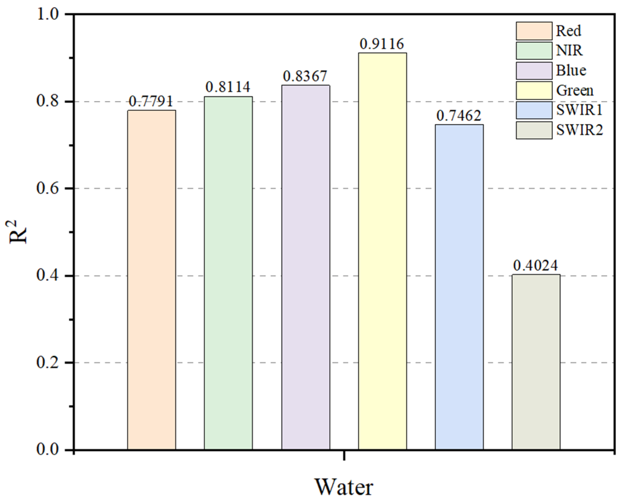
4.1. Accuracy Evaluation of Data Fusion

By merging the two most recent pairs of Landsat and MODIS image data and one MODIS image from the predicted date, a Landsat spatial-resolution composite image was generated (Figure 3). The 5 May 2018 ESTARFM image was fused using the two pairs of Landsat and MODIS image data (from 28 April and 30 May 2018) and one set of MODIS image data for 5 May 2018. The fusion effect was evaluated by comparing the fused image with the original Landsat-9 image.

The results show that through the fusion process of the ESTARFM, the obtained images are visually consistent and closely resemble the actual observation images. This result shows that the ESTARFM can effectively fuse the remote sensing data from different sensors to produce composite images with high spatial and temporal resolution that are consistent with the actual observations. Moreover, we conducted a comparative analysis of the fusion performance of the ESTARFM, FSDAF, and SFSDAF models (Figure 4). Our research revealed that, while the overall accuracy of these three models is comparable, ESTARFM exhibits superior performance in several key aspects. This model employs a dual-phase input strategy, enabling it to more accurately simulate nonlinear changes on the ground surface. Its local similarity pixel-weighting algorithm excels at preserving spatial details on heterogeneous ground surfaces, thereby avoiding the blurring of small-scale features caused by spectral unmixing in FSDAF and the artificial texture noise introduced by sharpening in SFSDAF. Leveraging these advantages, this study selected ESTARFM for an in-depth analysis.

To achieve more accurate results, this study selected images from June 4 as typical phases for the detailed analysis of six bands, primarily because they are representative: this date falls in the middle of the Landsat image acquisition cycle (with an 8-day interval between images), thereby fully meeting the ESTARFM’s optimal requirements for temporal consistency. While analyses of other dates also demonstrated high correlation (with R² values remaining above 0.80), images taken in early June had two significant advantages: first, vegetation was in a stable growth period at this time, with typical ground cover characteristics; second, atmospheric conditions were generally favorable during this period, thereby ensuring image quality. Selecting images from that day ensures both the reliability and representativeness of the analysis results. Figure 5 shows the correlation analysis between the real data and the ESTARFM fusion image for each band, with the coefficients of determination being 0.88, 0.93, 0.82, 0.88, 0.94, 0.94, indicating a high degree of correlation. These results demonstrate that the ESTARFM has achieved satisfactory performance for each band.

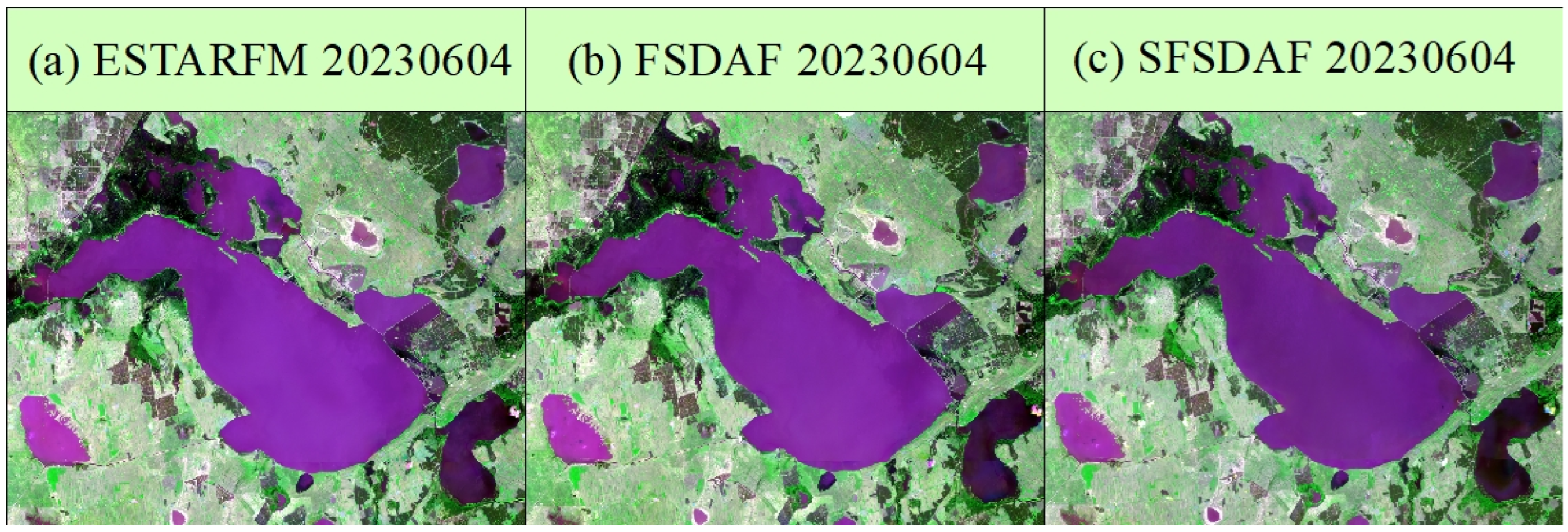
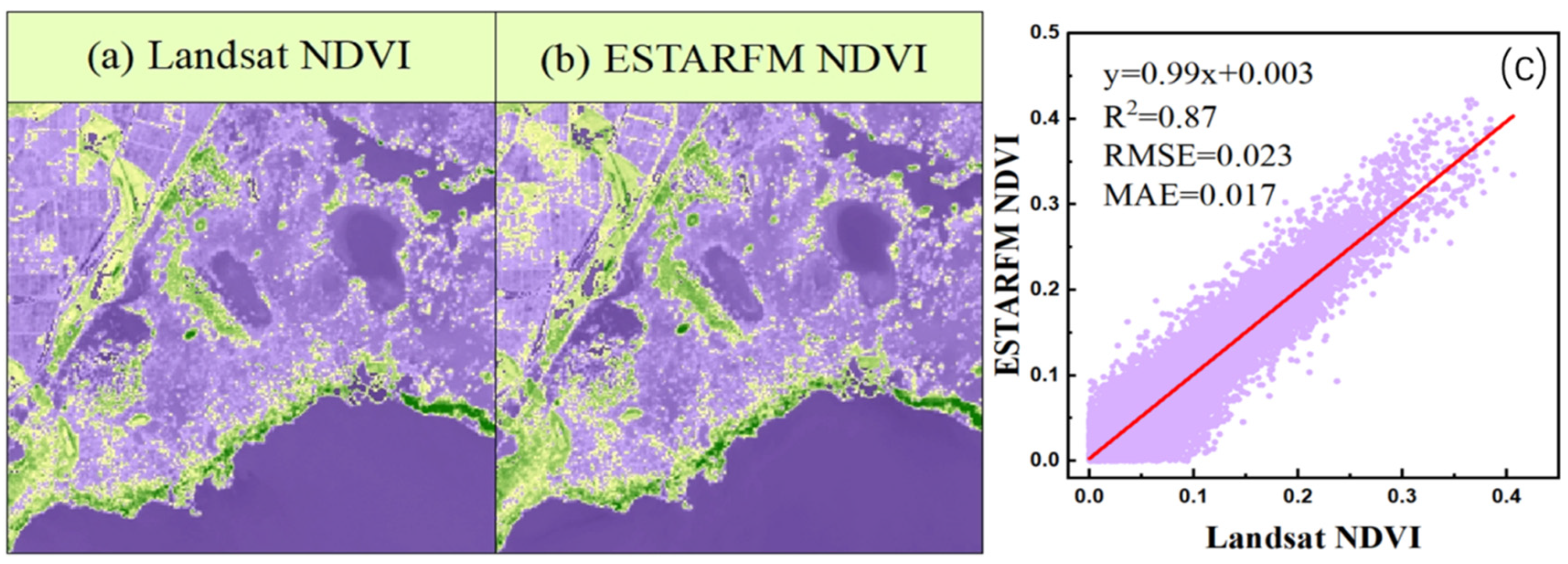
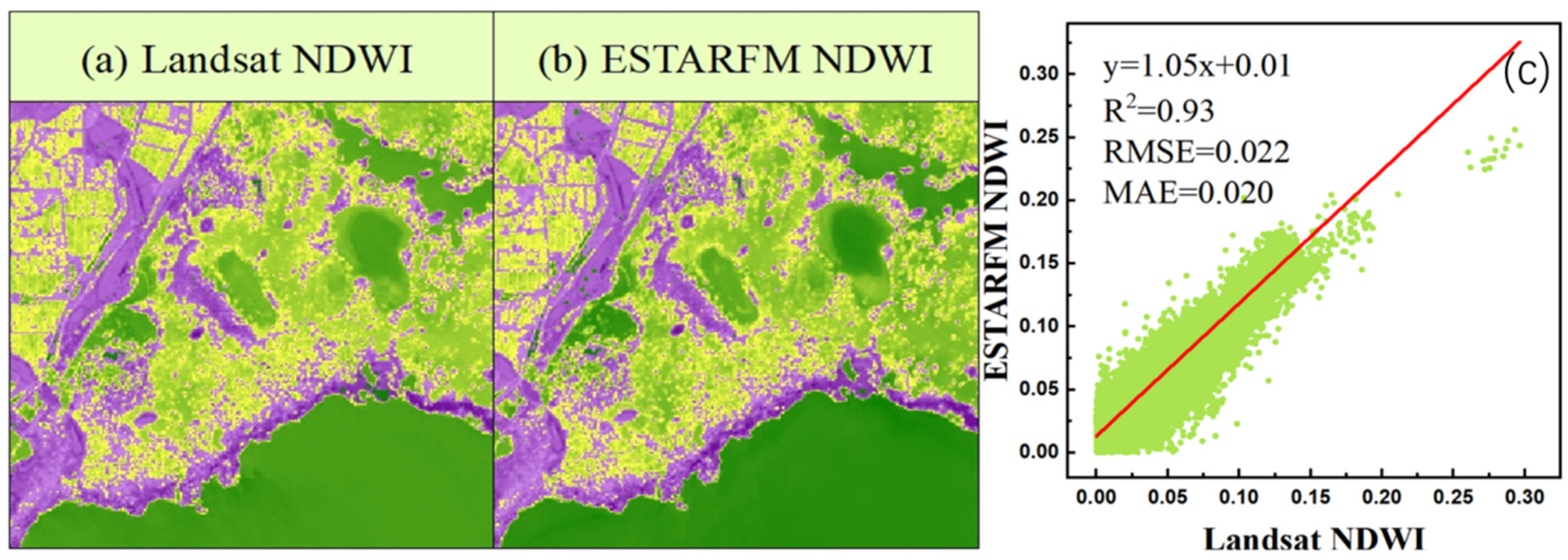
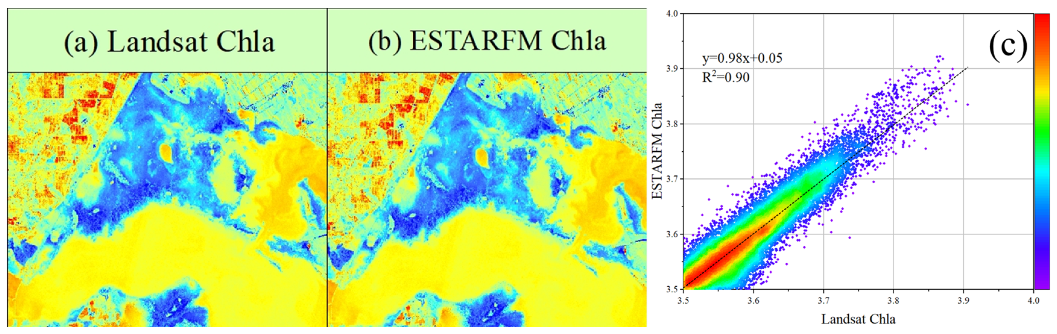
4.2. Evaluation of the Effectiveness of Post-Fusion Imaging Applications

In the study area, 50,000 sample points were selected, and the NDVI and NDWI values of the predicted ESTARFM images were compared with those of the actual Landsat images using scatter plots to visually assess the discrepancies between the fused and actual NDVI and NDWI values. In this paper, the coefficient of determination (R²), Mean Absolute Error (MAE), and Root Mean Square Error (RMSE) were calculated to assess the accuracy of the ESTARFM.

Figure 6 and Figure 7 present the comparison of NDVI and NDWI values derived from Landsat real data and ESTARFM fusion results. The results indicate that the NDVI and NDWI values derived from the ESTARFM fusion results and the actual Landsat images are visually almost identical. The correlation analysis of the images shows that the coefficient of determination is 0.87 and 0.93; the MAE values of 0.017 and 0.020, along with the RMSE values are 0.023 and 0.022, demonstrating a high degree of correlation. The results demonstrate that the ESTARFM fusion results in this region exhibit high accuracy compared to the actual Landsat images. Therefore, vegetation indices and water information can be effectively extracted using the fusion results obtained from the ESTARFM.

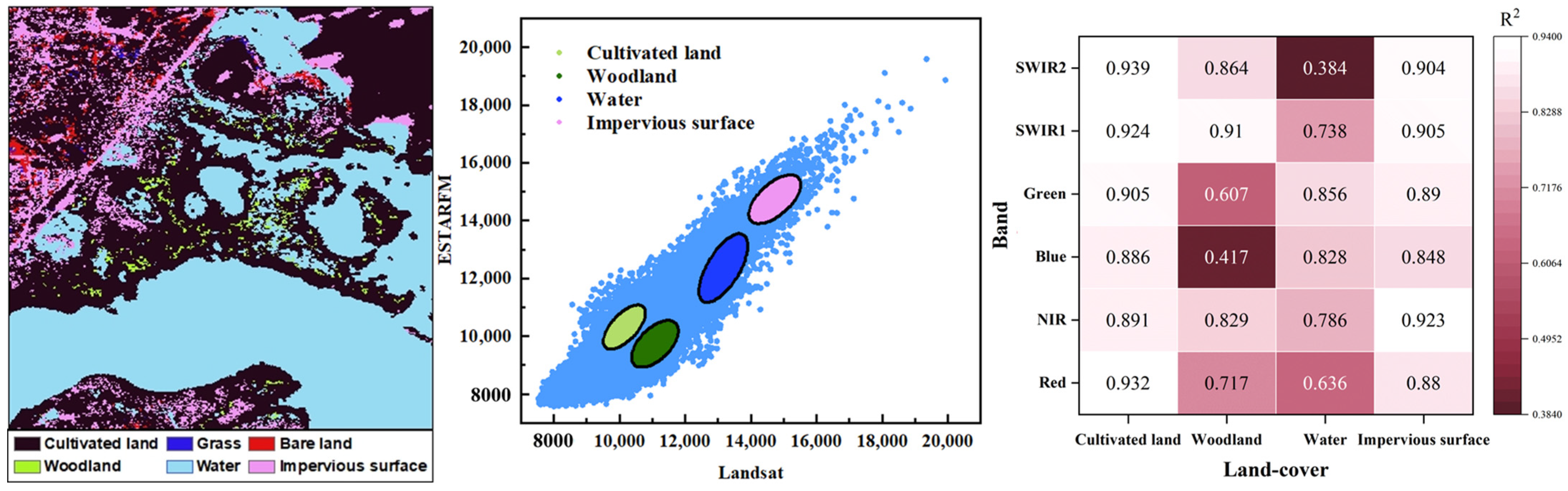
4.3. Evaluation of the Accuracy of Different Land-Cover Categories

To assess the accuracy of the ESTARFM across different land-use types, we assessed four land-use types in the fusion results for the selected region, including cropland, forested land, water, and impervious surfaces. Figure 8 shows the fusion accuracy of the four land-use types in the selected area and the cross-band fusion accuracy evaluation results of ESTARFM.

Figure 8 presents the different land-cover types in the specified area of Chagan Lake on the left, the accuracy analysis of farmland, forest land, water bodies, and impervious surfaces in the middle, and the R² values of each band for farmland, forest land, water bodies, and impervious surfaces on the right. The results indicate that most of the fused images from the ESTARFM across different bands are highly positively correlated with the actual Landsat images. However, the blue band for forest land and the SWIR2 band for water exhibit lower coefficients of determination. This may be attributed to multiple scattering by the vegetation canopy, which causes nonlinear reflection in the blue band, and to the strong absorption characteristics of water bodies in the SWIR2 band, which reduce the signal-to-noise ratio. This limitation restricts the application of fusion data in fields such as mineral identification, which require accurate SWIR2 information. Overall, the ESTARFM can effectively enhance the spatiotemporal availability of raw data. By generating high-spatiotemporal-resolution fusion images, it provides a more complete and continuous data foundation for land-use classification research, thereby significantly improving classification accuracy.

5. Discussion

5.1. The Effect of Clouds on the Fusion Effect

Few satellites are currently capable of penetrating clouds to obtain surface information, and the remote sensing images obtained are often obscured by clouds and their shadows [55,56]. This poses significant challenges for image fusion and application, particularly in regions with prolonged cloud cover, where optical remote sensing imaging is severely impacted [57]. As a result, a large number of cloud-covered pixels appear in visible remote sensing images, which substantially diminishes the continuity and effectiveness of feature observation [58,59]. The fusion accuracy was evaluated using clear-sky images with cloud cover < 10%, partly cloudy images with cloud cover between 10% and 30%, and mostly cloudy images with cloud cover between 30% and 50% as inputs to the ESTARFM, as shown in Figure 9.

The results indicate that despite the relatively short time interval of the input data, the fusion process of the ESTARFM produces images that are slightly different from the actual observed images.

To obtain an accurate comparison result, we also conducted a statistical analysis of the six bands. Comparative analysis was conducted using predicted images and actual observed images. As shown in Figure 10, the coefficient of determination (R²) for each band is greater than 0.8, even when the MODIS image contains a small amount of cloud cover. This suggests that the fused images can also be applied in other contexts. When MODIS images are covered by heavy clouds, the R² values for each band range from 0.5 to 0.7, indicating lower fusion accuracy (Figure 11). Cloud cover causes varying degrees of divergence across the bands. Consequently, under conditions of extensive cloud cover, fusion accuracy is significantly compromised.

To mitigate the impact of clouds on image-fusion accuracy, scholars both domestically and internationally have conducted extensive research on cloud removal, leading to the development of more mature cloud-removal algorithms. For example, Chen et al. [60] introduced a spatiotemporal data-fusion model for cloud removal and utilized the ESTARFM to repair cloud-covered areas in images. Gao et al. [61] applied the ATCOR2 atmospheric correction method to significantly reduce cloud and fog interference in remote sensing images. The study demonstrated that image-fusion accuracy improved from 0.58 to 0.78 after atmospheric correction. Zhou et al. [62] enhanced the sensitivity to vegetation by optimizing the vegetation–bare soil hybrid-image-element model. This optimization enabled image fusion to maintain high accuracy even under cloudy conditions and significantly improved the usability of remote sensing data in complex weather conditions. In the future, with the continuous development of cloud-removal algorithms, we will be able to utilize limited remote sensing images more effectively, significantly reducing cloud interference. When combined with spatiotemporal data-fusion models, cloud-removal technology can enhance data continuity, which is of great significance for expanding the application range of remote sensing data [63].

5.2. Reflective Properties of Water and the Use of ESTARFM

As the largest salt–alkali plain shallow water lake in Jilin Province, Chagan Lake, rich in natural resources, plays a vital role in the construction of river and lake connectivity projects in western Jilin Province and serves as a significant ecological barrier in the region. In recent years, the rapid expansion of agricultural activities and urbanization around Chagan Lake, coupled with the characteristics of “black soil” in Northeast China, has led to large amounts of soil leaching, with suspended matter and high concentrations of nutrients being discharged into Chagan Lake. This has resulted in severe eutrophication, a significant decline in the lake’s self-purification capacity, and substantial degradation of the aquatic ecological environment, thereby greatly affecting the ecological functions of Chagan Lake.

Conventional water-quality-parameter monitoring methods are often time-consuming and labor-intensive, with issues such as poor timeliness, which are not conducive to the accurate study of water-quality parameters. Moreover, water pollution can alter the optical characteristics of water bodies, leading to changes in spectral information. Traditional monitoring methods are often ineffective in capturing these changes. However, remote sensing technology can efficiently derive key water-quality parameters through the combination of multispectral bands: the blue-green band ratio is used for chlorophyll a (Chla) inversion [64], the red-blue band ratio characterizes transparency (SDD) [65], the red band is used for monitoring total suspended matter (TSM) [66], and the blue band is used for tracking lake-ice phenology changes [43]. However, the low temporal resolution of Landsat satellites and the low spatial resolution of MODIS satellites limit their ability to achieve high-frequency and high-resolution inversion of water-quality parameters. In contrast, the ESTARFM employed in this study can provide a long time series of continuous image data, facilitating more detailed and frequent monitoring. This study employs Chla as an example to validate the reflectance characteristics of the blue-green band in the fusion image against the original Landsat observation data. The results demonstrate a high degree of consistency between the two (R² = 0.90), as illustrated in Figure 12. This result not only confirms the high fidelity of the fusion algorithm in the Chla-sensitive band but also provides a robust data foundation for subsequent water-quality-parameter inversion studies using fusion data.

Lake ice is a crucial component of the cryosphere and serves as a highly sensitive indicator of climate change [67,68]. Lake-ice phenology monitoring in cold regions is crucial for understanding climate change, protecting the ecosystem, managing water resources, and predicting natural disasters [69,70,71]. However, in lake-ice phenology monitoring research, the insufficient spatiotemporal resolution of a single remote sensing data source often leads to decreased accuracy in lake-ice extraction and the misjudgment of phenological characteristics. High-spatiotemporal-resolution images generated through ESTARFM fusion can clearly present the spectral and texture characteristics of the ice–water boundary, thereby significantly improving the accuracy of visual interpretation of winter ice conditions and effectively reducing monitoring errors caused by data loss (Figure 13).

Figure 14 shows the reflectance of the water in different bands, revealing that water exhibits strong reflectance in the blue and green bands. Therefore, the ESTARFM can be employed to monitor and evaluate various water-quality parameters in the future. Additionally, it can be applied to support ecological balance and lake-ice phenology detection in Chagan Lake and other similar lakes.

5.3. Advantages and Limitations of ESTARFM

The ESTARFM offers several advantages. First, it can significantly enhance the spatial resolution of low-resolution images, thereby generating high-resolution images. Secondly, by fusing time-series images, ESTARFM can maintain temporal continuity and generate high-resolution images with multi-temporal information, which is crucial for long-term change analysis. In addition, the algorithm design of ESTARFM enables it to flexibly handle different types and temporal scales of remote sensing image data, and adapt to the image-fusion requirements under diverse environmental and geographical conditions. Especially in regions with higher heterogeneity, ESTARFM shows better applicability and accuracy, lower sensitivity to the quality of input data, and greater stability. Ultimately, the ESTARFM algorithm improves the ability to produce imagery with high-resolution temporal and spatial remotely sensed data from multiple satellite data sources, contributing to the monitoring of intra-annual surface and ecological changes at the spatial scales most relevant to human activities. ESTARFM significantly enhances the ability of traditional STARFM to process nonlinear mixed pixels by introducing a time-response conversion coefficient, yet it still has some limitations. First, when dealing with highly dynamic changes (such as sudden disasters or rapid phenological changes), its linear weighting assumption may introduce fusion bias. Although MODIS and Landsat data exhibited good linear consistency in this study, differences in band response when ESTARFM is used with other sensor combinations may further exacerbate nonlinear errors. Secondly, the ESTARFM algorithm is computationally intensive; it requires at least two pairs of high- and low-resolution images acquired on the same day, which can lead to increased computational demands. In addition, due to cloud interference, acquiring images from two high-resolution input pairs simultaneously can be challenging, thereby increasing the complexity of applying the algorithm. For scenarios with higher nonlinearity, future options include deep learning-based models (e.g., STFDCNN and DAFNet), sparse representation methods (e.g., SPSTFM), and physics–data hybrid models to overcome these limitations.

6. Conclusions

This study demonstrates the unique value of the ESTARFM in environmental monitoring for lakes. By constructing a high temporal and spatial fusion sequence of Landsat and MODIS, we have successfully overcome the technical limitations associated with the prolonged scarcity of high-resolution observation data in Chagan Lake. Multi-dimensional validation results demonstrate that the model has three significant advantages in monitoring of lake ecosystems:

• The ESTARFM achieves high-precision spectral fusion across the visible to thermal infrared bands, especially in the near-infrared and shortwave infrared bands. This capability provides a reliable basis for data acquisition in the retrieval of water parameters.
• By maintaining the high accuracy of NDVI/NDWI, the enhanced spatial resolution of ESTARFM fusion data enables a clear depiction of the micro-variations in the vegetation–water transition zone. This supplies high-precision spatiotemporal observational data for examining wetland ecological boundaries and is especially beneficial for tracking ecological responses to water-level changes.
• The ESTARFM can stably process various types of surface data, efficiently generate water-quality monitoring data with high spatial and temporal resolution, and provide reliable data support for the high-frequency monitoring of lake water quality.

References

- Zhang, L.; Weng, Q.; Shao, Z. An evaluation of monthly impervious surface dynamics by fusing Landsat and MODIS time series in the Pearl River Delta, China, from 2000 to 2015. Remote Sens. Environ. 2017, 201, 99–114. [Google Scholar]
- Zhu, X.; Leung, K.H.; Li, W.S.; Cheung, L.K. Monitoring interannual dynamics of desertification in Minqin County, China, using dense Landsat time series. Int. J. Digit. Earth 2019, 13, 886–898. [Google Scholar]
- Emelyanova, I.V.; McVicar, T.R.; Van Niel, T.G.; Li, L.T.; van Dijk, A.I.J.M. Assessing the accuracy of blending Landsat–MODIS surface reflectances in two landscapes with contrasting spatial and temporal dynamics: A framework for algorithm selection. Remote Sens. Environ. 2013, 133, 193–209. [Google Scholar]
- Sun, R.; Chen, S.; Su, H.; Mi, C.; Jin, N. The Effect of NDVI Time Series Density Derived from Spatiotemporal Fusion of Multisource Remote Sensing Data on Crop Classification Accuracy. ISPRS Int. J. Geo-Inf. 2019, 8, 502. [Google Scholar]
- Kwan, C.; Zhu, X.; Gao, F.; Chou, B.; Perez, D.; Li, J.; Shen, Y.; Koperski, K.; Marchisio, G. Assessment of Spatiotemporal Fusion Algorithms for Planet and Worldview Images. Sensors 2018, 18, 1051. [Google Scholar] [CrossRef] [PubMed]
- Wang, Q.; Atkinson, P.M. Spatio-temporal fusion for daily Sentinel-2 images. Remote Sens. Environ. 2018, 204, 31–42. [Google Scholar]
- Tian, F.; Wang, Y.; Fensholt, R.; Wang, K.; Zhang, L.; Huang, Y. Mapping and Evaluation of NDVI Trends from Synthetic Time Series Obtained by Blending Landsat and MODIS Data around a Coalfield on the Loess Plateau. Remote Sens. 2013, 5, 4255–4279. [Google Scholar]
- Battude, M.; Al Bitar, A.; Morin, D.; Cros, J.; Huc, M.; Marais Sicre, C.; Le Dantec, V.; Demarez, V. Estimating maize biomass and yield over large areas using high spatial and temporal resolution Sentinel-2 like remote sensing data. Remote Sens. Environ. 2016, 184, 668–681. [Google Scholar]
- Zou, X.; Liu, X.; Liu, M.; Liu, M.; Zhang, B. A Framework for Rice Heavy Metal Stress Monitoring Based on Phenological Phase Space and Temporal Profile Analysis. Int. J. Environ. Res. Public Health 2019, 16, 350. [Google Scholar]
- Zhang, B.; Liu, X.; Liu, M.; Meng, Y. Detection of Rice Phenological Variations under Heavy Metal Stress by Means of Blended Landsat and MODIS Image Time Series. Remote Sens. 2019, 11, 13. [Google Scholar]
- Lu, Y.; Wu, P.; Ma, X.; Li, X. Detection and prediction of land use/land cover change using spatiotemporal data fusion and the Cellular Automata–Markov model. Environ. Monit. Assess. 2019, 191, 68. [Google Scholar] [PubMed]
- Zhu, X.; Helmer, E.H.; Gao, F.; Liu, D.; Chen, J.; Lefsky, M.A. A flexible spatiotemporal method for fusing satellite images with different resolutions. Remote Sens. Environ. 2016, 172, 165–177. [Google Scholar]
- Wang, Q.; Zhang, Y.; Onojeghuo, A.O.; Zhu, X.; Atkinson, P.M. Enhancing Spatio-Temporal Fusion of MODIS and Landsat Data by Incorporating 250 m MODIS Data. IEEE J. Sel. Top. Appl. Earth Obs. Remote Sens. 2017, 10, 4116–4123. [Google Scholar]
- Li, X.; Foody, G.M.; Boyd, D.S.; Ge, Y.; Zhang, Y.; Du, Y.; Ling, F. SFSDAF: An enhanced FSDAF that incorporates sub-pixel class fraction change information for spatio-temporal image fusion. Remote Sens. Environ. 2020, 237, 111537. [Google Scholar]
- Guo, D.; Shi, W.; Hao, M.; Zhu, X. FSDAF 2.0: Improving the performance of retrieving land cover changes and preserving spatial details. Remote Sens. Environ. 2020, 248, 111973. [Google Scholar]
- Wu, P.; Shen, H.; Zhang, L.; Göttsche, F.-M. Integrated fusion of multi-scale polar-orbiting and geostationary satellite observations for the mapping of high spatial and temporal resolution land surface temperature. Remote Sens. Environ. 2015, 156, 169–181. [Google Scholar]
- Weng, Q.; Fu, P.; Gao, F. Generating daily land surface temperature at Landsat resolution by fusing Landsat and MODIS data. Remote Sens. Environ. 2014, 145, 55–67. [Google Scholar]
- Feng, G.; Masek, J.; Schwaller, M.; Hall, F. On the blending of the Landsat and MODIS surface reflectance: Predicting daily Landsat surface reflectance. IEEE Trans. Geosci. Remote Sens. 2006, 44, 2207–22181. [Google Scholar]
- Zhu, X.; Chen, J.; Gao, F.; Chen, X.; Masek, J.G. An enhanced spatial and temporal adaptive reflectance fusion model for complex heterogeneous regions. Remote Sens. Environ. 2010, 114, 2610–2623. [Google Scholar]
- Cheng, Q.; Liu, H.; Shen, H.; Wu, P.; Zhang, L. A Spatial and Temporal Nonlocal Filter-Based Data Fusion Method. IEEE Trans. Geosci. Remote Sens. 2017, 55, 4476–4488. [Google Scholar]
- Zurita-Milla, R.; Kaiser, G.; Clevers, J.G.P.W.; Schneider, W.; Schaepman, M.E. Downscaling time series of MERIS full resolution data to monitor vegetation seasonal dynamics. Remote Sens. Environ. 2009, 113, 1874–1885. [Google Scholar]
- Mingquan, W.; Zheng, N.; Changyao, W.; Chaoyang, W.; Li, W. Use of MODIS and Landsat time series data to generate high-resolution temporal synthetic Landsat data using a spatial and temporal reflectance fusion model. J. Appl. Remote Sens. 2012, 6, 063507. [Google Scholar]
- Wu, M.; Wu, C.; Huang, W.; Niu, Z.; Wang, C.; Li, W.; Hao, P. An improved high spatial and temporal data fusion approach for combining Landsat and MODIS data to generate daily synthetic Landsat imagery. Inf. Fusion 2016, 31, 14–25. [Google Scholar]
- Liao, L.; Song, J.; Wang, J.; Xiao, Z.; Wang, J. Bayesian Method for Building Frequent Landsat-Like NDVI Datasets by Integrating MODIS and Landsat NDVI. Remote Sens. 2016, 8, 452. [Google Scholar]
- Xue, J.; Leung, Y.; Fung, T. A Bayesian Data Fusion Approach to Spatio-Temporal Fusion of Remotely Sensed Images. Remote Sens. 2017, 9, 1310. [Google Scholar]
- Huang, B.; Song, H. Spatiotemporal Reflectance Fusion via Sparse Representation. IEEE Trans. Geosci. Remote Sens. 2012, 50, 3707–3716. [Google Scholar]
- Song, H.; Huang, B. Spatiotemporal Satellite Image Fusion Through One-Pair Image Learning. IEEE Trans. Geosci. Remote Sens. 2013, 51, 1883–1896. [Google Scholar]
- Xu, Y.; Huang, B.; Xu, Y.; Cao, K.; Guo, C.; Meng, D. Spatial and Temporal Image Fusion via Regularized Spatial Unmixing. IEEE Geosci. Remote Sens. Lett. 2015, 12, 1362–1366. [Google Scholar]
- Xie, D.; Zhang, J.; Zhu, X.; Pan, Y.; Liu, H.; Yuan, Z.; Yun, Y. An improved STARFM with help of an unmixing-based method to generate high spatial and temporal resolution remote sensing data in complex heterogeneous regions. Sensors 2016, 16, 207. [Google Scholar] [CrossRef]
- Chen, B.; Huang, B.; Xu, B. A hierarchical spatiotemporal adaptive fusion model using one image pair. Int. J. Digit. Earth 2017, 10, 639–655. [Google Scholar]
- Hilker, T.; Wulder, M.A.; Coops, N.C.; Linke, J.; McDermid, G.; Masek, J.G.; Gao, F.; White, J.C. A new data fusion model for high spatial- and temporal-resolution mapping of forest disturbance based on Landsat and MODIS. Remote Sens. Environ. 2009, 113, 1613–1627. [Google Scholar]
- Schmidt, M.; Lucas, R.; Bunting, P.; Verbesselt, J.; Armston, J. Multi-resolution time series imagery for forest disturbance and regrowth monitoring in Queensland, Australia. Remote Sens. Environ. 2015, 158, 156–168. [Google Scholar]
- Walker, J.J.; de Beurs, K.M.; Wynne, R.H.; Gao, F. Evaluation of Landsat and MODIS data fusion products for analysis of dryland forest phenology. Remote Sens. Environ. 2012, 117, 381–393. [Google Scholar]
- Liu, H.; Weng, Q. Enhancing temporal resolution of satellite imagery for public health studies: A case study of West Nile Virus outbreak in Los Angeles in 2007. Remote Sens. Environ. 2012, 117, 57–71. [Google Scholar]
- Shen, H.; Huang, L.; Zhang, L.; Wu, P.; Zeng, C. Long-term and fine-scale satellite monitoring of the urban heat island effect by the fusion of multi-temporal and multi-sensor remote sensed data: A 26-year case study of the city of Wuhan in China. Remote Sens. Environ. 2016, 172, 109–125. [Google Scholar]
- Zhang, F.; Zhu, X.; Liu, D. Blending MODIS and Landsat images for urban flood mapping. Int. J. Remote Sens. 2014, 35, 3237–3253. [Google Scholar]
- Dong, T.; Liu, J.; Qian, B.; Zhao, T.; Jing, Q.; Geng, X.; Wang, J.; Huffman, T.; Shang, J. Estimating winter wheat biomass by assimilating leaf area index derived from fusion of Landsat-8 and MODIS data. Int. J. Appl. Earth Obs. Geoinf. 2016, 49, 63–74. [Google Scholar]
- Wang, C.; Fan, Q.; Li, Q.; SooHoo, W.M.; Lu, L. Energy crop mapping with enhanced TM/MODIS time series in the BCAP agricultural lands. ISPRS J. Photogramm. Remote Sens. 2017, 124, 133–143. [Google Scholar]
- Liu, H.; Li, Q.; Bai, Y.; Yang, C.; Wang, J.; Zhou, Q.; Hu, S.; Shi, T.; Liao, X.; Wu, G. Improving satellite retrieval of oceanic particulate organic carbon concentrations using machine learning methods. Remote Sens. Environ. 2021, 256, 112316. [Google Scholar]
- Zhou, X.; Wang, P.; Tansey, K.; Zhang, S.; Li, H.; Tian, H. Reconstruction of time series leaf area index for improving wheat yield estimates at field scales by fusion of Sentinel-2, -3 and MODIS imagery. Comput. Electron. Agric. 2020, 177, 105692. [Google Scholar]
- Duan, H.T.; Zhang, Y.Z.; Zhan, B.; Song, K.S.; Wang, Z.M. Assessment of chlorophyll-a concentration and trophic state for Lake Chagan using Landsat TM and field spectral data. Environ. Monit. Assess. 2007, 129, 295–308. [Google Scholar] [PubMed]
- Song, K.S.; Wang, Z.M.; Blackwell, J.; Zhang, B.; Li, F.; Zhang, Y.Z.; Jiang, G.J. Water quality monitoring using Landsat Themate Mapper data with empirical algorithms in Chagan Lake, China. J. Appl. Remote Sens. 2011, 5, 1–17. [Google Scholar]
- Yang, Q.; Shi, X.; Li, W.; Song, K.; Li, Z.; Hao, X.; Xie, F.; Lin, N.; Wen, Z.; Fang, C.; et al. Fusion of Landsat 8 Operational Land Imager and Geostationary Ocean Color Imager for hourly monitoring surface morphology of lake ice with high resolution in Chagan Lake of Northeast China. Cryosphere 2023, 17, 959–975. [Google Scholar]
- Liu, X.M.; Zhang, G.X.; Zhang, J.J.; Xu, Y.J.; Wu, Y.; Wu, Y.F.; Sun, G.Z.; Chen, Y.Q.; Ma, H.B. Effects of Irrigation Discharge on Salinity of a Large Freshwater Lake: A Case Study in Chagan Lake, Northeast China. Water 2020, 12, 2112. [Google Scholar] [CrossRef]
- Hao, X.H.; Yang, Q.; Shi, X.G.; Liu, X.M.; Huang, W.F.; Chen, L.W.; Ma, Y. Fractal-Based Retrieval and Potential Driving Factors of Lake Ice Fractures of Chagan Lake, Northeast China Using Landsat Remote Sensing Images. Remote Sens. 2021, 13, 4233. [Google Scholar]
- Kropáček, J.; Maussion, F.; Chen, F.; Hoerz, S.; Hochschild, V. Analysis of ice phenology of lakes on the Tibetan Plateau from MODIS data. Cryosphere 2013, 7, 287–301. [Google Scholar]
- Wulder, M.A.; White, J.C.; Loveland, T.R.; Woodcock, C.E.; Belward, A.S.; Cohen, W.B.; Fosnight, E.A.; Shaw, J.; Masek, J.G.; Roy, D.P. The global Landsat archive: Status, consolidation, and direction. Remote Sens. Environ. 2016, 185, 271–283. [Google Scholar]
- Salomonson, V.V.; Barnes, W.L.; Maymon, P.W.; Montgomery, H.E.; Ostrow, H. MODIS—advanced facility instrument for studies of the earth as a system. IEEE Trans. Geosci. Remote Sens. 1989, 27, 145–153. [Google Scholar]
- Justice, C.O.; Giglio, L.; Korontzi, S.; Owens, J.; Morisette, J.T.; Roy, D.; Descloitres, J.; Alleaume, S.; Petitcolin, F.; Kaufman, Y. The MODIS fire products. Remote Sens. Environ. 2002, 83, 244–262. [Google Scholar]
- Prasad, K.; Bernstein, R.L. MODIS ocean and atmospheric applications using TeraScan software. In Proceedings of the OCEANS 2003 MTS/IEEE: Celebrating the Past Teaming Toward the Future, San Diego, CA, USA, 22–26 September 2003; p. 1580. [Google Scholar]
- Liu, M.; Liu, X.; Dong, X.; Zhao, B.; Zou, X.; Wu, L.; Wei, H. An Improved Spatiotemporal Data Fusion Method Using Surface Heterogeneity Information Based on ESTARFM. Remote Sens. 2020, 12, 3673. [Google Scholar]
- Yang, J.; Yao, Y.; Wei, Y.; Zhang, Y.; Jia, K.; Zhang, X.; Shang, K.; Bei, X.; Guo, X. A Robust Method for Generating High-Spatiotemporal-Resolution Surface Reflectance by Fusing MODIS and Landsat Data. Remote Sens. 2020, 12, 2312. [Google Scholar]
- Tucker, C.J. Red and photographic infrared linear combinations for monitoring vegetation. Remote Sens. Environ. 1979, 8, 127–150. [Google Scholar]
- McFeeters, S.K. The use of the normalized difference water index (NDWI) in the delineation of open water features. Int. J. Remote Sens. 1996, 17, 1425–1432. [Google Scholar]
- Zhang, Y.; Guindon, B.; Cihlar, J. An image transform to characterize and compensate for spatial variations in thin cloud contamination of Landsat images. Remote Sens. Environ. 2002, 82, 173–187. [Google Scholar]
- Zhu, Z.; Woodcock, C.E. Object-based cloud and cloud shadow detection in Landsat imagery. Remote Sens. Environ. 2012, 118, 83–94. [Google Scholar]
- Asner, G.P. Cloud cover in Landsat observations of the Brazilian Amazon. Int. J. Remote Sens. 2001, 22, 3855–3862. [Google Scholar]
- Arvidson, T.; Gasch, J.; Goward, S.N. Landsat 7’s long-term acquisition plan—An innovative approach to building a global imagery archive. Remote Sens. Environ. 2001, 78, 13–26. [Google Scholar]
- Saunders, R.W.; Kriebel, K.T. an improved method for detecting clear sky and cloudy radiances from avhrr data. Int. J. Remote Sens. 1988, 9, 123–150. [Google Scholar]
- Chen, Y.; Fan, J.; Wen, X.; Cao, W.; Wang, L. Research on Cloud Removal from Landsat TM Image based on Spatial and Temporal Data Fusion Model. Remote Sens. Technol. Appl. 2015, 30, 312–320. [Google Scholar]
- Gao, S.; Liu, X.; Song, J.; Shi, Z.; Yang, L.; Guo, L. Study on the Factors that Influencing High Spatio-temporal Resolution NDVI Fusion Accuracy in Tropical Mountainous Area. J. Geo-Inf. Sci. 2022, 24, 405–419. [Google Scholar]
- Zhou, H.; Bao, G.; Xu, Z.; Bayarsaikhan, S.; Bao, Y. Research on the Extraction of Key Phenological Metrics of Subalpine Meadow based on CO_2 Flux and Remote Sensing Fusion Data. Remote Sens. Technol. Appl. 2023, 38, 624–639. [Google Scholar]
- Shen, H.F.; Li, X.H.; Cheng, Q.; Zeng, C.; Yang, G.; Li, H.F.; Zhang, L.P. Missing Information Reconstruction of Remote Sensing Data: A Technical Review. IEEE Geosci. Remote Sens. Mag. 2015, 3, 61–85. [Google Scholar]
- Lyu, L.; Liu, G.; Shang, Y.; Wen, Z.; Hou, J.; Song, K. Characterization of dissolved organic matter (DOM) in an urbanized watershed using spectroscopic analysis. Chemosphere 2021, 277, 130210. [Google Scholar]
- Tao, H.; Song, K.; Liu, G.; Wen, Z.; Wang, Q.; Du, Y.; Lyu, L.; Du, J.; Shang, Y. Songhua River basin’s improving water quality since 2005 based on Landsat observation of water clarity. Environ. Res. 2021, 199, 111299. [Google Scholar]
- Wen, Z.; Wang, Q.; Liu, G.; Jacinthe, P.-A.; Wang, X.; Lyu, L.; Tao, H.; Ma, Y.; Duan, H.; Shang, Y.; et al. Remote sensing of total suspended matter concentration in lakes across China using Landsat images and Google Earth Engine. ISPRS J. Photogramm. Remote Sens. 2022, 187, 61–78. [Google Scholar]
- Cai, Y.; Ke, C.Q.; Li, X.; Zhang, G.; Duan, Z.; Lee, H. Variations of Lake Ice Phenology on the Tibetan Plateau From 2001 to 2017 Based on MODIS Data. J. Geophys. Res. Atmos. 2019, 124, 825–843. [Google Scholar]
- Chang-Qing, K.; An-Qi, T.; Xin, J. Variability in the ice phenology of Nam Co Lake in central Tibet from scanning multichannel microwave radiometer and special sensor microwave/imager: 1978 to 2013. J. Appl. Remote Sens. 2013, 7, 073477. [Google Scholar]
- Brown, L.C.; Duguay, C.R. The response and role of ice cover in lake-climate interactions. Prog. Phys. Geogr.-Earth Environ. 2010, 34, 671–704. [Google Scholar]
- Weber, H.; Riffler, M.; Noges, T.; Wunderle, S. Lake ice phenology from AVHRR data for European lakes: An automated two-step extraction method. Remote Sens. Environ. 2016, 174, 329–340. [Google Scholar]
- Knoll, L.B.; Sharma, S.; Denfeld, B.A.; Flaim, G.; Hori, Y.; Magnuson, J.J.; Straile, D.; Weyhenmeyer, G.A. Consequences of lake and river ice loss on cultural ecosystem services. Limnol. Oceanogr. Lett. 2019, 4, 119–131. [Google Scholar]