Assessing Extreme Precipitation in Northwest China’s Inland River Basin Under a Novel Low Radiative Forcing Scenario

Abstract

Accelerating climate change poses significant risks to water security and ecological stability in arid regions due to the increasing frequency and intensity of extreme precipitation events. As a climate-sensitive area, the inland river basin (IRB) of Northwest China—a critical water source for local ecosystems and socioeconomic activities—remains insufficiently studied in terms of future extreme precipitation dynamics. This study evaluated the spatiotemporal evolution of extreme precipitation in the IRB under a new low radiative forcing scenario (SSP1-1.9) by employing four global climate models (GCMs: GFDL-ESM4, MRI-ESM2, MIROC6, and IPSL-CM6A-LR). Eight core extreme precipitation indices were analyzed to quantify changes during the near future (NF: 2021–2050) and far future (FF: 2071–2100) periods. Our research demonstrated that all four models were capable of capturing seasonal patterns and exhibited inherent uncertainty. The annual total precipitation (PRCPTOT) in mountainous regions showed minimal variation, while desert areas were projected to experience a 2-6-fold increase in precipitation in the NF and FF. The Precipitation Intensity Index (SDII) weakened by approximately −10% in mountainous areas but strengthened by around +10% in desert regions. Most mountainous areas showed an increase in the maximum consecutive dry days (CDD), whereas desert regions exhibited extended maximum consecutive wet days (CWD). Moderate rainfall (P1025) variations primarily ranged between −5% and +20%, with greater fluctuations in desert areas. Heavy rainfall (PG25) fluctuated between −40% and +40%, reflecting stark contrasts in extreme precipitation between arid basins and mountainous zones. The maximum 1-day precipitation (Rx1day) and maximum 5-day precipitation (Rx5day) both showed significant increases, which indicated heightened risks from extreme rainfall events in the future. Moreover, the IRB region experienced increased total precipitation, enhanced rainfall intensity, more frequent alternations between drought and precipitation, more frequent moderate-to-heavy rainfall days, and higher daily precipitation extremes in both the NF and FF periods. These findings provide critical data for regional development planning and emergency response strategy formulation.

1. Introduction

Since the Industrial Revolution, anthropogenic emissions of carbon dioxide and other greenhouse gases have driven global mean temperatures approximately 1.1 °C above pre-industrial levels, fundamentally altering the Earth’s hydrological cycle [1,2,3,4]. Observational records reveal that daily precipitation variability has increased globally by 1.2% per decade since 1900. Over 75% of land areas have experienced amplified wet-dry oscillations, a trend that is particularly pronounced in Europe, Australia, and eastern North America [5]. This intensification has manifested as catastrophic extreme drought and extreme precipitation, exemplified by the 2021 Henan floods (which recorded rainfall rates of up to 201.9 mm/h) and the consecutive drought-flood oscillations experienced across North China in 2024 [6,7]. Extreme drought and precipitation caused 40 million people to be displaced and resulted in global economic losses of $550 billion in 2024.

Compared to a gradual increase in temperature, extreme precipitation exhibits nonlinear responses to warming. These responses are driven by atmospheric moistening (enhanced at approximately 7% per 1 °C according to Clausius—Clapeyron scaling) and modulated by regional circulation anomalies [8,9,10]. CMIP6 projections under the SSP5-8.5 scenario indicate that East Asia’s maximum 1-day precipitation (Rx1day) could increase by 50% by 2100, while Northwest China may paradoxically face reduced light precipitation despite intensified heavy rainfall [11]. This spatial heterogeneity stems from competing forcings: greenhouse gases amplify heavy precipitation through thermodynamic effects, whereas anthropogenic aerosols suppress convective activity in northern regions, exacerbating the “south-flood-north-drought” dipole pattern [12,13].

Compared with CMIP5, the average relative errors of GCMs within the framework of CMIP6 for extreme precipitation simulations have decreased significantly, especially in arid regions such as northwest China [14]. Emerging AI-driven techniques, such as Cycle-Consistent Generative Adversarial Networks, have effectively corrected CMIP6 precipitation biases in phenomena like atmospheric rivers, achieving approximately 30% better agreement with ERA5 reanalysis data for extreme precipitation intensity categories [15]. However, challenges remain, as an increase in precipitation index intensity may lead to variations or uncertainties in extreme precipitation across different products [16,17,18].

In China, CMIP6 simulations have robustly captured the transition from frequent light rainfall to heavy precipitation since the 1960s. Anthropogenic greenhouse gases dominate the wetting trend over the continent of Southeastern China, while the drying trend over the continent of Southwestern China is mainly attributed to anthropogenic aerosol emissions [19]. The extreme precipitation has increased in Northwest China after the 2000s, contributing to a warming-wetting trend in Northwest China [20]. The newly introduced Shared Socioeconomic Pathway SSP1-1.9—a scenario that strictly limits global temperature rise to 1.5 °C by 2100—represents a groundbreaking framework for aligning climate mitigation with sustainable development. Despite progress in CMIP6 assessments, the majority of current research has focused on SSP1-2.6, SSP2-4.5, SSP3-7.0, and SSP5-8.5 scenarios [21,22,23], neglecting the unique risks and opportunities posed by accelerated decarbonization under SSP1-1.9. In arid regions, these risks and opportunities are critical for balancing water security and achieving carbon neutrality. Northwest China, which relies heavily on the alpine snowpack (accounting for 40–60% of annual runoff) [24], exhibits heightened sensitivity to extreme precipitation under rapid warming conditions [25]. The absence of localized studies addressing these dynamics is a concern.

Building on the above context, this study selected four CMIP6 GCMs under the low radiative forcing SSP1-1.9 scenario to analyze the spatiotemporal distribution of eight extreme precipitation indices in Northwest China, characterizing future changes in extreme precipitation. The specific objectives include calibrating the four CMIP6 GCMs using the CN05.1 gridded observational dataset (derived from over 2400 national stations) from the China Meteorological Administration. We investigated changes in eight extreme precipitation indices across the near future (NF: 2021–2050) and far future (FF: 2071–2100) periods, as well as their impacts on basin-scale precipitation dynamics.

2. Materials and Methods

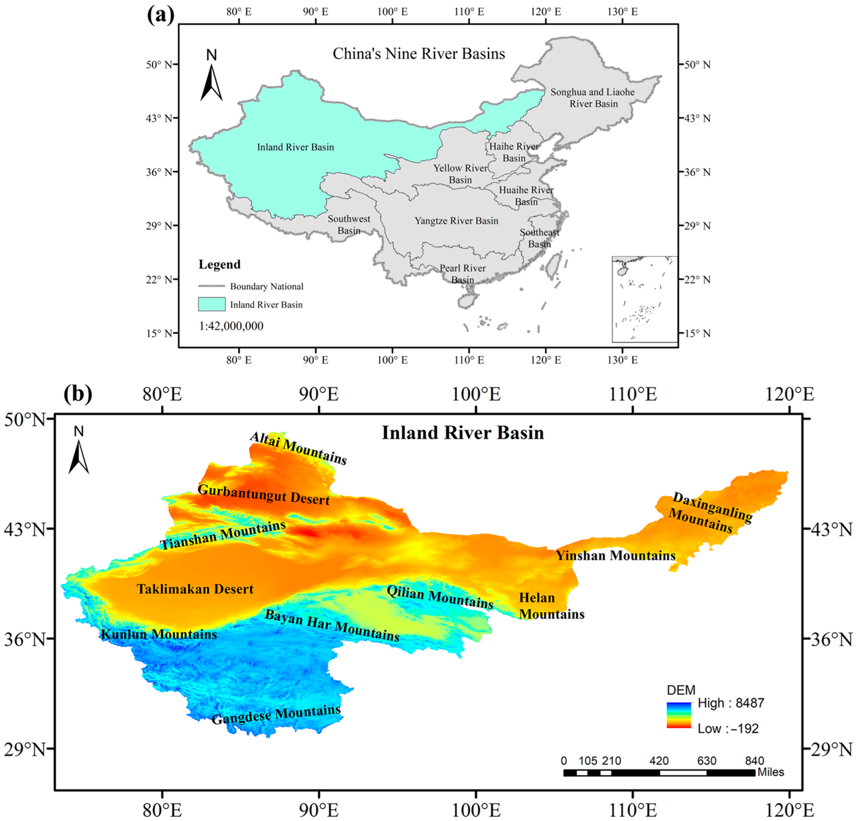
2.1. Study Area

In alignment with the guidelines of the Chinese Academy of Sciences Resource and Environment Data Center for national water resource delineation, this study categorized China into nine major river basins based on hydrological boundaries (Figure 1) [26]. The inland river basin (IRB) of Northwest China spans latitudes 29° N to 49° N and longitudes 73° E to 120° E, encompassing a total area of 3.35 million km². This region includes the Gangdese, Bayan Har, Kunlun, Tianshan, Altai, Qilian, Helan, Yinshan, and Daxinganling mountain ranges and the Taklimakan and Gurbantungut deserts. Characterized by its extreme continental remoteness and arid climate, the IRB exhibits an average annual precipitation of only 172 mm [27].

2.2. Data

This study utilized simulation data from the CMIP6 SSP1-1.9 scenario generated by four global climate models: GFDL-ESM4 (GE), MRI-ESM2 (ME), MIROC6 (MI), and IPSL-CM6A-LR (IL). These models feature spatial resolutions of 100 km and 250 km [28]. Four models (GE, ME, MI, and IL) were selected for analysis based on their resolution compatibility and data accessibility. The key model specifications are summarized in

Table 1. Basic information about the four GCMs in this study.

Abbreviation	Model ID	Country or Union	Spatial Resolution	Time Period	Type and Size
GE	GFDL-ESM4	USA	100 km × 100 km	1950–2100	Daily precipitation
ME	MRI-ESM2	Japan	100 km × 100 km	1950–2100	Daily precipitation
MI	MIROC6	Japan	250 km × 250 km	1960–2100	Daily precipitation
IL	IPSL-CM6A-LR	France	250 km × 250 km	1850–2100	Daily precipitation

. Additional details can be accessed at the World Climate Research Programme CMIP6 portal (https://www.wcrp-climate.org/wgcm-cmip (accessed on 5 July 2023)).

The precipitation data used for the evaluation were derived from the CN05.1 meteorological dataset, a high-resolution (0.25° × 0.25°) gridded daily product spanning 1961–2020. This dataset integrates observation records from more than 2400 national meteorological stations in China, mainly including seven variables: daily average temperature, maximum and minimum temperature, precipitation, humidity, wind speed, and surface evaporation. The dataset was processed using the anomaly approximation method [29]. Specifically, the methodology involves two steps: (1) interpolating the climatological mean and anomaly fields separately to minimize spatial biases, and (2) superimposing these fields to generate spatially continuous precipitation estimates. The CN05.1 dataset is widely recognized for its robustness in capturing regional climate variability and has been rigorously validated for hydrological and climatological studies in China.

To ensure consistency, all data were regridded to a standardized spatial resolution of 1° × 1°. Three time periods were analyzed: (1) baseline period (1961–2014): historical precipitation data for calibration and reference. (2) Near-future (NF) period (2021–2050): Projected precipitation data under climate scenarios. (3) Far-future (FF) period (2071–2100): Long-term projections to assess the impacts of climate change. This standardized framework ensures spatiotemporal comparability across datasets while adhering to established climate-modeling protocols.

2.3. Bias Correction

In this study, the model performance was evaluated using the percentage deviation and root mean square error (RMSE). Climate model outputs are inherently prone to systematic biases due to imperfect parameterizations and resolution limitations, which can propagate uncertainties into impact assessments [30,31,32]. To address this, we applied the Equidistant Cumulative Distribution Function (EDCDF) bias correction method to the outputs of the four selected models. The EDCDF approach minimizes distributional mismatches between modeled and observed data by adjusting the cumulative distribution functions (CDFs) of future projections based on baseline period discrepancies [33,34]. The method operates in three key steps: (1) Baseline CDF Construction: Compute the CDFs of observed and modeled precipitation during the baseline period (1961–2014) [34,35]. (2) Quantile Mapping: For the future projection period (NF and FF), the model’s CDF is calculated, and the quantile-dependent adjustment factor is determined using the baseline-period CDF differences. (3) Bias Adjustment: The derived adjustment factor is applied to the future model outputs, ensuring that the corrected values retain the model’s projected trends while aligning with the observed statistical properties. Mathematically, the EDCDF correction for a future model value $X_{MF-C}$ is expressed as:

$$X_{MF-C}=X_{MF}+F_{OH}^{-1}\left[F_{MF}\left(X_{MF}\right)\right]-F_{MH}^{-1}\left[F_{MF}\left(X_{MF}\right)\right]$$

where $X_{MF}$ and $X_{MF-C}$ are respectively the future simulation value and the deviation correction value of the model. $F_{MF}$ is the CDF in the future, $F_{OH}^{-1}$ is the inverse function of the CDF of historical observation data, while $F_{MH}^{-1}$ is the inverse function of the CDF of historical data in the model. This method preserves climate change signals while reducing systematic biases [35].

2.4. Precipitation Extreme Indices

We analyzed eight key extreme precipitation indices to evaluate the impacts of climate change in the IRB of Northwest China under the SSP1-1.9 scenario (

Table 2. Characteristics of the extreme precipitation indices used.

Number	Abbreviation	Definition	Unit
1	PRCPTOT	Total annual precipitation from days with rainfall ≥ 1 mm	mm
2	SDII	Mean daily precipitation intensity	mm/day
3	CDD	Maximum consecutive dry days (<1 mm)	days
4	CWD	Maximum consecutive wet days (≥1 mm)	days
5	P1025	Days with rainfall 10–25 mm	days
6	PG25	Days with rainfall > 25 mm	days
7	Rx1day	Maximum 1-day precipitation	mm
8	Rx5day	Maximum 5-day cumulative precipitation	mm

). These physically based metrics were selected to systematically quantify variations in precipitation intensity, duration and frequency.

3. Results

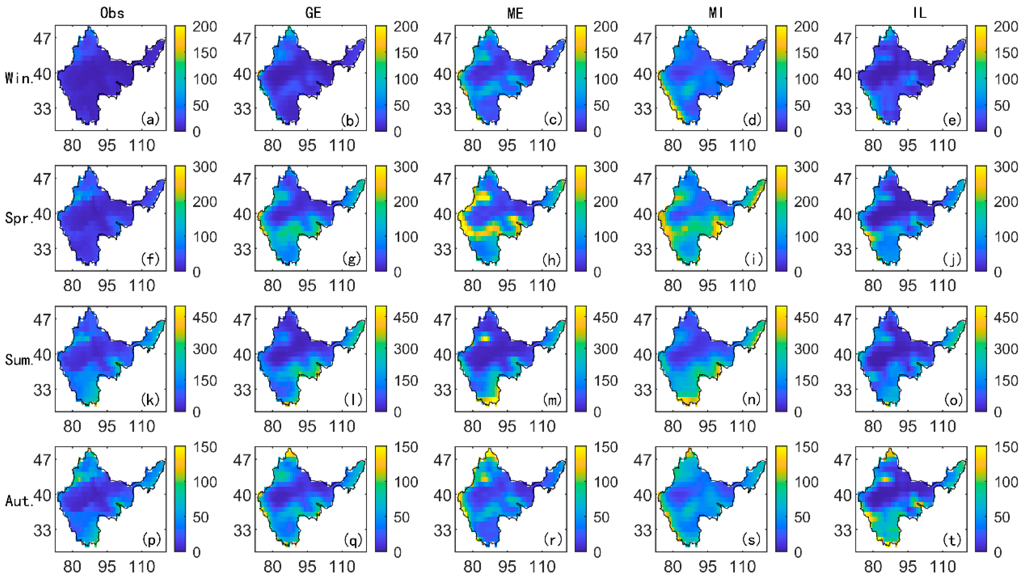
3.1. Seasonality Variability in Historical Data

This study analyzed seasonal precipitation trends in the IRB using the CN05.1 observational dataset and bias-corrected outputs from four CMIP6 models (Figure 2). Seasonal divisions were defined as follows: winter (December–February), spring (March–May), summer (June–August), and autumn (September–November). The results revealed distinct seasonal precipitation patterns, with average annual precipitation peaking at 240 mm in winter (Figure 2a–e), 500 mm in spring (Figure 2f–j), 550 mm in summer (Figure 2k–o), and 220 mm in autumn (Figure 2p–t). The IRB’s complex topography—spanning mountainous zones, oases, and arid deserts—generated strong spatial heterogeneity in precipitation distribution. Although the CMIP6 models broadly replicated the observed spatial patterns, notable seasonal biases were evident. For instance, spring simulations revealed a northwest/southwest-to-northeast/southeast precipitation gradient, diverging from observations. Summer models captured the southwest-to-northeast decline in rainfall but underestimated its intensity.

Model performance analysis highlighted that the IL model aligned most closely with historical observations, excelling at simulating extreme precipitation events during spring and summer. The GE model reproduced the winter and autumn precipitation characteristics. However, the MI model systematically overestimated rainfall, particularly in the southwestern region, across all seasons. The ME model exhibited instability, with a consistent underestimation in winter and mixed overestimation/underestimation biases in other seasons. These discrepancies may stem from challenges in parameterizing localized climatic processes under complex terrain, such as the MI model’s overamplification of orographic precipitation in southwestern mountains and the ME model’s uncertainty in simulating boundary layer dynamics in desert margins. These findings underscore the necessity of region-specific bias correction for climate models in topographically diverse regions to improve the predictive accuracy for hydrological and ecological applications.

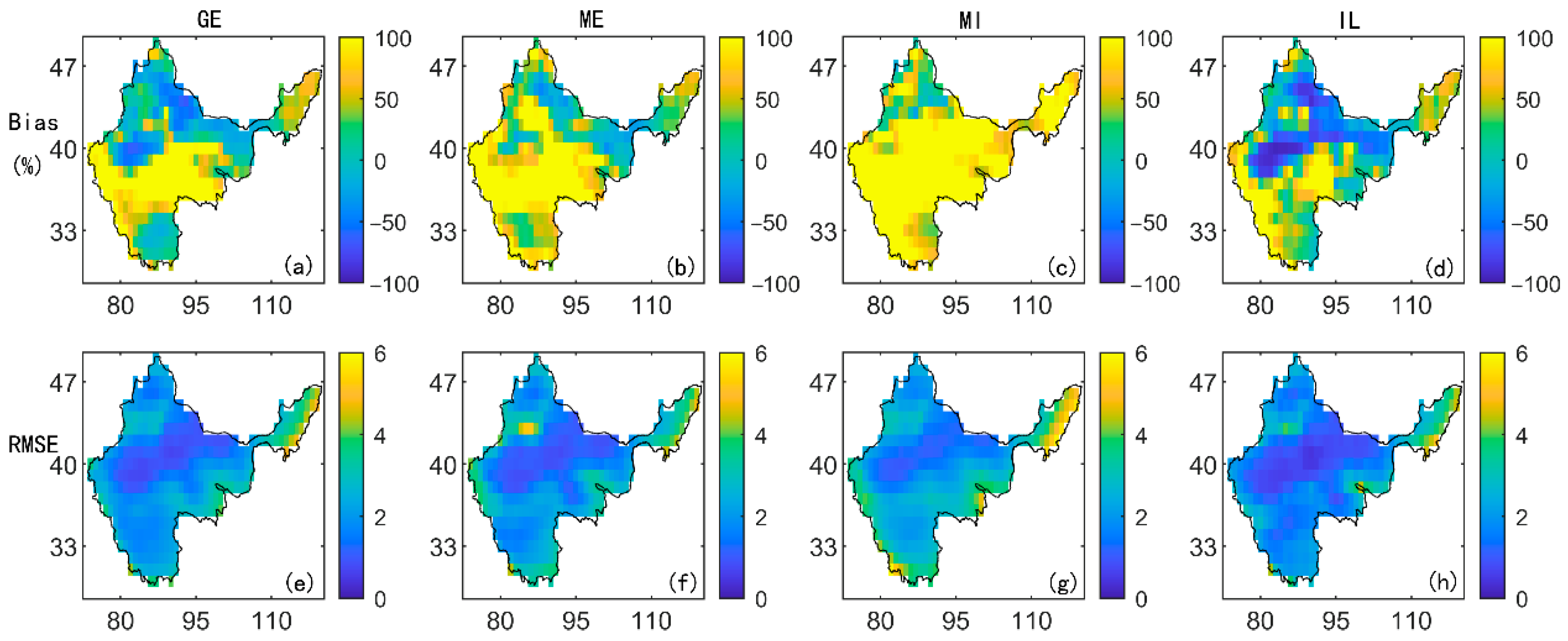
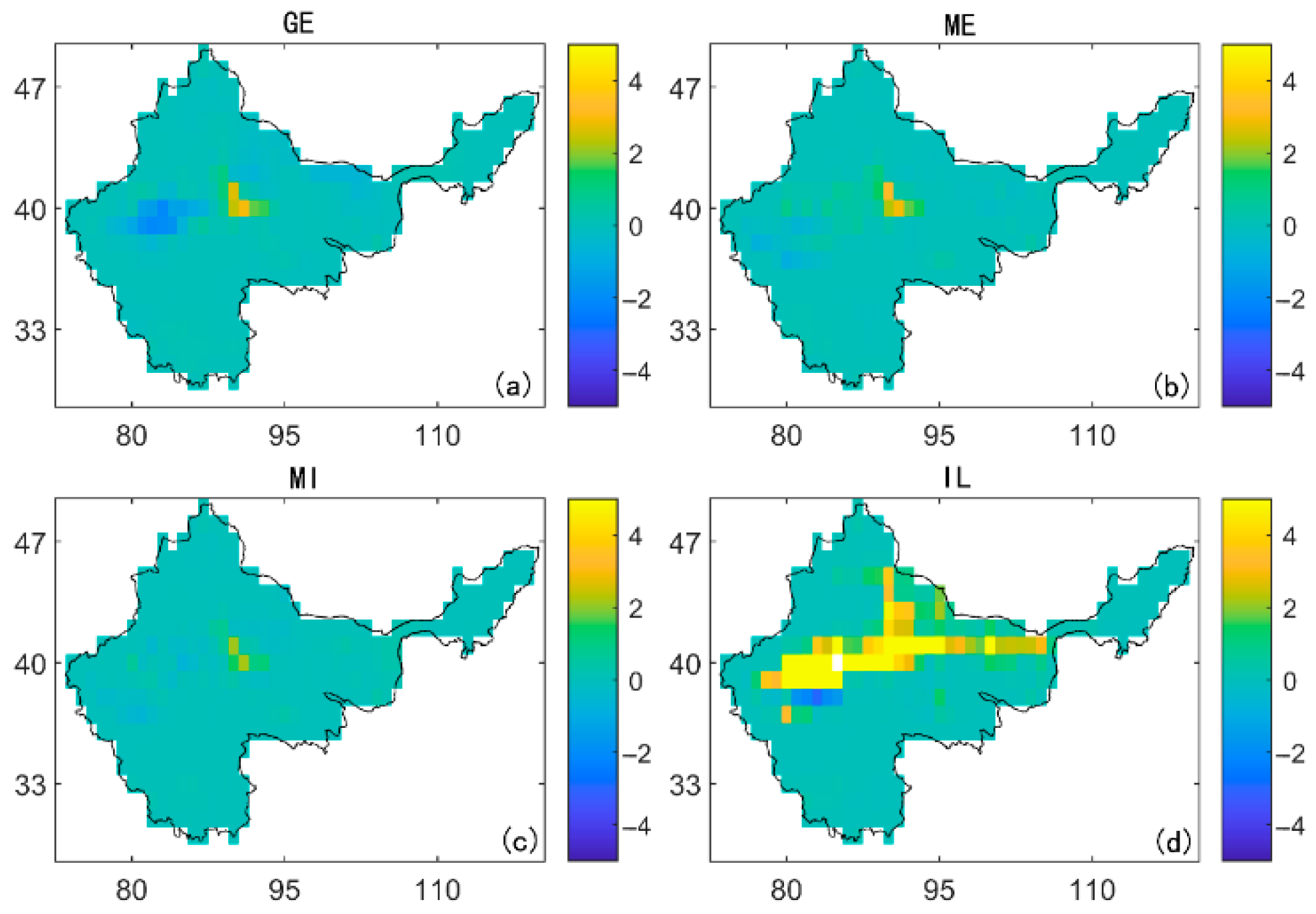
3.2. Model Evaluation and Bias Correction

The percentage bias of the selected CMIP6 GCMs and the root mean square error (RMSE) of the precipitation data relative to the observed values for each grid from 1961 to 2014 are presented in Figure 3. In Figure 3a–d, negative and positive values indicate the underestimation and overestimation of precipitation by the four GCM models compared to the observations. Most regions exhibited biases ranging from −50% to 100% in the GE, ME, and MI models, while the IL model showed a broader bias range of −50% to 75%. As shown in Figure 3a–d, biases in the northern and southern regions generally fell within −50% to 50%, with significant deviations concentrated in the southwestern and central desert areas. Among the four models, the GE model demonstrated relatively small biases, whereas the MI model displayed larger discrepancies. In Figure 3e–h, the RMSE for nearly all regions remained below 5, except for localized areas in the northeast and southwest, where values exceeded this threshold. A comparison of the RMSE across models revealed that the IL model achieved the lowest overall error, while the MI model had the highest. This indicates that the precipitation data of the IL model were more closely aligned with the observations, exhibiting lower dispersion and greater stability than those of the other models.

Figure 4 shows the deviation percentages of the four models after correction with the EDCDF compared to the observed data. Figure 4a–c shows that the deviation percentages in most regions are between −1% and 1%, and the deviation percentages in individual central regions, such as the Taklimakan Desert, are between −4% and 4%. The overall deviation correction effect of the IL plot was better, except that the deviation value of the individual areas in the middle was kept at approximately 5%.

3.3. Variability in Precipitation Extremes During Historical Events

Figure 5 illustrates the spatial distribution of extreme precipitation indices across the IRB based on observational datasets from 1961 to 2014. Figure 5a–i depicts the PRCPTOT, SDII, CDD, CWD, P1025, PG25, Rx1day, and Rx5day. The southeastern IRB and the Tianshan Mountains exhibited the highest annual precipitation (Figure 5a), contrasting sharply with the arid central desert region, which received minimal rainfall. The PRCPTOT (Figure 5b) mirrored the spatial pattern of annual precipitation, with both showing elevated totals in the southeast and northwest. A strong correlation between PRCPTOT and SDII (Figure 5c) was evident in these moisture-rich regions, whereas the central desert and Kunlun Mountains displayed weak correlations, likely due to sporadic rainfall events.

The Taklimakan Desert recorded the longest consecutive dry days (CDD > 120 days/year, Figure 5d), while the northwestern IRB experienced the shortest dry spells. The CWD was generally limited across the basin, exceeding 10 days/year only in localized areas such as the eastern Qilian Mountains, Tianshan foothills, and southern Qinghai-Tibet Plateau margins (Figure 5e). Moderate rain days (P1025) were confined to high-elevation zones, including the Tianshan, southern Gangdise, eastern Qilian, and northeastern Daxinganling Mountains (Figure 5f). Heavy rain events (PG25) were rare, occurring exclusively in the Daxinganling Mountains with an annual average of 1.5 days (Figure 5g). Both Rx1day (maximum: ~35 mm) and Rx5day (maximum: ~60 mm) exhibited similar spatial gradients, decreasing from the humid southeastern and northwestern peripheries toward the central basin (Figure 5h,i). This pattern underscored the dominant influence of orographic uplift in the mountainous regions and the rain-shadow effect in the central desert.

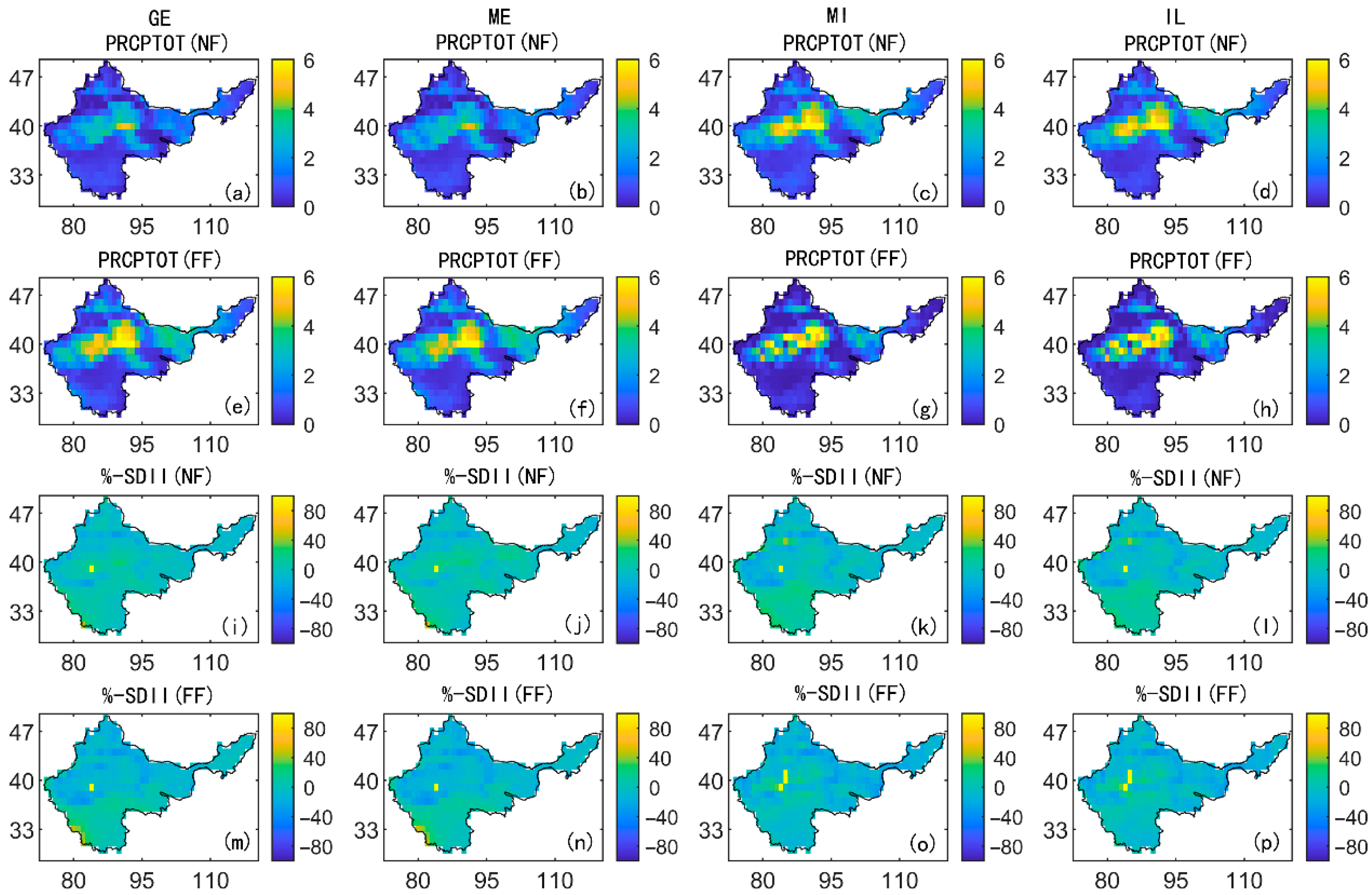
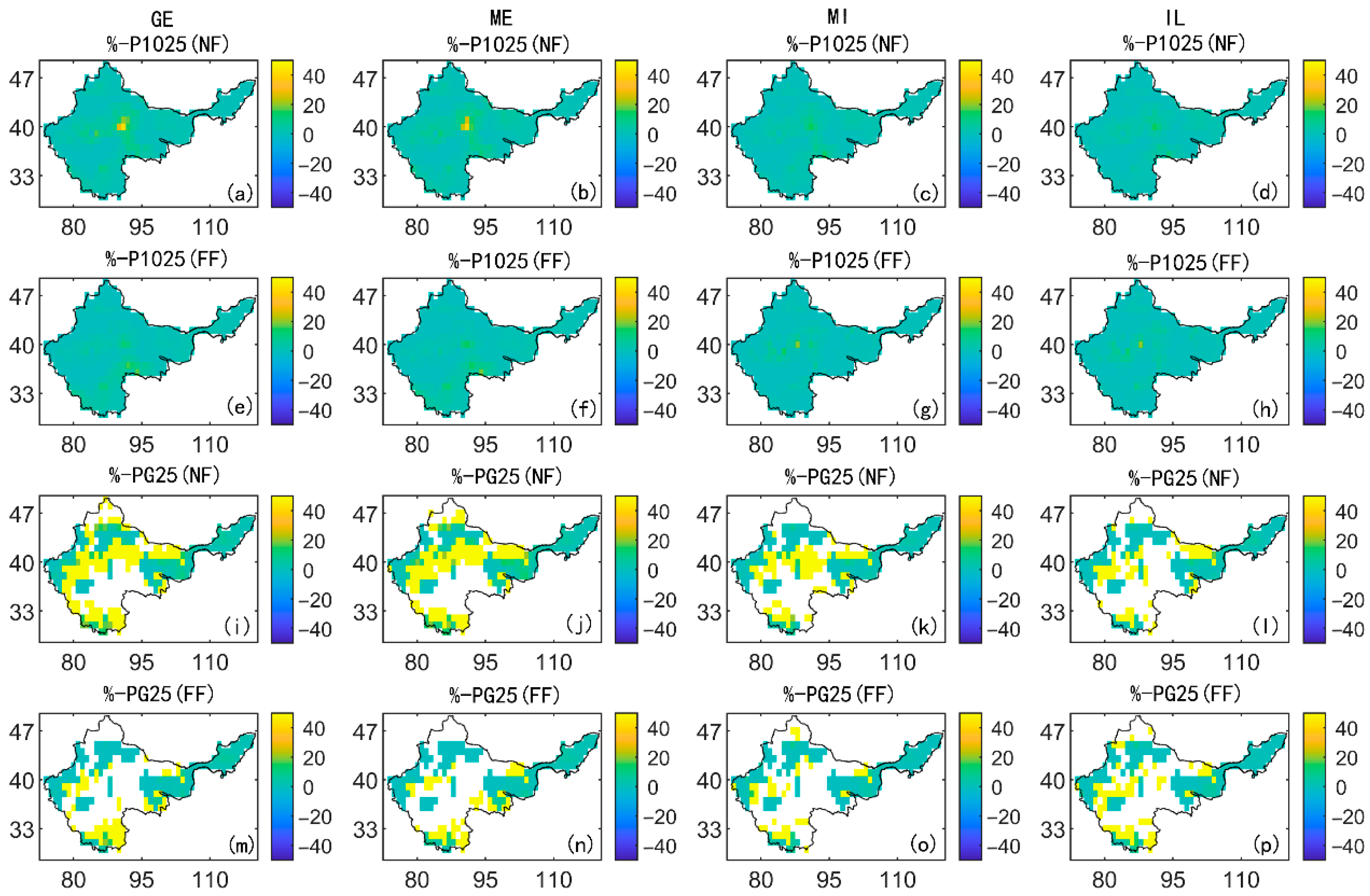
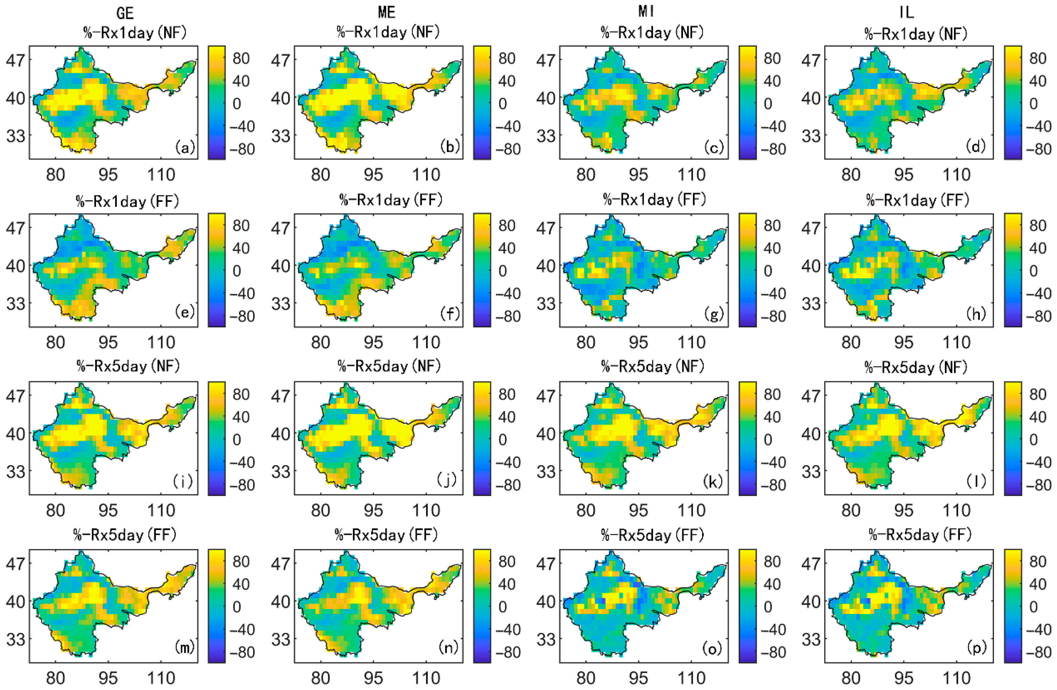
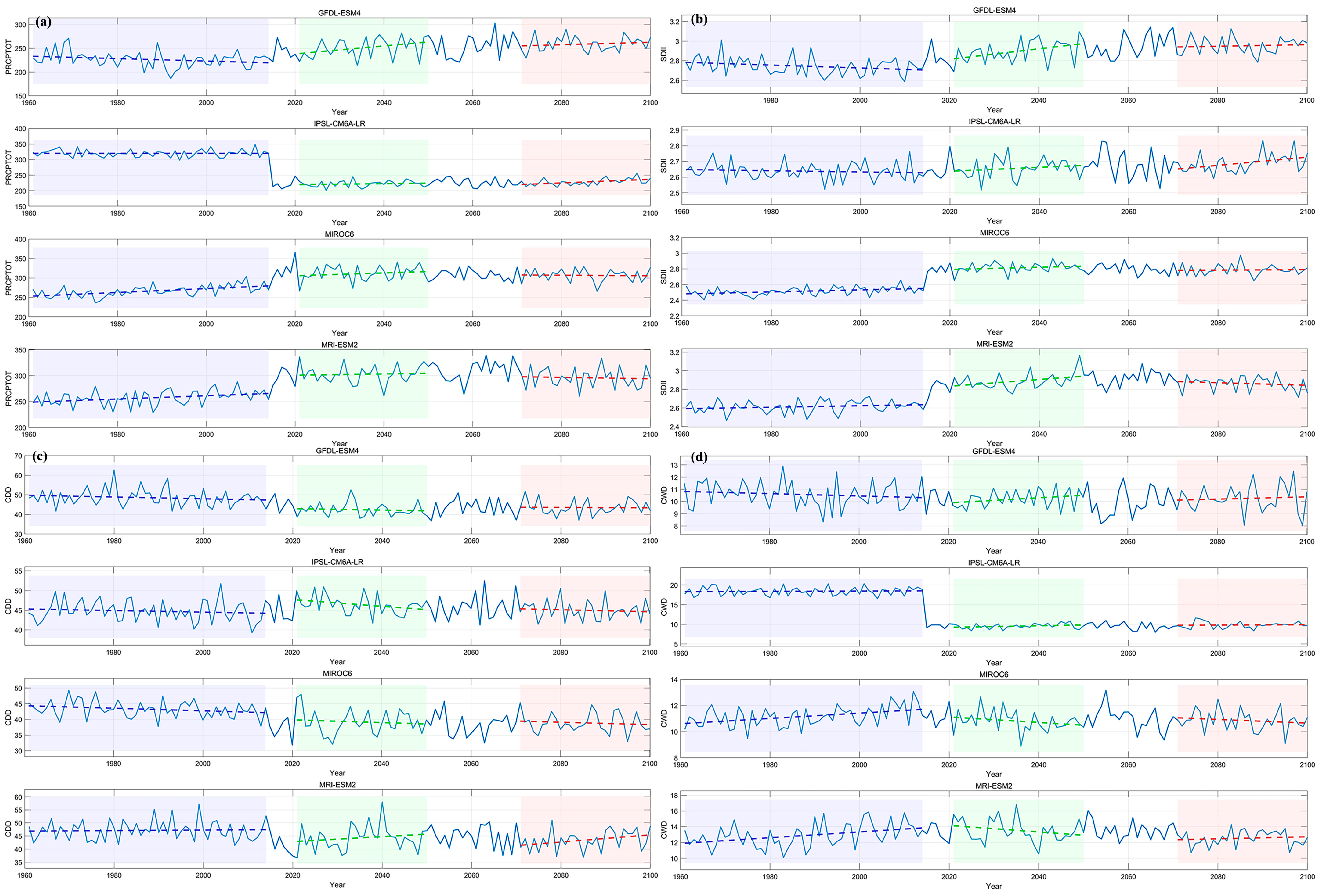
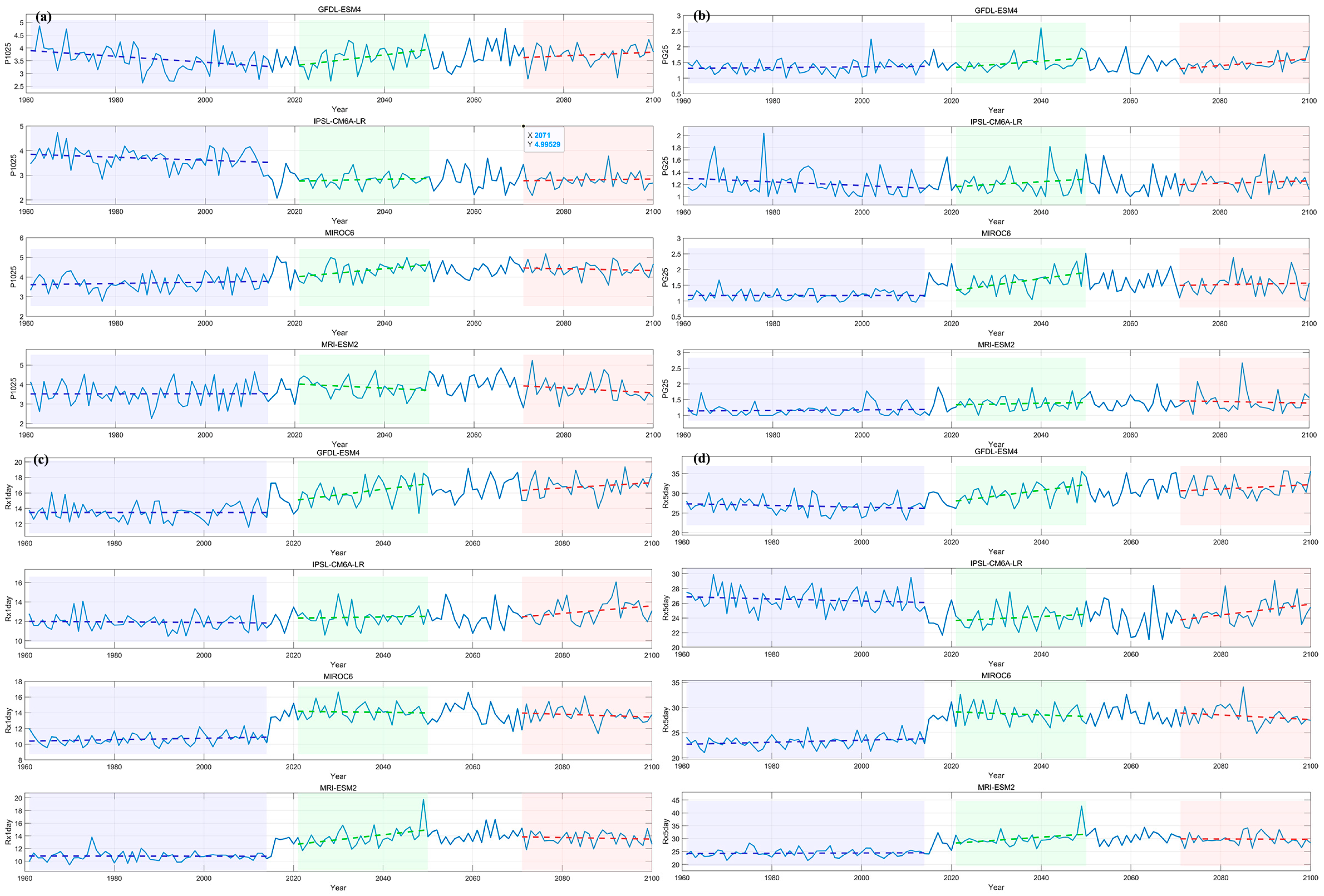
3.4. Analysis of Extreme Precipitation in the Future

Figure 6a–d and 6e–h depict the PRCPTOT annual average rates of change over the near future (NF: 2021–2050) and far future (FF: 2071–2100), respectively, relative to the observed data, while Figure 6i–p illustrate the corresponding SDII annual average percentage changes for both periods. The PRCPTOT change rates across the GCMs exhibited a spatially decreasing gradient from the central basin toward the southeastern and northwestern margins. For individual GCMs, the spatial distributions of PRCPTOT changes in the NF and FF were broadly consistent. Minimal variation in the PRCPTOT change rates was observed in the mountainous regions (Altai, Tianshan, Gangdise, Qilian, Helan, and Daxinganling Mountains) across both periods. In contrast, significant shifts occurred in the Gurbantunggut Desert, Taklimakan Desert, and Hami-Yinshan regions.

The GE and ME models displayed higher PRCPTOT change rates in the FF than in the NF within the central Taklimakan Desert, Gurbantunggut Desert, and Hami-Yinshan region (Figure 6a,b,e,f). Specifically, the PRCPTOT index in the Taklimakan Desert during the FF was six times the observed value, compared with a twofold increase in the NF. The MI and IL models (Figure 6c,d,g,h) showed similar spatial PRCPTOT patterns between the NF and FF, with substantial precipitation increases concentrated in the desert areas. For SDII changes in the GE and ME models (Figure 6i,j), the NF period featured reductions of approximately −10% in the peripheral mountain zones (Tianshan, Kunlun, Qilian, and Daxinganling Mountains), a +10% increase in the central desert, and a +30% increase in the Gangdise Mountains. By the FF (Figure 6m,n), SDII changes in the Tianshan, Kunlun, Qilian, and Taklimakan Desert areas declined relative to the NF, whereas the Gangdise Mountains experienced an increase. In the MI and IL models (Figure 6k,l), the NF SDII changes aligned with the other models but showed more pronounced negative values in select desert grids. During the FF (Figure 6o,p), SDII values in the central desert decreased markedly, with additional reductions observed in the southern and eastern regions, particularly in the Gangdise and Qilian Mountains.

Figure 7a–d,i–l display the annual average percentage changes in CDD (consecutive dry days) and CWD (consecutive wet days) indices for the four selected GCMs during the near future (NF: 2021–2050), while Figure 7e–h,m–p represent the corresponding annual average changes for the far future (FF: 2071–2100), both compared to observational baseline values. In the GE and ME models (Figure 7a,b,e–j), positive CDD changes were observed in select grids of the southeastern and northeastern regions (e.g., Qilian Mountains, Gangdise Mountains, and Daxinganling Mountains) across both periods. Conversely, most grids in the desert and northwestern/southwestern regions (e.g., Kunlun and Altai Mountains) exhibited negative changes. For the MI and IL models (Figure 7c,d,g,h), the CDD distributions in the NF aligned with those of the other models, but the FF projections revealed subtle shifts, particularly in the Altai and Tianshan Mountains, where some grids showed an >80% increase in CDD. Overall, the CDD changes for most grids ranged from −60% to +20% across all models and periods.

For the GE and ME models (Figure 7i,j), over 40% of the grids in the NF exhibited positive CWD changes, with negative values confined to scattered grids in the Tianshan, Kunlun, and Qilian Mountains. In the FF (Figure 7m,n), >80% of the grids showed positive CWD values, except in the Qinghai-Tibet Plateau spanning the Kunlun, Gangdise, Qilian, and Tianshan Mountains. In contrast, the MI and IL models (Figure 7k,l) displayed distinct CWD patterns in the NF, with >80% of the grids showing positive values and limited negative anomalies in the Tianshan, Kunlun, and Qilian Mountains. By the FF (Figure 7o,p), approximately half of the CWD changes became negative, concentrated in the mountainous (Altai, Tianshan, and Kunlun) and desert regions. Overall, CWD changes ranged from −10% to +100% across models and periods.

Figure 8a–d,i–l show the annual average percentage changes in P1025 (precipitation at the 25th percentile) and PG25 (precipitation intensity exceeding the 25th percentile) for the four selected GCMs during the near future (NF: 2021–2050), while Figure 8e–h,m–p illustrate the corresponding annual average changes for the far future (FF: 2071–2100). In the GE model (Figure 8a,e), most grids across the basin showed positive P1025 values during the NF, particularly in desert regions, while scattered negative values were observed in the Tianshan, Kunlun, and Qilian Mountains. The FF retained a spatially consistent pattern with the NF, although the magnitude of the positive values in the desert areas diminished. The ME model (Figure 8b,f) exhibited P1025 distributions similar to the GE model across both periods, but subtle differences emerged in the central desert and Gangdise Mountains during the NF period. For the MI and IL models (Figure 8c,d,g,h), P1025 changes ranged primarily between 0% and +10% in both NF and FF, with certain desert grids exceeding +20% changes. However, the grids in the Tianshan, Kunlun, and Gangdise Mountains consistently registered values around −5%.

In the GE and ME models (Figure 8i,j,m,n), PG25 changes in the Tianshan, Kunlun, Qilian, and Daxinganling Mountains were predominantly negative across periods, while grids in the Taklimakan Desert, Hami-Yinshan, and Gangdise Mountains showed increases of up to +40%. A notable decline in positive deviations occurred in the FF compared with the NF. The MI and IL models (Figure 8k,l,o,p) demonstrated that the PG25 changes were concentrated in the Taklimakan Desert, Gangdise Mountains of the Qinghai-Tibet Plateau, Hami-Yinshan, and Qilian Mountains. Unlike the GE and ME models, these models displayed significantly contrasting spatial patterns in the NF, with negative shifts dominating the mountainous regions (Altai, Tianshan, and Kunlun) and desert areas during the FF. Overall, the P1025 changes predominantly ranged from −5% to +20%, with higher variability in the desert regions. The PG25 values ranged from −40% to +40%, reflecting pronounced contrasts between precipitation extremes in arid basins and mountain zones.

Figure 9a–d,i–l show the annual average percentage changes in Rx1day (maximum 1-day precipitation) and Rx5day (maximum 5-day precipitation) for the four selected GCMs during the near future (NF: 2021–2050), while Figure 9e–h,m–p illustrate the corresponding far future FF 2071–2100) projections. Across most of the study region (IRB), the changes ranged from −30% to +100%. The GE and ME models (Figure 9a,b,e,f,i,j,m,n) exhibited nearly identical spatial patterns for both Rx1day and Rx5day across the NF and FF periods. Most grids showed positive values, with exceptions limited to scattered areas in the Altai Mountains, Tianshan Mountains, Kunlun Mountains, Qilian Mountains, and Hami region. In contrast, the MI and IL models (Figure 9c,d,g,h,k,l,o,p) displayed distinct spatial distributions compared to the GE and ME models, with generally lower-magnitude changes (predominantly < 20%) across most grids.

Figure 10 and Figure 11 show the temporal changes in each index and their corresponding trends. Figure 10a,b indicates that both PRCPTOT and SDII showed increasing trends in both the NF and FF periods. Figure 10c and d reveal decreasing trends in CDD and CWD, indicating more frequent alternation between precipitation and drought. Figure 11a,b demonstrates increasing trends in P1025 and PG25, suggesting an increase in the number of days with daily rainfall exceeding 10 mm and 25 mm. Figure 11c and d show that Rx1day and Rx5day also exhibit increasing trends. Overall, the IRB region experienced increased total precipitation, enhanced rainfall intensity, more frequent alternations between drought and precipitation, more frequent moderate-to-heavy rainfall days, and higher daily precipitation extremes in both the NF and FF periods.

4. Discussion

4.1. Model Performance and Uncertainties

The four CMIP6 GCMs evaluated in this study demonstrated a robust capability to replicate seasonal precipitation patterns, with the IL model showing the highest fidelity to observational data. While our projections broadly align with prior research indicating an intensifying humidification trend in Northwest China’s inland river basins [36], notable discrepancies emerged in magnitude. Specifically, our simulations under 1.5 °C warming yielded more conservative precipitation change estimates than those of the SSP126, SSP245, and SSP585 scenarios in existing studies. Consistent with regional climatology, elevated precipitation levels were identified in the Tianshan Mountains, Altai Mountains, and Qinghai-Tibet Plateau, a pattern corroborated by high-resolution modeling efforts [37]. Research suggests that uncertainties in hydrological projections primarily stem from three sources: internal variability, model uncertainty, and scenario uncertainty. In East Asia, model uncertainty dominates, followed by scenario uncertainty, with internal variability contributing the least [38]. As this study only involves the SSP1-1.9 scenario, the uncertainty in the simulation results is primarily attributed to model uncertainty. In topographically complex regions, the persistent uncertainty in precipitation simulation using GCMs is a key limiting factor. As noted by Prein et al. [39] and reinforced by recent CMIP6 evaluations, altitude-dependent biases in convective parameterization and snow-albedo feedback systematically skew precipitation simulations in mountainous and arid transition zones. For instance, CMIP6 models exhibit a 20.53 mm overestimation of orographic precipitation in the Kunlun Mountains when compared to ground-based radar observations [40].

4.2. Mechanisms Driving Hydrological Shifts

The reduction in CDD across the IRB—signaling more frequent and prolonged wet periods—is most pronounced in the Tianshan Mountains, Taklimakan Desert, and Kunlun-Gangdise ranges. These trends are likely driven by dual mechanisms: (1) Atmospheric Dynamics: Strengthened subtropical high-pressure systems over the Western Pacific and North America, amplified by Arctic amplification, enhance moisture transport into arid regions [41]. This mechanism aligns with the ‘warm Arctic–cold continent’ pattern, wherein reduced Arctic Sea ice intensifies meridional temperature gradients, reinforcing stationary Rossby waves that steer moisture-laden air masses into Northwest China. Concurrently, global warming has increased the Clausius-Clapeyron capacity of the atmosphere to hold moisture, thereby elevating precipitation efficiency in arid zones [42]. (2) Topographic Feedback: Warming-induced increases in atmospheric moisture enhance orographic precipitation on windward slopes (e.g., southeastern Kunlun Mountains). The declining snow cover and glacier mass in the Tianshan and Gangdise Mountains reduce the albedo, leading to earlier snowmelt and diminished cold-season precipitation recycling. Notably, the southeastern and northern Kunlun Mountains showed significant increases in consecutive wet days, while parts of the Gangdise Mountains on the Qinghai-Tibet Plateau displayed declining trends, reflecting localized microclimatic interactions.

4.3. Future Trends and Ecological Implications

Moderate rain days (>10 mm) are projected to increase basin-wide, while heavy rain days (>25 mm) will be concentrated in the mountains, deserts, and Gobi areas. However, the frequency of heavy rain may decline in far-future desert regions under aggressive climate mitigation. A rise in moderate-to-heavy rain over the Qinghai-Tibet Plateau’s arid zones could drive vegetation greening, as observed in recent satellite studies [43]. However, invasive species like Tamarix may exploit these conditions, threatening native ecosystems. The Rx1day and Rx5day precipitation peaks align with other indices, showing maxima in deserts, the Gangdise Mountains, and Yinshan-Daxinganling transition zones.

5. Conclusions

This paper evaluated the spatiotemporal evolution of extreme precipitation in the IRB under a new low radiative forcing scenario (SSP1-1.9) by employing four global climate models (GCMs: GFDL-ESM4, MRI-ESM2, MIROC6, and IPSL-CM6A-LR). Eight core extreme precipitation indices were analyzed to quantify changes during the near future (NF: 2021–2050) and far future (FF: 2071–2100) periods. The results showed that all four models were capable of capturing seasonal patterns and exhibited inherent uncertainty. The PRCPTOT in mountainous regions showed minimal variation, while desert areas were projected to experience a 2-6-fold increase in precipitation in the NF and FF. The SDII weakened by approximately −10% in mountainous areas but strengthened by around +10% in desert regions. Most mountainous areas showed an increase in CDD, whereas desert regions exhibited an extended CWD. Moderate rainfall (P1025) variations primarily ranged between −5% and +20%, with greater fluctuations observed in desert areas. Heavy rainfall (PG25) fluctuated between −40% and +40%, reflecting stark contrasts in extreme precipitation between arid basins and mountainous zones. Both Rx1day and Rx5day showed significant increases, which indicated heightened risks from extreme rainfall events in the future. Moreover, the IRB region experiences increased total precipitation, enhanced rainfall intensity, more frequent alternations between drought and precipitation, more frequent moderate-to-heavy rainfall days, and higher daily precipitation extremes in both NF and FF periods.

References

1. White, S.M.; Shelton, C.L.; Gelb, A.W.; Lawson, C.; McGain, F.; Muret, J.; Sherman, J.D. Principles of environmentally-sustainable anaesthesia: A global consensus statement from the World Federation of Societies of Anaesthesiologists. Anaesthesia 2022, 77, 201–212. [Google Scholar] [CrossRef] [PubMed]
2. De Nardi, S.; Carnevale, C.; Raccagni, S.; Sangiorgi, L. Climate Change Impact on Cereal Production in Northern Africa: A Comprehensive Modeling and Control Approach. IEEE Access 2025, 13, 5534–5550. [Google Scholar] [CrossRef]
3. Berg, P.; Moseley, C.; Haerter, J.O. Strong increase in convective precipitation in response to higher temperatures. Nat. Geosci. 2013, 6, 181–185. [Google Scholar] [CrossRef]
4. Donat, M.G.; Lowry, A.L.; Alexander, L.V.; O’Gorman, P.A.; Maher, N. More extreme precipitation in the world’s dry and wet regions. Nat. Clim. Change 2016, 6, 508–515. [Google Scholar] [CrossRef]
5. Zhang, W.X.; Zhou, T.J.; Wu, P.L. Anthropogenic amplification of precipitation variability over the past century. Science 2024, 385, 427–432. [Google Scholar] [CrossRef]
6. Wang, W.; Zhu, X.; Lu, P.; Zhao, Y.; Chen, Y.; Zhang, S. Spatio-temporal evolution of public opinion on urban flooding: Case study of the 7.20 Henan extreme flood event. Int. J. Disaster Risk Reduct. 2024, 100, 104175. [Google Scholar] [CrossRef]
7. Ding, T.; Xie, T.J.; Gao, H.; Zhang, S.Y. Alternation Between the Extreme Drought-Flood Event in the North China Plain in Summer 2024. Int. J. Climatol. 2025, 45, e8831. [Google Scholar] [CrossRef]
8. Zhang, W.X.; Zhou, T.J. Increasing impacts from extreme precipitation on population over China with global warming. Sci. Bull. 2020, 65, 243–252. [Google Scholar] [CrossRef]
9. Ben Alaya, M.A.; Zwiers, F.W.; Zhang, X. Probable maximum precipitation in a warming climate over North America in CanRCM4 and CRCM5. Clim. Change 2020, 158, 611–629. [Google Scholar] [CrossRef]
10. Pendergrass, A.G.; Coleman, D.B.; Deser, C.; Lehner, F.; Rosenbloom, N.; Simpson, I.R. Nonlinear Response of Extreme Precipitation to Warming in CESM1. Geophys. Res. Lett. 2019, 46, 10551–10560. [Google Scholar] [CrossRef]
11. Feng, T.C.; Zhu, X.; Dong, W.J. Historical assessment and future projection of extreme precipitation in CMIP6 models: Global and continental. Int. J. Climatol. 2023, 43, 4119–4135. [Google Scholar] [CrossRef]
12. Wu, R.G.; You, T.; Hu, K.M. What Formed the North-South Contrasting Pattern of Summer Rainfall Changes over Eastern China? Curr. Clim. Change Rep. 2019, 5, 47–62. [Google Scholar] [CrossRef]
13. Monerie, P.A.; Wilcox, L.J.; Turner, A.G. Effects of Anthropogenic Aerosol and Greenhouse Gas Emissions on Northern Hemisphere Monsoon Precipitation: Mechanisms and Uncertainty. J. Clim. 2022, 35, 2305–2326. [Google Scholar] [CrossRef]
14. Zhu, H.; Jiang, Z.; Li, L. Projection of climate extremes in China, an incremental exercise from CMIP5 to CMIP6. Science Bulletin 2021, 66, 2528–2537. [Google Scholar] [CrossRef] [PubMed]
15. Tian, Y.; Zhao, Y.; Li, J.; Xu, H.; Zhang, C.; Deng, L.; Wang, Y.; Peng, M. Improving CMIP6 Atmospheric River Precipitation Estimation by Cycle-Consistent Generative Adversarial Networks. J. Geophys. Res. Atmos. 2024, 129, e2023JD040698. [Google Scholar] [CrossRef]
16. Alexander, L.V.; Fowler, H.J.; Bador, M.; Behrangi, A.; Donat, M.G.; Dunn, R.; Funk, C.; Goldie, J.; Lewis, E.; Rogé, M.; et al. On the use of indices to study extreme precipitation on sub-daily and daily timescales. Environ. Res. Lett. 2019, 14, 125008. [Google Scholar] [CrossRef]
17. Bador, M.; Alexander, L.V.; Contractor, S.; Roca, R. Diverse estimates of annual maxima daily precipitation in 22 state-of-the-art quasi-global land observation datasets. Environ. Res. Lett. 2020, 15, 035005. [Google Scholar] [CrossRef]
18. Chen, C.-A.; Hsu, H.-H.; Liang, H.-C. Evaluation and comparison of CMIP6 and CMIP5 model performance in simulating the seasonal extreme precipitation in the Western North Pacific and East Asia. Weather. Clim. Extrem. 2021, 31, 100303. [Google Scholar] [CrossRef]
19. Xu, H.W.; Chen, H.P.; He, W.Y.; Chen, L.F. Contributions of Anthropogenic Greenhouse Gases and Aerosol Emissions to Changes in Summer Precipitation Over Southern China. J. Geophys. Res.-Atmos. 2024, 129, e2023JD040331. [Google Scholar] [CrossRef]
20. Han, T.T.; Guo, X.Y.; Zhou, B.T.; Hao, X. Recent Changes in Heavy Precipitation Events in Northern Central China and Associated Atmospheric Circulation. Asia-Pac. J. Atmos. Sci. 2021, 57, 301–310. [Google Scholar] [CrossRef]
21. Xue, S.Y.; Guo, X.H.; He, Y.H.; Cai, H.; Li, J.; Zhu, L.R.; Ye, C. Effects of future climate and land use changes on runoff in tropical regions of China. Sci. Rep. 2024, 14, 30922. [Google Scholar] [CrossRef] [PubMed]
22. Chen, L.Q.; Wang, G.J.; Miao, L.J.; Gnyawali, K.R.; Li, S.J.; Amankwah, S.O.Y.; Huang, J.; Lu, J.; Zhan, M. Future drought in CMIP6 projections and the socioeconomic impacts in China. Int. J. Climatol. 2021, 41, 4151–4170. [Google Scholar] [CrossRef]
23. Chen, X.G.; Li, Y.; Yao, N.; Liu, D.L.; Liu, Q.Z.; Song, X.Y.; Liu, F.; Pulatov, B.; Meng, Q.; Feng, P. Projected dry/wet regimes in China using SPEI under four SSP-RCPs based on statistically downscaled CMIP6 data. Int. J. Climatol. 2022, 42, 9357–9384. [Google Scholar] [CrossRef]
24. Xu, M.; Wang, P.S.; Zhang, X.; Ma, T.; Jin, J.L.; Kang, S.C.; Han, H.; Wu, H.; Hou, Z.; Li, X.; et al. Impacts of glacier shrinkage on peak melt runoff at the sub-basin scale of Northwest China. J. Hydrol. 2025, 654, 132953. [Google Scholar] [CrossRef]
25. Han, T.T.; Chen, H.P.; Hao, X.; Wang, H.J. Projected changes in temperature and precipitation extremes over the Silk Road Economic Belt regions by the Coupled Model Intercomparison Project Phase 5 multi-model ensembles. Int. J. Climatol. 2018, 38, 4077–4091. [Google Scholar] [CrossRef]
26. Chen, Z.W.; Zhang, X.F.; Chen, J.H. Monitoring Terrestrial Water Storage Changes with the Tongji-Grace2018 Model in the Nine Major River Basins of the Chinese Mainland. Remote Sens. 2021, 13, 1851. [Google Scholar] [CrossRef]
27. Guohua, F.; Heshuai, Q.; Xin, W.; Lei, Z. Analysis of spatiotemporal evolution of extreme monthly precipitation in the nine major basins of China in 21st century under climate change. J. Nat. Disasters 2016, 25, 15–25. (In Chinese) [Google Scholar]
28. Gupta, V.; Singh, V.; Jain, M.K. Assessment of precipitation extremes in India during the 21st century under SSP1-1.9 mitigation scenarios of CMIP6 GCMs. J. Hydrol. 2020, 590, 125422. [Google Scholar] [CrossRef]
29. Wu, J.; Gao, X.J. A gridded daily observation dataset over China region and comparison with the other datasets. Chin. J. Geophys. -Chin. Ed. 2013, 56, 1102–1111. [Google Scholar] [CrossRef]
30. Maraun, D. Bias Correction, Quantile Mapping, and Downscaling: Revisiting the Inflation Issue. J. Clim. 2013, 26, 2137–2143. [Google Scholar] [CrossRef]
31. Cannon, A.J. Multivariate quantile mapping bias correction: An N-dimensional probability density function transform for climate model simulations of multiple variables. Clim. Dyn. 2017, 50, 31–49. [Google Scholar] [CrossRef]
32. Maraun, D.; Widmann, M. Cross-validation of bias-corrected climate simulations is misleading. Hydrol. Earth Syst. Sci. 2018, 22, 4867–4873. [Google Scholar] [CrossRef]
33. Li, H.B.; Sheffield, J.; Wood, E.F. Bias correction of monthly precipitation and temperature fields from Intergovernmental Panel on Climate Change AR4 models using equidistant quantile matching. J. Geophys. Res.-Atmos. 2010, 115, 1–20. [Google Scholar] [CrossRef]
34. Ren, L.; Xue, L.Q.; Liu, Y.H.; Shi, J.; Han, Q.; Yi, P.F. Study on Variations in Climatic Variables and Their Influence on Runoff in the Manas River Basin, China. Water 2017, 9, 258. [Google Scholar] [CrossRef]
35. Wang, W.G.; Ding, Y.M.; Shao, Q.X.; Xu, J.Z.; Jiao, X.Y.; Luo, Y.F.; Yu, Z. Bayesian multi-model projection of irrigation requirement and water use efficiency in three typical rice plantation region of China based on CMIP5. Agric. For. Meteorol. 2017, 232, 89–105. [Google Scholar] [CrossRef]
36. Song, X.Y.; Xu, M.; Kang, S.C.; Wang, R.J.; Wu, H. Evaluation and projection of changes in temperature and precipitation over Northwest China based on CMIP6 models. Int. J. Climatol. 2024, 44, 5039–5056. [Google Scholar] [CrossRef]
37. Yuan, Y.Y.; Liao, B.Y. Evaluation of multi-source precipitation products for monitoring drought across China. Front. Environ. Sci. 2025, 13, 1524937. [Google Scholar] [CrossRef]
38. Wu, Y.; Miao, C.Y.; Slater, L.; Fan, X.W.; Chai, Y.F.; Sorooshian, S. Hydrological Projections under CMIP5 and CMIP6. Bull. Am. Meteorol. Soc. 2024, 105, E2374–E2389. [Google Scholar] [CrossRef]
39. Prein, A.F.; Rasmussen, R.; Castro, C.L.; Dai, A.G.; Minder, J. Special issue: Advances in convection-permitting climate modeling. Clim. Dyn. 2020, 55, 1–2. [Google Scholar] [CrossRef]
40. Fang, G.H.; Li, Z.; Chen, Y.N.; Liang, W.T.; Zhang, X.Q.; Zhang, Q.F. Projecting the Impact of Climate Change on Runoff in the Tarim River Simulated by the Soil and Water Assessment Tool Glacier Model. Remote Sens. 2023, 15, 3922. [Google Scholar] [CrossRef]
41. Xiao, D.; Ren, H.L. Interdecadal changes in synoptic transient eddy activity over the Northeast Pacific and their role in tropospheric Arctic amplification. Clim. Dyn. 2021, 57, 993–1008. [Google Scholar] [CrossRef]
42. Li, X.; Peachey, B.; Maeda, N. Global Warming and Anthropogenic Emissions of Water Vapor. Langmuir 2024, 40, 7701–7709. [Google Scholar] [CrossRef] [PubMed]
43. Liang, J.H.; Marino, A.; Ji, Y.J. Spatial and Temporal Change Characteristics and Climatic Drivers of Vegetation Productivity and Greenness during the 2001–2020 Growing Seasons on the Qinghai-Tibet Plateau. Land 2024, 13, 1230. [Google Scholar] [CrossRef]
Figure 1. Delineation of China’s Nine Major River Basins and Spatial Distribution of the Study Area. (a) Geographic location of the Nine Major River Basins in Chinas; (b) Inland River Basin of Northwest China.
Water 17 02009 g001
Figure 2. Seasonal changes of CN05.1 observation data and historical data of four GCMs in the IRB. (a) Observed precipitation in winter; (b) GE simulated winter precipitation; (c) ME simulated winter precipitation; (d) MI simulated winter precipitation; (e) IL simulated winter precipitation; (f) Observed precipitation in spring; (g) GE simulated spring precipitation; (h) ME simulated spring precipitation; (i) MI simulated spring precipitation; (j) IL simulated spring precipitation; (k) Observed precipitation in summer; (l) GE simulated summer precipitation; (m) ME simulated summer precipitation; (n) MI simulated summer precipitation; (o) IL simulated summer precipitation; (p) Observed precipitation in autumn; (q) GE simulated autumn precipitation; (r) ME simulated autumn precipitation; (s) MI simulated autumn precipitation; (t) IL simulated autumn precipitation.
Water 17 02009 g002
Figure 3. Changes in the bias percentage and the RMSE of the CMIP6 model for precipitation observations from 1961 to 2014. (a) Bias percentage of the GE model for precipitation observations; (b) Bias percentage of the ME model for precipitation observations; (c) Bias percentage of the MI model for precipitation observations; (d) Bias percentage of the IL model for precipitation observations; (e) RMSE of the GE model for precipitation observations; (f) RMSE of the ME model for precipitation observations; (g) RMSE of the MI model for precipitation observations; (h) RMSE of the IL model for precipitation observations.
Water 17 02009 g003
Figure 4. Bias percentage after correction for different CMIP6 GCMs from 1961 to 2014. (a) Bias percentage after GE model correction; (b) Bias percentage after ME model correction; (c) Bias percentage after MI model correction; (d) Bias percentage after IL model correction.
Water 17 02009 g004
Figure 5. Changes in the extreme precipitation indices observed by grids in the IRB from 1961 to 2014. (a) Annual average precipitation changes based on observational data; (b) Annual average PRCPTOT changes based on observational data; (c) Annual average SDII changes based on observational data; (d) Annual average CDD changes based on observational data; (e) Annual average CWD changes based on observational data; (f) Annual average P1025 changes based on observational data; (g) Annual average PG25 changes based on observational data; (h) Annual average Rx1day changes based on observational data; (i) Annual average Rx5day changes based on observational data.
Water 17 02009 g005
Figure 6. Calculate the PRCPTOT and the SDII annual average changes of all GCMs concerning the observed precipitation in the NF and the FF. (ad) represent the annual average change in PRCPTOT for GE simulations, ME simulations, MI simulations, and IL simulations versus observations in the NF, respectively; (eh) represent the annual average change in PRCPTOT for GE simulations, ME simulations, MI simulations, and IL simulations versus observations in the FF, respectively; (il) represent the annual average change in SDII for GE simulations, ME simulations, MI simulations, and IL simulations versus observations in the NF, respectively; (mp) represent the annual average change in SDII for GE simulations, ME simulations, MI simulations, and IL simulations versus observations in the FF, respectively.
Water 17 02009 g006
Figure 7. Calculate the annual average percentage change of CDD and CWD of all GCMs concerning the observed precipitation in the NF and the FF. (ad) represent the annual average change in CDD for GE simulations, ME simulations, MI simulations, and IL simulations versus observations in the NF, respectively; (eh) represent the annual average change in CDD for GE simulations, ME simulations, MI simulations, and IL simulations versus observations in the FF, respectively; (il) represent the annual average change in CWD for GE simulations, ME simulations, MI simulations, and IL simulations versus observations in the NF, respectively; (mp) represent the annual average change in CWD for GE simulations, ME simulations, MI simulations, and IL simulations versus observations in the FF, respectively.
Water 17 02009 g007
Figure 8. Calculate the annual average percentage change of P1025 and PG25 of all GCMs concerning the observed precipitation in the NF and the FF. (ad) represent the annual average change in P1025 for GE simulations, ME simulations, MI simulations, and IL simulations versus observations in the NF, respectively; (eh) represent the annual average change in P1025 for GE simulations, ME simulations, MI simulations, and IL simulations versus observations in the FF, respectively; (il) represent the annual average change in PG25 for GE simulations, ME simulations, MI simulations, and IL simulations versus observations in the NF, respectively; (mp) represent the annual average change in PG25 for GE simulations, ME simulations, MI simulations, and IL simulations versus observations in the FF, respectively.
Water 17 02009 g008
Figure 9. Calculate the annual average percentage change of Rx1day and Rx5day of all GCMs concerning the observed precipitation in the NF and the FF. (ad) represent the annual average change in Rx1day for GE simulations, ME simulations, MI simulations, and IL simulations versus observations in the NF, respectively; (eh) represent the annual average change in Rx1day for GE simulations, ME simulations, MI simulations, and IL simulations versus observations in the FF, respectively; (il) represent the annual average change in Rx5day for GE simulations, ME simulations, MI simulations, and IL simulations versus observations in the NF, respectively; (mp) represent the annual average change in Rx5day for GE simulations, ME simulations, MI simulations, and IL simulations versus observations in the FF, respectively.
Water 17 02009 g009
Figure 10. Historical, NF, and FF temporal changes and corresponding change trends in PRCPTOT, SDII, CDD, and CWD across the four models. Different colors in the graph represent different time periods and corresponding trends, with purple representing the historical period, green representing NF, and pink representing FF. (a) Historical, NF, and FF temporal changes and corresponding change trends in PRCPTOT across the four models; (b) Historical, NF, and FF temporal changes and corresponding change trends in SDII across the four models; (c) Historical, NF, and FF temporal changes and corresponding change trends in CDD across the four models; (d) Historical, NF, and FF temporal changes and corresponding change trends in CWD across the four models.
Water 17 02009 g010
Figure 11. Historical, NF, and FF temporal changes and corresponding change trends in P1025, PG25, Rx1day, and Rx5day across the four models. Different colors in the graph represent different time periods and corresponding trends, with purple representing the historical period, green representing NF, and pink representing FF. (a) Historical, NF, and FF temporal changes and corresponding change trends in P1025 across the four models; (b) Historical, NF, and FF temporal changes and corresponding change trends in PG25 across the four models; (c) Historical, NF, and FF temporal changes and corresponding change trends in Rx1day across the four models; (d) Historical, NF, and FF temporal changes and corresponding change trends in Rx5day across the four models.
Water 17 02009 g011