Article

Performance Study of a Sewage Collection Device for Seawater Pond Recirculating Aquaculture System

College of Marine Equipment and Mechanical Engineering, Jimei University, Xiamen 361000, China
*
Author to whom correspondence should be addressed.
Water 2025, 17(13), 1972; https://doi.org/10.3390/w17131972
Submission received: 3 June 2025 / Revised: 24 June 2025 / Accepted: 30 June 2025 / Published: 30 June 2025

Abstract

This study addresses the challenge of solid pollutant collection in seawater pond recirculating aquaculture by designing a novel funnel-shaped sewage collection device and evaluating its performance through Computational Fluid Dynamics (CFD) simulations and experimental validation. The results reveal that the device forms a rotating flow field, effectively concentrating solid particles in a central low-velocity zone with a diameter of approximately 2 m when the sewage pump is inactive. The optimal bottom dip angle for efficient sewage discharge is determined to be 21 degrees, with flow velocities near the outlet ranging between 0.031 and 0.062 m per second, sufficient to mobilize particles smaller than 5 mm. Prototype testing demonstrates a solid pollutant collection efficiency of 75.7 percent, confirming the device’s practical effectiveness in improving water quality and operational performance. This research offers a validated and efficient solution for solid waste management in aquaculture systems.

1. Introduction

With continuous improvements in living standards and increasing demand for aquatic products, there is growing attention on the quality and safety of aquatic products, especially aquaculture products. Water quality is a key factor that could impact the quality and safety of aquaculture products in the process of aquaculture production [1,2]. The traditional pond free-range farming mode inevitably encounters problems, such as the low utilization rate of aquaculture water resources and serious pollution. It is necessary to develop a new pond aquaculture mode due to the destruction of aquaculture ecology, frequent occurrence of aquaculture diseases, and increasing scarcity of aquaculture water resources [3,4,5,6]. To address these issues, intensive pond aquaculture has been identified as a significant development direction due to its obvious advantages of high yield, green advantage, and sustainable development [7,8].
The intensive pond aquaculture mode mainly consists of an aquaculture area and an ecological purification area. The aquaculture area accounts for about 2–5% of the pond area and it is used for raising fish at high density [9,10]. In the aquaculture area, the treatment of solid pollutants such as residual feed and feces generated during aquaculture is a key issue [11]. The solid pollutants that are not treated in time will give rise to increased levels of harmful substances such as ammonia nitrogen and nitrite, which can result in water quality deterioration and fish disease [12,13,14]. Thus, it is urgent to achieve timely and effective treatment of solid pollutants by developing a novel device.
In recent years, domestic and foreign scholars have conducted much research and exploration on the disposal of solid pollutants such as residual feed and feces. These studies are mainly related to recirculating aquaculture systems (RSA) and intensive pond aquaculture. The research methods can be divided into experiment, numerical simulation, and a combination of both. For the RSA, researchers mainly studied the influence of factors such as structural and operational parameters of the aquaculture tanks on their hydrodynamic characteristics and self-cleaning performance. These structural and operational parameters included the size of the fillet radius of the arc angle aquaculture tank, the position of the inlet pipe, the size of the inlet flow rate, the angle of the inlet jet, the flow rate of the bottom drainage, etc. [15,16,17]. Also, some researchers have studied the trajectory and residence times of different-sized particles in the tanks to explore the flushing effect of particles [18]. The research method of intensive pond aquaculture is similar to RSA. For instance, Stockton et al. [19] studied the effects of particle removal in mixed cell raceway and a Burrows pond rearing system with different structures. Sun and Liu [20] investigated the influence of the negative slope bottom of aquaculture tanks on the movement and transport capacity of particle pollutants in intensive pond aquaculture. Pfeiffer et al. [21] found that cyclone separators removed more than 90% of solid particulate matter with particle sizes greater than 250 μm in a tilapia factory recirculating water aquaculture system. However, the larger diameter of the particles it cleans up cannot comprehensively clean up the stains, and for pond recirculating aquaculture systems, the application is more limited, especially with regard to the collection devices (catchment areas), which are less studied.
Therefore, in this study, an innovative approach was adopted by combining the funnel-type collector with CFD simulation, investigate the flow characteristics and solid particle removal mechanism in the collector zone of a recirculating water aquaculture system in a seawater pond. Through the simulation of the internal flow field of the sewage collection device, the influence of the velocity distribution of the internal flow field on the deposition of solid particles and the effect of sewage discharge under different working conditions and different bottom dip angles are shown.

2. Materials and Methods

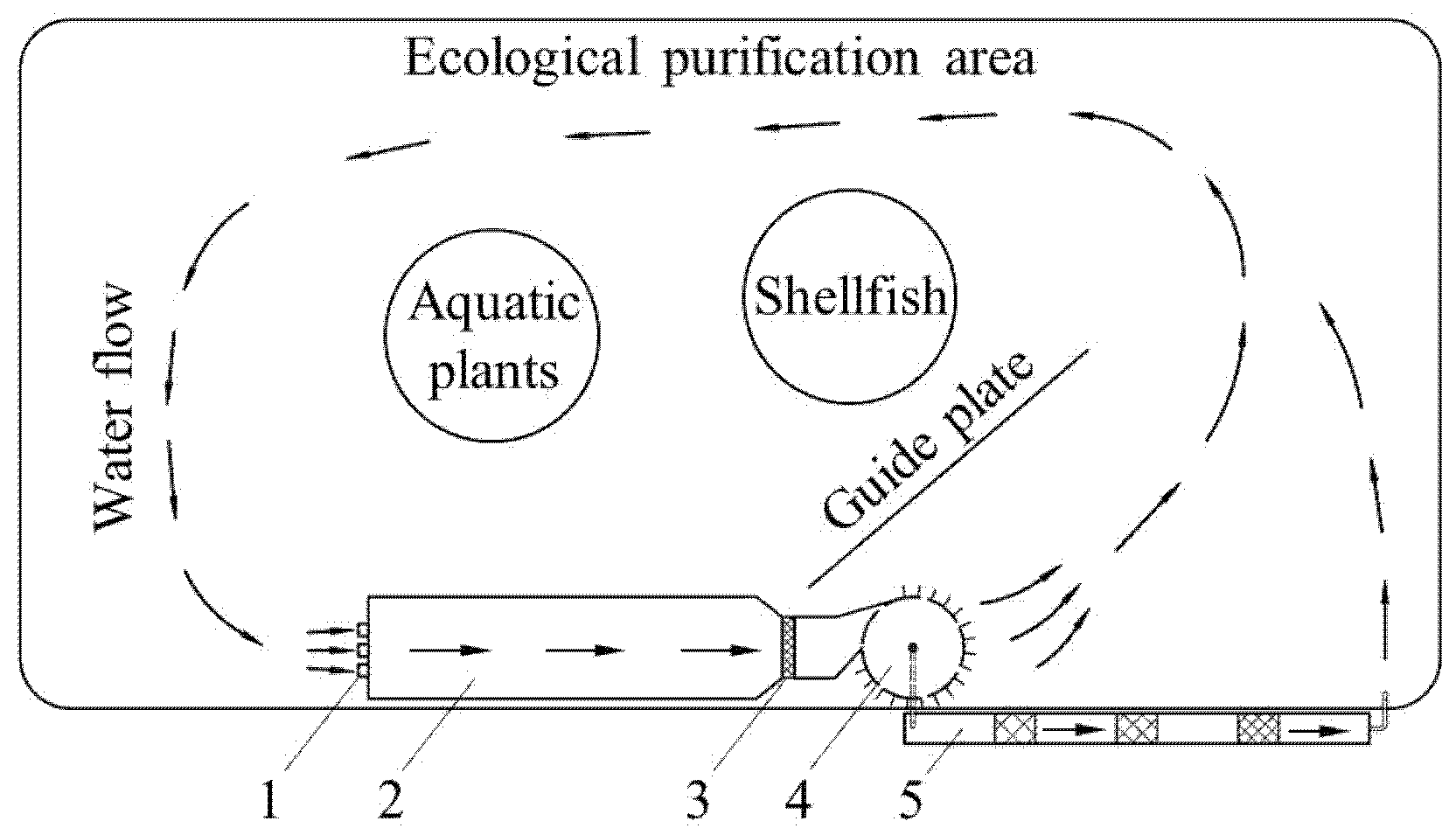
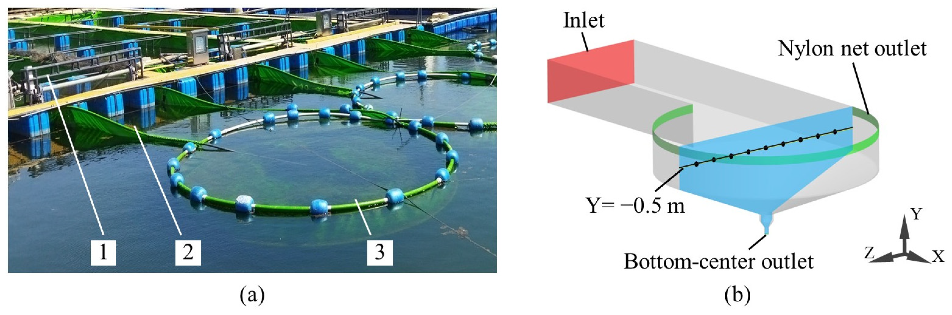
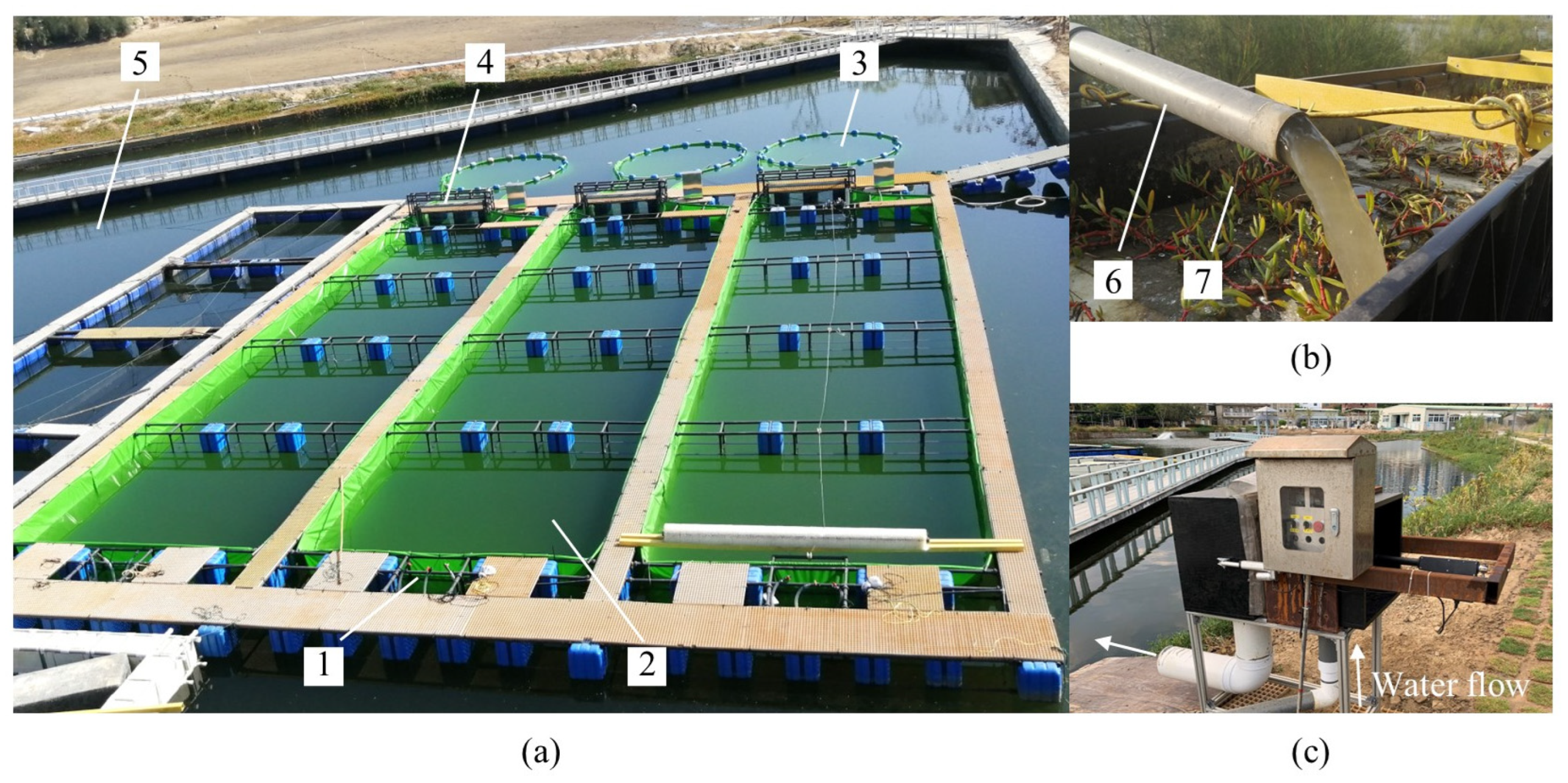
2.1. Description of the Seawater Pond Recirculating Aquaculture Mode

The seawater pond recirculating aquaculture mode divides the pond into an aquaculture area and an ecological purification area. The aquaculture area accounts for about 5% of the pond area, and the rest area is the ecological purification area. As shown in Figure 1, the water flow of the pond is recirculating. The aquaculture area mainly consisted of aeration plug-flow device, aquaculture tank, automatic barrier net replacement device, and sewage collection device. The aeration plug-flow device pours the water from the ecological purification area into the aquaculture tank. In the process of aquaculture, aeration plug-flow devices and a sewage collection device are used to ensure sufficient dissolved oxygen and favorable water quality in the aquaculture tank, further ensuring the safety and health of aquaculture production. The solid pollutants, such as residual feed and feces, flow into the sewage collection device for deposition under the action of water flow. The sewage pump regularly pumps the wastewater containing solid pollutants at the bottom of the sewage collection device to the filtering area on the bank. After multilayer filtration, the aquaculture tail water containing abundant nitrogen and phosphorus flows back to the ecological purification area. The part of the water is ecologically purified by shellfish and aquatic plants to achieve the principle of big ponds for water, small tanks for fish, and good water for good fish.

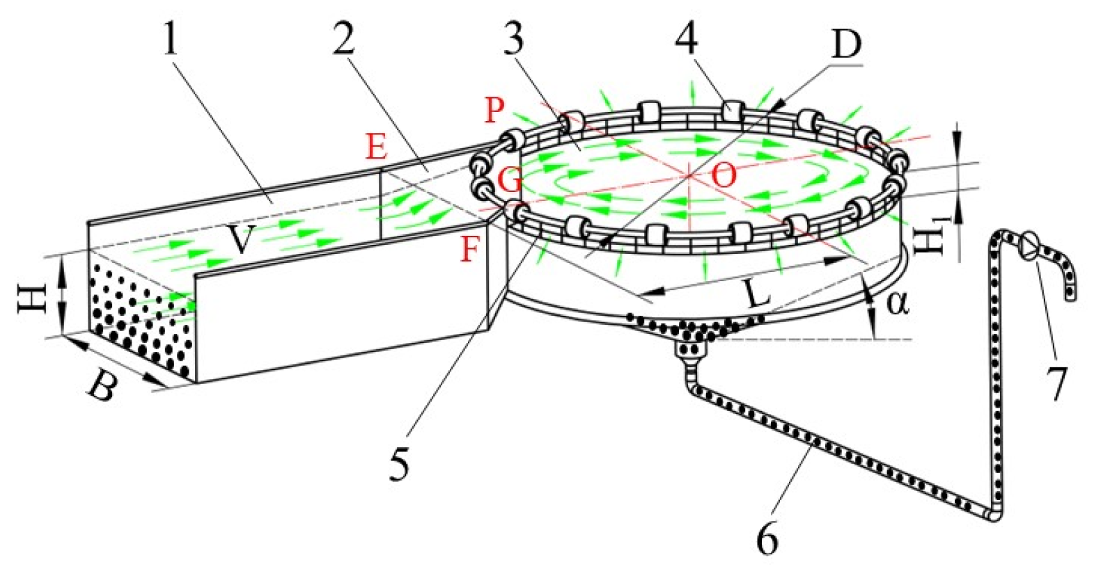
2.2. Structure of Sewage Collection Device

The sewage collection device mainly includes a water diversion trough, a sewage collecting cone trough and a sewage discharge module. As shown in Figure 2, the water diversion trough is divided into two parts: the constant section straight trough and the shrinkage trough. The width of the water inlet of the constant-section straight trough is B, and the water depth is H. The vertical distance from the front section of the shrinkage trough to the center O point of the sewage collecting cone trough is L. The long side EP of the shrinkage trough is tangent to the wall around the circle of the sewage collecting cone trough. The short side FG of the shrinkage trough intersects with the sewage collecting cone trough at point G in the quarter arc. The sewage collecting cone trough is made of tarpaulin, which is divided into a cylindrical section and a conical section. The diameter of the cylindrical section is D, and the depth is H. The bottom dip angle of the conical section is α, and its side unfolds as a sector. The α angle is ensured by controlling the radius and area of the sector. The sewage discharge module includes a sewage pipe and a sewage pump. The bottom-center outlet of the sewage collecting cone trough connects with the sewage pump through the sewage pipe with an inner diameter d. The floating balls are installed on an annular tube that could keep the sewage collecting cone trough on the water surface. A layer of nylon net with a height of H1 is connected underneath the annular tube. The water diversion trough guides the water flow into the sewage collecting cone trough along the tangential direction to form a vortex flow field. The vortex gathers the solid pollutants, and then these solid pollutants precipitate in the central area of the bottom. When the sewage pump is on-state, the water velocity increases in the area near the bottom-center outlet, and the bottom solid pollutants are pumped to the bank for filtration. In addition, part of the water can flow directly into the pond through the nylon net outlet for ecological purification during the operation process.

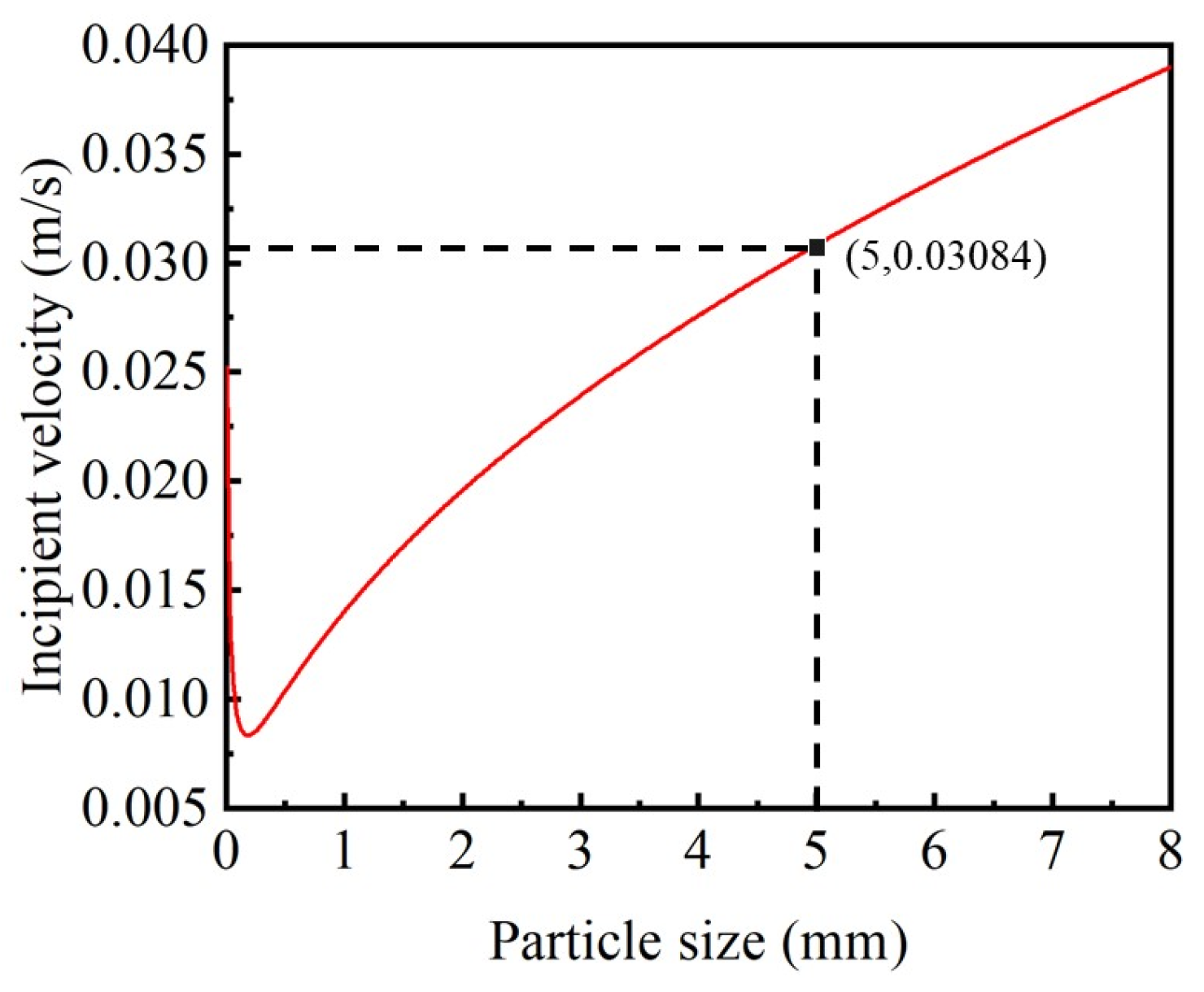
2.3. Force Analysis of Solid Particles in Water Flow

The solid particles in the flow can be divided into suspended particles and bedload particles according to the movement mode. The suspended particles are suspended in the water and move forward with the flow. The bedload particles sink at the bottom and slide or roll forward along the bottom. As suspended solid particles will be carried away by the water flow in time, this paper mainly analyzes the cleaning effect of bedload solid particles deposited at the bottom of the sewage collecting cone trough. The solid particles are simplified as spherical. The force on the solid particles on the inclined plane is shown in Figure 3, when the bottom particles start sliding in the water flow:
F D F s ( F P + F W + F G ) sin α
where FD is the drag force, Fs is the friction force, FG is the effective gravity underwater, FP is the adhesive force among particles, FW is the additional downforce caused by the water depth, and α is the bottom dip angle.
F s = f s ( F P + F W + F G ) cos α F L
where FL is the uplift force and fs is the coefficient of sliding friction, taken as 0.5.
The expressions of drag force FD, uplift force FL and effective gravity underwater FG of particles in water flow are as follows [22,23,24]:
F D = C D π 4 ρ 2 d s 2 v 0 2
where CD is the drag force coefficient, taken as 0.78, ρ is the water density, ds is the particle size, and v0 is the incipient velocity of the particle.
F L = C L π 4 ρ 2 d s 2 v 0 2
where CL is the uplift force coefficient, taken as 0.18.
F G = π 6 ( ρ s ρ ) g d s 3
where ρs is particle density and g is the gravitational acceleration.
In the study, Zhang [24] proposed the expressions for the adhesive force among particles FP and the additional downforce FW respectively:
F P = A P ρ d s ( γ γ c ) 6.6 ( ρ s ρ ρ ) g 0.33 υ 1.34
F W = A w ( γ γ c ) 6.6 π ρ d s g h δ
where AP is the adhesion coefficient and is taken as 3.45, γ′ is the dry bulk density of particles, γc′ is the stable dry bulk density of particles, γ′/γc′ = 0.85, υ is the kinematic viscosity of water, AW is the additional mass coefficient and is taken as 5.9 × 10⁻³, h is the water depth, and δ* is the film water thickness and is taken as 2.13 × 10⁻⁷ m.
From the above expression, it can be deduced that the required incipient velocity v0 for the sliding of solid particles is as follows:
v 0 8 ( f s cos α sin α ) 0.78 + 0.18 f s 0.5 × 1 6 ρ s ρ ρ g d s + 1.1 d s ( γ γ c ) 6.6 ( ρ s ρ ρ ) g 0.33 υ 1.34 + 0.0059 ( γ γ c ) 6.6 g h δ d s 0.5

2.4. Numerical Simulation

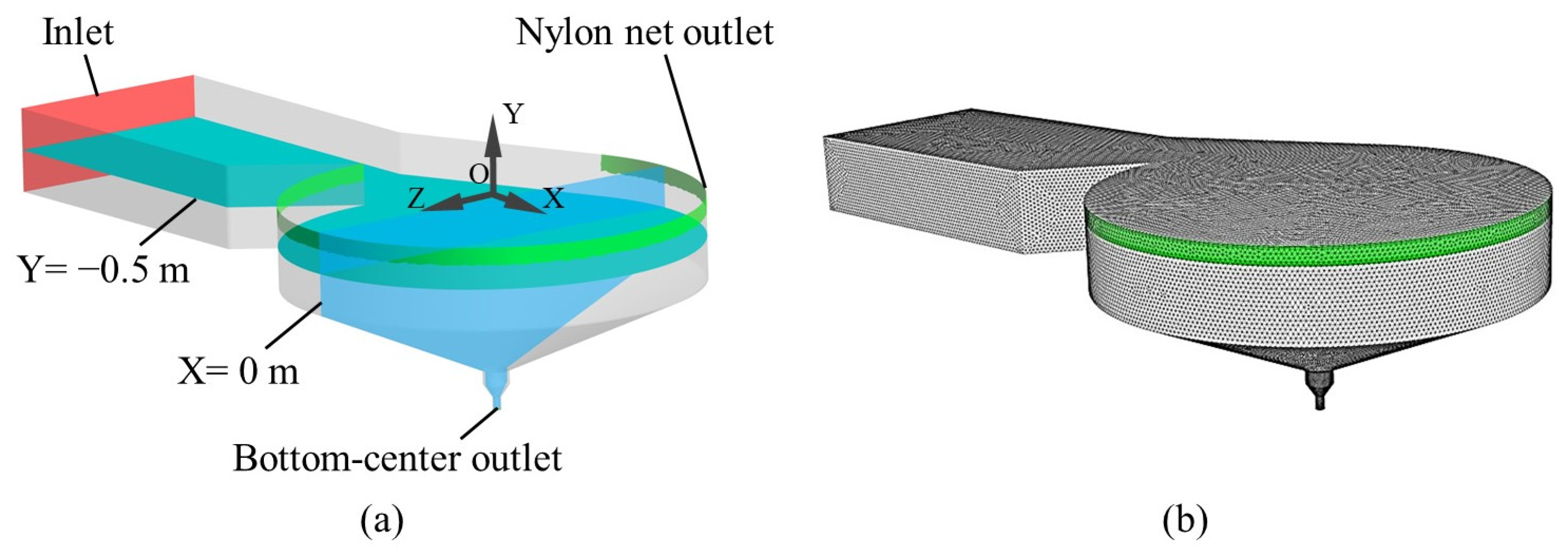
2.4.1. Meshing and Boundary Conditions

The computational fluid dynamics (CFD) software, Fluent 19.2, was utilised to simulate the internal flow field of the wastewater collection device. The Reynolds Stress Model (RSM) was selected as the turbulence model for this study due to its capacity to accurately capture the anisotropic turbulence and vortex flow characteristics inside the wastewater collection conical tanks relative to an isotropic eddy-viscosity model, which provides higher prediction accuracy for vortex-dominated flows in which turbulence anisotropy severely affects the particle deposition behaviour.
Considering the complexity of the structure of the sewage collection device, the geometry model of the fluid computational domain was appropriately simplified, as shown in Figure 4a. The main structure parameters of the fluid computational domain are consistent with the sewage collection device, as shown in Table 1. Fluent Meshing was used to divide the fluid computational domain into tetrahedral unstructured grids, and the bottom-center outlet was encrypted, as shown in Figure 4b.
The boundary condition of the inlet is set as velocity inlet, and the velocity is 0.033 m/s. The boundary condition of the outlet is set according to the working condition of the sewage collection device. The water flows only from the nylon net outlet when the sewage pump is off-state. The nylon net outlet is set as the pressure-outlet boundary. The water flows from both the nylon net outlet and the bottom-center outlet when the sewage pump is on-state. The nylon net outlet and the bottom-center outlet are set as pressure-outlet boundaries. The wall of the sewage collection device is set as a no-slip wall condition, and the water surface is set as the free surface boundary. The density of seawater is 1.03 × 10³ kg/m3, the dynamic viscosity of seawater is 1.05 × 10⁻³ Pa·s [25], and the gravitational acceleration is 9.81 m/s2.
To study the internal flow field velocity distribution of the sewage collection device, the two monitoring surfaces were set up. As shown in Figure 4a, the center point O on the surface of the sewage collecting cone trough is regarded as the coordinate origin. A longitudinal section at X = 0 m and a cross-section at Y = −0.5 m were selected as the monitoring surfaces.

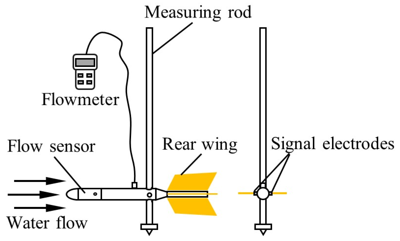
2.4.2. Experimental Measurements

The reliability of numerical models verified by experimental measurements is a significant method in the simulation research of the internal flow field of aquaculture tanks [26,27]. The water flow velocity was measured by the portable electromagnetic flowmeter (MGG-KL-DCB-I, Jiangsu Tongda Instrument Co., Ltd., Tangxia, China) in the present study. The measuring range of the flowmeter was within 0.005–10 m/s (the resolution is ±0.005) and the accuracy of ±1.0% of measured velocity. The electromagnetic flowmeter mainly includes a flow sensor, two signal electrodes, a rear wing, a measuring rod, and a flowmeter, as shown in Figure 5. The working principle of the electromagnetic flowmeter is based on the law of electromagnetic induction. The alternating magnetic field generates around the flow sensor when the flowmeter measures the water velocity. When water flows along the flow sensor, the induced potential is generated by cutting the magnetic field lines. The strength of the induced electromotive force is proportional to the magnitude of the flow velocity. After the induced electromotive force was collected by the signal electrode, it was converted to a flow velocity value by the flowmeter. The velocity of the water at different depths can be measured by adjusting the position of the flow sensor on the measuring rod.
The sewage collection device and experimental model are shown in Figure 6. The water diversion trough of the experimental model was a straight trough, without a shrinkage trough. The positions of the nine measurement points at a straight line on the plane X = 0 are as depicted in Figure 6b. The depth of points and the interval between adjacent points were 0.5 m. Each point was repeated three times, each measurement time was 60 s, and then the flow velocity values were averaged. These velocity values were used to validate the computational results. During the simulation, it was verified that the velocity of the inlet is 0.033 m/s, and the sewage pump is on-state.

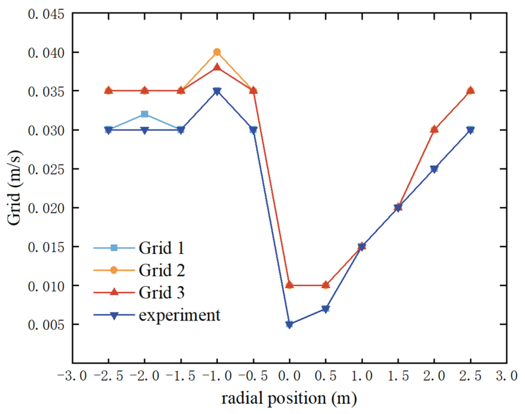
2.4.3. Model Verification

Before comparing the experimental data with the numerical simulation results, a grid independence analysis was conducted on the numerical simulation results of the three mesh groups. The corresponding grid numbers for Mesh 1, Mesh 2, and Mesh 3 were 0.78 million, 1.6 million, and 2.4 million, respectively. It was found that the results of Mesh 2 and Mesh 3 were essentially consistent, while Mesh 1 showed significant discrepancies, as illustrated in Figure 7. This indicates that the numerical simulation results are independent of the grid number when using Mesh 2 and Mesh 3. To save time and computational resources, Mesh 2 was adopted for the numerical simulation calculations. It shows that the experimental and the simulation results follow the same trend along the radial direction. It is noted that the standard deviation of the experimental results is larger near the center of the sewage collecting cone trough. There are three possible reasons: (1) as the experiment is carried out outdoors, the external environment has a certain influence on the measurement; (2) may be a vortex at the center of the sewage collecting cone trough leads flow instability, further influences flowmeter readings; (3) the water velocity is lowest near the center of the sewage collecting cone trough. When the water velocity was lower than the minimum value of the measuring range of the flowmeter, the reading of the flowmeter was 0 m/s.
The mean relative error between the experimental and the simulation results was used as the evaluation index for their consistency [18]. The expression for the relative error between experimental and simulation results is as follows:
δ = v s v e v e × 100 %
where vs is the flow velocity of the simulation, and ve is the flow velocity of the experiment. The average of all relative errors is the mean relative error, which is approximately 11%. It indicates that the simulation method is reasonable and accurate and can satisfy the study of the internal flow field of the sewage collection device.

3. Results and Discussion

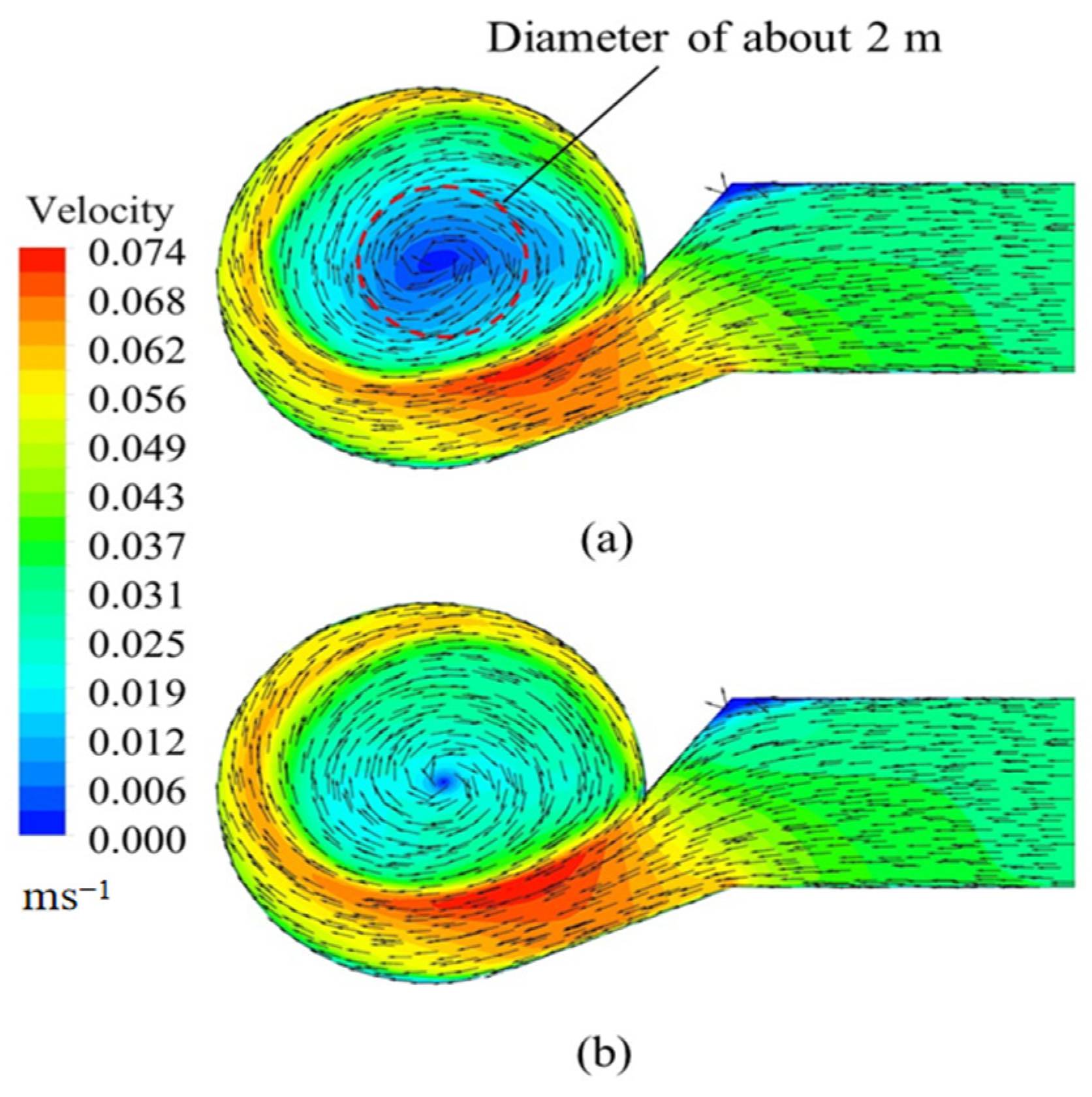
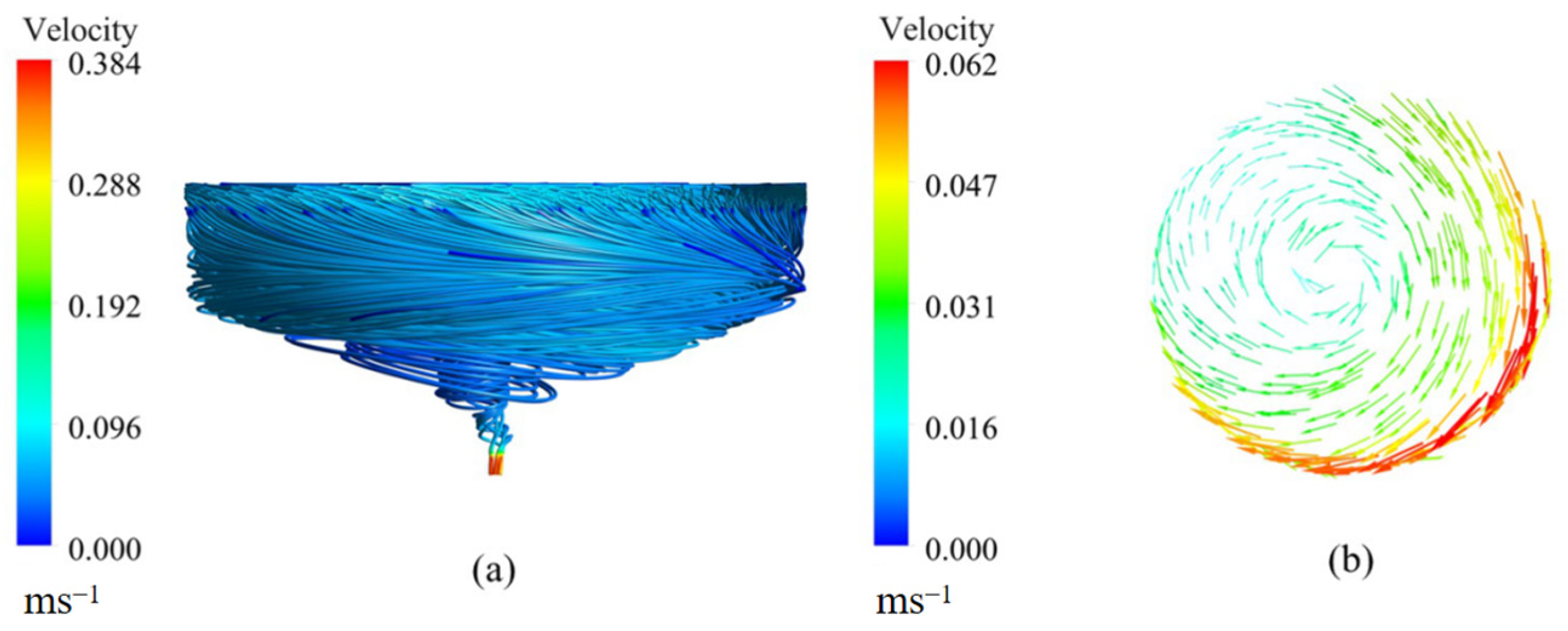
3.1. Distribution of Flow Field in Different States of the Sewage Collection Device

The distribution of the internal flow field of the sewage collection device under different working states is shown in Figure 8. Compared to the flow rate in Figure 7, the water velocity in Figure 8 is higher. The main reason is that the water diversion trough of the experimental model was a straight trough, without a shrinkage trough. Figure 8 shows that the water velocity increases through the shrinkage trough into the sewage collecting cone trough is accelerated. This indicates that the shrinkage trough is helpful to increase the water velocity in the sewage collecting cone trough, and it is conducive to the particles entering the cone trough with the water flow. The water flow forms a rotating flow field by the guidance of the side wall of the sewage collecting cone trough, as illustrated in Figure 8. Meanwhile, a low-velocity region was formed in the sewage collecting cone trough due to the gradual loss of partial energy of the water flow. The solid particles are mainly deposited at the bottom of this area. Figure 8a shows the flow field distribution at the monitoring surface of Y = −0.5 m as the sewage pump is off-state. It can be seen that the area of the low-velocity region is larger, mainly within a circular area of about 2 m in diameter. Figure 8b shows the flow field distribution at the monitoring surface of Y = −0.5 m as the sewage pump is on-state. Comparing Figure 8a,b, the area of the low-velocity region of the flow field is significantly reduced when the sewage pump is on-state. The flow velocity in the middle region is relatively higher and more uniformly distributed. It is conducive to promoting the solid particles to gather in the low-velocity region in the sewage collecting cone trough center with the water flow and finally discharged from the bottom-center outlet.

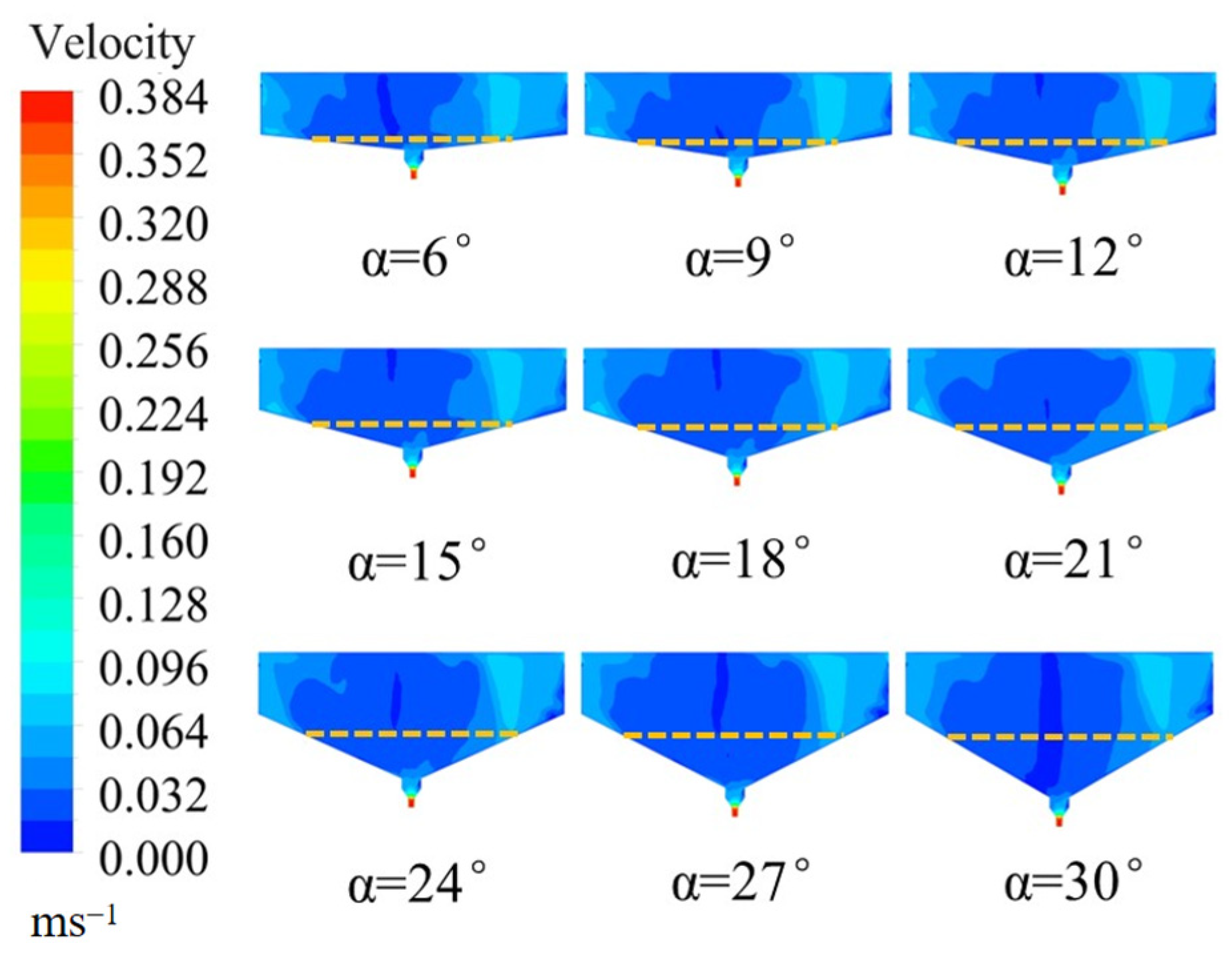
3.2. Influence of Different Bottom Dip Angles on Sewage Discharge Effect

To understand the influence of the bottom dip angle on the flow field inside the sewage collection device, Figure 9 shows the velocity distribution of the flow field at the monitoring surface of X = 0 m with nine different bottom dip angles α when the sewage pump is on-state. It can be seen that the area of the dark blue low-velocity region in the center of the sewage collecting cone trough gradually decreases as the bottom dip angle increases from 6° to 21°. Also, the velocity distribution is uniform. The flow velocity in the area near the bottom-center outlet is higher and the influence range is larger when the bottom dip angle is 21°. Then, the area of the dark blue low-velocity region gradually increases with the bottom dip angle increasing from 24° to 30°. In addition, the influence range of the higher flow velocity in the area near the bottom-center outlet begins to decrease.
The yellow dashed line shows the main lower flow velocity region near the bottom of the sewage collecting cone trough at different bottom dip angles, as shown in Figure 9. The discharge of the bottom particles can be achieved only if the lowest velocity of the water flow is bigger than the sliding incipient velocity of the particles. As shown in Figure 9, the distance from the left end of the yellow dashed line to the center of the sewage collecting cone trough is similar for different bottom dip angles. When the bottom dip angle is 21°, the length of the yellow dashed line is about 3.4 m, and the depth is about 1.3 m.
Figure 10a illustrates the particle separation performance of the sediment collection device with varying bottom inclination angles. The particle removal efficiency at the bottom outlet initially increased gradually before decreasing sharply with increasing inclination angle, reaching peak values at 21° and 24°. As evidenced in Figure 10b, the mean particle residence time at the bottom outlet remained stable when the inclination angle increased from 6° to 18°. However, further increasing the angle from 21° to 30° caused the residence time to first rise rapidly before declining, with the maximum value occurring at 27°. The upper outlet exhibited similar residence time trends versus inclination angle as the bottom outlet. This is because when the base inclination angle is less than 24°, as the angle increases from 6° to 18°, the volume variation in the conical section of the sediment-collecting hopper remains relatively small. Consequently, the flow field development inside the hopper exhibits similar patterns, leading to only minor differences in particle settling behavior. As a result, the increase in particle removal efficiency at the bottom outlet is gradual, and the average particle residence time shows little variation. However, as the base inclination angle further increases to 24°, the volume of the conical section expands significantly. This results in a longer flow field development time within the hopper, accompanied by a gradual reduction in flow velocity. These conditions enhance particle settling inside the hopper, thereby improving particle removal efficiency at the bottom outlet and increasing the average residence time of particles. When the base inclination angle exceeds 27°, the volume of the sediment-collecting hopper increases further, prolonging the particle residence time. However, under the influence of turbulent flow, a portion of downward-settling particles are re-entrained upward, thereby reducing the particle removal efficiency at the bottom outlet. At a base inclination angle of 30°, the particle removal efficiency at the bottom outlet is significantly lower than that at 27°, indicating fewer particles exiting through the bottom outlet. Consequently, the average particle residence time at the bottom outlet is shorter for the 30° configuration. In summary, for base inclination angles of 21° and 24°, the particle removal efficiency at the bottom outlet remains high (approximately 80%). However, at 24°, the average residence time is longer (~1000 s), whereas at 21°, it is comparatively shorter (~850 s). Considering both particle removal efficiency and average residence time, the sediment-collecting device demonstrates optimal performance at a base inclination angle of 21°.
When the bottom dip angle is 21°, the flow velocity near the bottom-center outlet is higher and the influence range is larger. It is more conducive to the aggregation and discharge of solid particles. Therefore, the flow field near the bottom of this sewage collecting cone trough needs to be further analyzed. Figure 11a shows the internal streamline diagram of the sewage collecting cone trough with the bottom dip angle of 21° when the sewage pump is on-state. It can be seen that the water flow near the bottom of the sewage collecting cone trough flows spirally to the bottom-center outlet. A circular cross-section with a diameter of 3.4 m was selected at a depth of 1.3 m (Y = −1.3 m) of the sewage collecting cone trough. The cross-sectional region is the range of the lower flow velocity area near the bottom of the sewage collecting cone trough. Figure 11b shows the velocity vector distribution on the cross-section. It can be seen that the velocity is lower in the central region of the cross-section and higher near the edges. Based on Equation (8), the dependency between the particle size and incipient velocity of the particle sliding when the density of solid particles is 1150 kg/m3 is shown in Figure 12. With the particle size increases, the incipient velocity decreases and then increases. In addition, the incipient velocity is less than 0.03084 m/s when the particle sizes are smaller than 5 mm. The solid particles deposited on the bottom surface are closer to the edge area. The velocity range of the edge area is mainly between 0.031 m/s to 0.062 m/s, which are all greater than 0.03084 m/s. It indicates that the flow velocity near the bottom surface can cause most of the solid particles to gather in the bottom-center outlet and discharge.

3.3. Prototyping Testing

The prototypes of the sewage collection device were regulated and installed at the end of the aquaculture tank based on the simulation results. The bottom dip angle was 21°. As shown in Figure 13a, the prototype aquaculture equipment configured in a 10-acre seawater pond has three aquaculture tanks (21 m × 5 m × 2 m). The aeration plug-flow device pushes oxygen-rich water into the aquaculture tank and exchanges the water about 18 times a day. Solid pollutants such as residual feed and feces flow into the sewage collection device under the action of the water and deposit. The sewage pump operates regularly four times a day (15 min/time) to discharge bottom solid pollutants into the bank filter tank. After several filters, the aquaculture tail water without solid particles eventually flows back into the ecological purification area to be purified. Thus, it can ensure that the water quality in the aquaculture tank is better and the pond has an ecological environment. During the fish culture trial, 2200 kg of grouper were reared in an aquaculture tank and fed 40 kg of feed a day. The solid pollutants generated in the aquaculture tank were estimated at 14 kg/day when assumed that solid pollutants produced 0.35 kg for every 1 kg of feed fish fed [28]. To know the application effect of the sewage collection device, the sewage pipe (Figure 13b) was connected to the sewage filtration equipment (Figure 13c). The sewage filtration equipment collected approximately 10.6 kg of solid pollutants. The collection ratio was about 75.7 %, and no obvious solid pollutants were precipitated at the bottom of the aquaculture tank. It indicates that the sewage collection device has a better operation effect.

4. Conclusions

Targeting the treatment of solid pollutants in the seawater pond recirculating aquaculture, this paper mainly explored the sewage collection-discharge performance of a novel sewage collection device. The effects of a device operation condition (on-off state of the sewage pump) and a key structural parameter (bottom dip angle of the sewage collecting cone trough) were considered in this study. The internal flow field characteristics of the sewage collection device were explored by the simulation method. In addition, the validity of the simulation method was confirmed by the experiment. Furthermore, a prototype of the sewage collection device was built based on the simulation results. Some conclusions can be drawn:
(1) When the sewage pump is off-state, a low-velocity region of about 2 m in diameter is formed in the sewage collecting cone trough, which is conducive to the deposition of the solid particles. When the sewage pump is on-state, the flow velocity in the sewage collecting cone trough increases, and the area of the low-flow velocity region is significantly reduced. It is helpful for promoting the solid particles deposited at the bottom of the low-velocity region to gather in the sewage collecting cone trough center and be removed.
(2) The flow velocity near the bottom-center outlet with the bottom dip angle of 21° is relatively high when the sewage pump is on-state. The flow velocity near the bottom surface is greater than the particle size of 5 mm solid particles sliding incipient velocity. It indicates that most of the solid particles deposited at the bottom of the sewage collecting cone trough could be removed.
(3) The results of the discharge test show that the operation effect of the sewage collection device is better. It shows that the CFD simulation results can provide guidance for the design of new and effective sewage collection devices.

Author Contributions

Conceptualization, Z.H.; Methodology, Z.C.; Validation, Y.Z.; Formal analysis, Y.Z.; Resources, Z.X.; Writing—original draft, Z.C. and Z.H.; Writing—review & editing, Z.X. All authors have read and agreed to the published version of the manuscript.

Funding

This research was funded by the Fujian Marine Economic Development Fund Project (FJHJF-L-2021-9) and the Natural Science Foundation of Fujian, China (Grant No. 2020J01693).

Data Availability Statement

The original contributions presented in this study are included in the article. Further inquiries can be directed to the corresponding author.

Acknowledgments

The authors gratefully acknowledge the support of the Fujian Marine Economic Development Fund Project (FJHJF-L-2021-9), Xiamen Municipal Bureau of Science and Technology(2024CXY0308) and the Natural Science Foundation of Fujian, China (Grant No. 2020J01693).

Conflicts of Interest

The authors declare no conflict of interest.

References

  1. You, G.; Xu, B.; Su, H.; Zhang, S.; Pan, J.; Hou, X.; Li, J.; Ding, R. Evaluation of Aquaculture Water Quality Based on Improved Fuzzy Comprehensive Evaluation Method. Water 2021, 13, 1019. [Google Scholar] [CrossRef]
  2. Zhang, X.; Zhang, Y.; Zhang, Q.; Liu, P.; Guo, R.; Jin, S.; Liu, J.; Chen, L.; Ma, Z.; Liu, Y. Evaluation and Analysis of Water Quality of Marine Aquaculture Area. Int. J. Environ. Res. Public Health 2020, 17, 1446. [Google Scholar] [CrossRef]
  3. Xiao, R.; Wei, Y.; An, D.; Li, D.; Ta, X.; Wu, Y.; Ren, Q. A review on the research status and development trend of equipment in water treatment processes of recirculating aquaculture systems. Rev. Aquac. 2018, 11, 863–895. [Google Scholar] [CrossRef]
  4. Han, P.; Lu, Q.; Fan, L.; Zhou, W. A Review on the Use of Microalgae for Sustainable Aquaculture. Appl. Sci. 2019, 9, 2377. [Google Scholar] [CrossRef]
  5. Jia, S.-P.; Wang, L.; Zhang, J.-M.; Zhang, L.; Ma, F.-R.; Huang, M.-L.; Liu, S.-S.; Gong, J.-H.; Zhang, M.; Yu, M.; et al. Comparative study on the morphological characteristics and nutritional quality of largemouth bass (Micropterus salmoides) cultured in an aquaculture system using land-based container with recycling water and a traditional pond system. Aquaculture 2022, 549, 737721. [Google Scholar] [CrossRef]
  6. Liu, X.; Shao, Z.; Cheng, G.; Lu, S.; Gu, Z.; Zhu, H.; Shen, H.; Wang, J.; Chen, X. Ecological engineering in pond aquaculture: A review from the whole-process perspective in China. Rev. Aquac. 2020, 13, 1060–1076. [Google Scholar] [CrossRef]
  7. Edwards, P. Aquaculture environment interactions: Past, present and likely future trends. Aquaculture 2015, 447, 2–14. [Google Scholar] [CrossRef]
  8. Boyd, C.E.; D’Abramo, L.R.; Glencross, B.D.; Huyben, D.C.; Juarez, L.M.; Lockwood, G.S.; McNevin, A.A.; Tacon, A.G.J.; Teletchea, F.; Tomasso, J.R., Jr.; et al. Achieving sustainable aquaculture: Historical and current perspectives and future needs and challenges. J. World Aquac. Soc. 2020, 51, 578–633. [Google Scholar] [CrossRef]
  9. Wang, Y.; Xu, G.; Nie, Z.; Li, Q.; Shao, N.; Xu, P. Effect of Stocking Density on Growth, Serum Biochemical Parameters, Digestive Enzymes Activity and Antioxidant Status of Largemouth Bass, Micropterus salmoides. Pak. J. Zool. 2019, 51, 1509–1517. [Google Scholar] [CrossRef]
  10. Hou, Y.; Li, B.; Xu, G.; Li, D.; Zhang, C.; Jia, R.; Li, Q.; Zhu, J. Dynamic and Assembly of Benthic Bacterial Community in an Industrial-Scale In-Pond Raceway Recirculating Culture System. Front. Microbiol. 2021, 12, 797817. [Google Scholar] [CrossRef]
  11. Becke, C.; Schumann, M.; Geist, J.; Brinker, A. Shape characteristics of suspended solids and implications in different salmonid aquaculture production systems. Aquaculture 2020, 516, 734631. [Google Scholar] [CrossRef]
  12. Huang, B.; Liu, B.; Lie, J.; Zhai, J.; Yan, K.; Liang, Y. The research on key technology and intelligent equipment of aquaculture welfare in industrial circulating water mode. J. Fish. China 2013, 37, 1750–1760. [Google Scholar] [CrossRef]
  13. Tom, A.P.; Jayakumar, J.S.; Biju, M.; Somarajan, J.; Ibrahim, M.A. Aquaculture wastewater treatment technologies and their sustainability: A review. Energy Nexus 2021, 4, 100022. [Google Scholar] [CrossRef]
  14. Bao, W.; Zhu, S.; Guo, S.; Wang, L.; Fang, H.; Ke, B.; Ye, Z. Assessment of Water Quality and Fish Production in an Intensive Pond Aquaculture System. Trans. ASABE 2018, 61, 1425–1433. [Google Scholar] [CrossRef]
  15. Davidson, J.; Summerfelt, S. Solids flushing, mixing, and water velocity profiles within large (10 and 150 m3) circular ‘Cornell-type’ dual-drain tanks. Aquac. Eng. 2004, 32, 245–271. [Google Scholar] [CrossRef]
  16. Zhang, J.; Jia, G.; Wang, M.; Cao, S.; Mkumbuzi, S.G. Hydrodynamics of recirculating aquaculture tanks with different spatial utilization. Aquac. Eng. 2022, 96, 102217. [Google Scholar] [CrossRef]
  17. Yu, L.; Xue, B.; Ren, X.; Liu, Y.; Xu, T.; Shi, X.; Hu, Y.; Zhang, Q. A study on the effect of single inlet pipe structure on the hydrodynamic characteristics of single-pass rectangular arc angle culture tanks. J. Dalian Ocean. Univ. 2020, 35, 134–140. [Google Scholar] [CrossRef]
  18. Liu, Y.; Liu, B.; Lei, J.; Guan, C.; Huang, B. Numerical simulation of the hydrodynamics within octagonal tanks in recirculating aquaculture systems. Chin. J. Oceanol. Limnol. 2016, 35, 912–920. [Google Scholar] [CrossRef]
  19. Stockton, K.A.; Moffitt, C.M.; Watten, B.J.; Vinci, B.J. Comparison of hydraulics and particle removal efficiencies in a mixed cell raceway and Burrows pond rearing system. Aquac. Eng. 2016, 74, 52–61. [Google Scholar] [CrossRef]
  20. Sun, D.; Liu, F. Pollution discharge performance and bottom slope optimization of aquaculture tanks for intensive pond aquaculture. J. Fish. China 2019, 43, 946–957. [Google Scholar]
  21. Pfeiffer, T.J.; Osborn, A.; Davis, M. Particle sieve analysis for determining solids removal efficiency of water treatment components in a recirculating aquaculture system. Aquac. Eng. 2008, 39, 24–29. [Google Scholar] [CrossRef]
  22. Chien, N.; Wan, Z.H. Mechanics of Sediment Transport; American Society of Civil Engineers: Reston, VA, USA, 2003. [Google Scholar]
  23. Li, L.L.; Zhang, G.G.; Wu, Z.; Gao, Y. Incipient motion velocity of non-cohesive uniform sediment particles on the positive and negative slopes. Sediment Res. 2016, 6, 54–59. [Google Scholar] [CrossRef]
  24. Zhang, H.W. A unified formula for incipient velocity of sediment. Hydraul. Eng. 2012, 43, 1387–1396. [Google Scholar] [CrossRef]
  25. Liu, S.G.; Liu, H.F.; Shu, H.S.; Zhao, D.; Xu, Z.; Zhang, L. Flow noise reduction of outboard valves based on internal flow path optimization. Harbin Eng. Univ. 2013, 34, 511–516. [Google Scholar] [CrossRef]
  26. Gorle, J.; Terjesen, B.; Summerfelt, S. Hydrodynamics of octagonal culture tanks with Cornell-type dual-drain system. Comput. Electron. Agric. 2018, 151, 354–364. [Google Scholar] [CrossRef]
  27. Xue, B.; Zhao, Y.; Bi, C.; Cheng, Y.; Ren, X.; Liu, Y. Investigation of flow field and pollutant particle distribution in the aquaculture tank for fish farming based on computational fluid dynamics. Comput. Electron. Agric. 2022, 200, 107243. [Google Scholar] [CrossRef]
  28. Ebeling, J.M.; Timmons, M.B. Recirculating Aquaculture Systems. In Aquaculture Production Systems; Cayuga Aqua Ventures, LLC: Freeville, NY, USA, 2012; pp. 245–277. [Google Scholar]
Figure 1. Schematic diagram of seawater pond recirculating aquaculture mode. 1: Aeration plug-flow device; 2: aquaculture tank; 3: automatic barrier net replacement device; 4: sewage collection device; 5: filtrating area.
Water 17 01972 g001
Figure 2. Structure of sewage collection device. 1: Constant section trough; 2: shrinkage trough; 3: sewage collecting cone trough; 4: floating ball and annular tube; 5: nylon net; 6: sewage pipe; 7: sewage pump.
Water 17 01972 g002
Figure 3. Particle force model.
Water 17 01972 g003
Figure 4. (a) Geometry model of the fluid computational domain. (b) Schematic diagram of grid division.
Water 17 01972 g004
Figure 5. Schematic diagram of the electromagnetic flowmeter.
Water 17 01972 g005
Figure 6. (a) Sewage collection device. (b) Position of the measurement points in the experimental model of the sewage collection device. 1: Automatic barrier net replacement device; 2: water diversion trough; 3: sewage collecting cone trough.
Water 17 01972 g006
Figure 7. Comparison between experiment and simulation.
Water 17 01972 g007
Figure 8. Distribution of the flow field in different states of the sewage collection device. (a) The sewage pump is off-state. (b) The sewage pump is on-state.
Water 17 01972 g008
Figure 9. Velocity distribution of the flow field at the monitoring surface of X = 0 mm with nine different bottom dip angles.
Water 17 01972 g009
Figure 10. Influence of bottom surface inclination on particle removal effect.cting cone trough with the bottom dip angle of 21°. (a) Particle removal rate; (b) Mean particle residence time.
Water 17 01972 g010
Figure 11. (a) Velocity streamlines of the sewage collecting cone trough with the bottom dip angle of 21°. (b) The velocity vector distribution on the cross-section.
Water 17 01972 g011
Figure 12. Dependency between the particle size and incipient velocity of the particle sliding.
Water 17 01972 g012
Figure 13. Prototype sewage discharge test. (a) Prototype of the aquaculture equipment. (b) Sewage discharge. (c) Sewage filtration equipment. 1: Aeration plug-flow device; 2: aquaculture tank; 3: sewage collection device; 4: automatic barrier net replacement device; 5: ecological purification area; 6: sewage pipe; 7: filter tank.
Water 17 01972 g013
Table 1. Main structure parameters of the fluid computational domain.
Structure ParameterSymbolValues
Width of the water inletB2.5 m
Depth of the water inletH1 m
The vertical distance from the front section of the shrinkage trough to the center O point of the sewage collecting cone troughL3.5 m
Diameter of the cylindrical section of the sewage collecting cone troughD5 m
Height of nylon net outletH10.2 m
Diameter of bottom-center outletd0.102 m
The bottom dip angle of the sewage collecting cone troughα6°, 9°, 12°, 15°, 18°, 21°, 24°, 27°, 30°
Disclaimer/Publisher’s Note: The statements, opinions and data contained in all publications are solely those of the individual author(s) and contributor(s) and not of MDPI and/or the editor(s). MDPI and/or the editor(s) disclaim responsibility for any injury to people or property resulting from any ideas, methods, instructions or products referred to in the content.

