Article

Assessing the Sensitivity of Sociotechnical Water Distribution Systems to Uncertainty in Consumer Behaviors: Social Distancing and Demand Changes During the COVID-19 Pandemic

1
Faculty of Civil and Environmental Engineering, Technion—Israel Institute of Technology, Haifa 32000, Israel
2
Department of Civil, Construction, and Environmental Engineering, North Carolina State University, 915 Partners Way, Raleigh, NC 27606, USA
*
Author to whom correspondence should be addressed.
These authors contributed equally to this work.
Water 2025, 17(13), 1965; https://doi.org/10.3390/w17131965
Submission received: 13 May 2025 / Revised: 25 June 2025 / Accepted: 27 June 2025 / Published: 30 June 2025
(This article belongs to the Section Water Resources Management, Policy and Governance)

Abstract

Water distribution systems (WDSs) exhibit intricate, nonlinear behaviors shaped by both internal dynamics and external influences. The incorporation of additional models, such as contamination or population models, further increases their complexity. This study investigated WDSs under various uncertainty scenarios to enhance system stability, robustness, and control. In particular, we built upon prior research by exploring an Agent-Based Modeling (ABM) framework integrated within a WDS, focusing on three types of uncertainties: (1) adjustments to existing probabilistic parameters, (2) variations in agent movement across network nodes, and (3) changes in agent distributions across different node types. We conducted our analysis using the virtual city of Micropolis as a testbed. Our findings indicate that while the system remains resilient to uncertainties in predefined probabilistic parameters, substantial and often nonlinear effects arise when uncertainties are introduced in agent mobility and distribution patterns. These results emphasize the significance of understanding how WDSs respond to external behavioral dynamics, which is essential for managing real-world challenges, such as pandemics or shifts in urban behavior. This study underscores the necessity for further research into broader uncertainty categories and emergent effects to enhance WDS modeling and inform decision-making.

1. Introduction

Water distribution systems (WDSs) are highly complex due to nonlinear hydraulics in looped pipelines. Beyond the mechanistic processes of water flows in pipe systems, actors and organizations interact with the water system and manipulate infrastructure components and adjust demands in response to system conditions. As a sociotechnical system, the interactions of consumers, decision-makers, operators, and WDS infrastructure lead to the emergence of hydraulic performance, including flows, pressures, and water quality in the network [1]. Recent advances in residential water-demand agent-based models provide a comprehensive overview of how consumer behavior has been represented in WDS simulations, highlighting both methodological approaches and data requirements [2].
One key condition to examine is the impact of different uncertainty scenarios [3]. The decisions and behaviors of consumers can propagate to affect the infrastructure components in unexpected ways. Uncertainty in behaviors can lead to disproportionate effects on demands, flows, and pressure in the WDS. For instance, pandemic-induced shifts in social-distancing policies have been coupled with hydraulic simulations to assess both contamination risk and altered demand profiles during COVID-19 [4].
Uncertainty in WDS models may also arise due to missing information, such as faulty sensor data, or from internal and external noise originating from various sources. Water utilities must adapt their operations in such cases, often without prior preparation for such uncertainties. Moreover, incorporating uncertainty into models is valuable for calibration [5], allowing for model parameters to be adjusted to align with real-world physical data. High-resolution smart-meter studies demonstrate how ten-minute-interval demand records can refine nodal demand patterns within EPANET frameworks, further underscoring the need to account for demand heterogeneity in sensitivity analyses [6].
It is important to distinguish between two related concepts [7,8,9]. Uncertainty analysis focuses on quantifying the extent of uncertainty in a given variable, whereas sensitivity analysis aims to identify the sources of uncertainty and assess how input uncertainties influence output variations. This research is focused on the sensitivity analysis of a sociotechnical WDS.
Numerous studies have analyzed WDS behavior under uncertain conditions. Ref. [10] highlighted the importance of such analyses for calibrating WDS models, representing real physical systems, and supporting decision-making. Since uncertainty in WDS parameters propagates to model predictions, understanding its effects is crucial. In this paper, we follow a similar approach but with key differences. Agent-Based Modeling (ABM) approaches have been developed to simulate the emergence of infrastructure performance and population behaviors that occur in sociotechnical WDSs. ABM was coupled with hydraulic simulation models to assess the effect of exposure and communication during contamination events [1,11], adoption of water reuse [12], and working from home during pandemics [13,14]. We used an ABM approach in this research, though we did not calibrate or compare ABM parameters with true values. Instead, we used an already near-realistic model, introducing uncertainties into ABM parameters rather than WDS parameters. We then assessed how these uncertainties affect selected model prediction parameters after simulating the ABM within a WDS. Similar to [10], we also analyzed the variance in model prediction uncertainty.
Ref. [15] explored methods to quantify and reduce uncertainty in WDS models for real-time control. The study examined uncertainties across multiple aspects: within the model itself, its parameters (e.g., pipe roughness), and measurement uncertainties in model inputs and outputs. While this aligns with [10], as both address uncertainties within the WDS model, our approach differs. We focused on an external model embedded within the WDS, analyzing its dynamic interactions with the system. Other studies have similarly examined uncertainties in WDS models. Refs. [16,17] discuss uncertainties within WDS models, with [16] distinguishing between two types: random (due to parameter variability) and fuzzy (due to incomplete information). Our study primarily deals with random uncertainty.
Unlike these studies, which focus on internal WDS uncertainties, we extend our investigation to a broader scope—examining the impact of external uncertainties on WDS behavior. This distinction is crucial, as external behavioral models, such as those related to COVID-19 responses or general urban movement patterns, can significantly influence WDS performance. For instance, during the spring 2020 COVID-19 lockdown, many utilities in North America and Europe reported residential water use increases of 20–30 percent during daytime hours, while commercial and industrial demand plunged by up to 40 percent [13,18]. Such abrupt demand shifts not only altered nodal pressure patterns but also drove unexpected changes in water age and quality, as lower turnover in certain mains led to chlorine decay and elevated microbial risk. By embedding social-behavioural models—capturing when and why people stayed home, shopped less, or adopted remote work—into hydraulic simulations, we can better anticipate these emergent pressure and quality excursions and inform adaptive operational strategies (e.g., targeted flushing or pressure adjustments).
Whereas previous research primarily addressed technical uncertainties, our study emphasizes social factors and their effects on system outcomes. Specifically, we analyze land-use patterns [19], COVID-19 transmission, and workforce movement across network nodes.
Uncertainty has also been explored within ABM studies, as seen in [20,21]. Several ABM studies across various disciplines have conducted uncertainty sensitivity analyses comparable to ours. Ref. [22], for example, assumed a probability distribution function (PDF) over 20 ABM parameters, using a uniform PDF to represent maximum uncertainty. This choice reflects a state of minimal knowledge about uncertainty, often measured through entropy. Their results indicated a negligible effect of uncertainty on selected performance variables—similar to our findings. However, ref. [23] adopted a different approach, assigning various PDFs suited to specific variables of interest. Their study introduced uncertainty into contamination event parameters within a WDS, focusing on physical infrastructure modeling. In contrast, our research introduces uncertainty into population dynamics and agent behaviors within the WDS network. Ref. [24] examined uncertainty within the social dimensions of ABM, distinguishing between input (epistemic) uncertainty, which pertains to uncertainties in model parameters, and model uncertainty, which involves uncertainties in agent interactions and assumptions. Our study primarily focuses on model uncertainty, assessing how external behavioral factors impact WDS dynamics.
Finally, by introducing several real-world-driven behavioral uncertainties into an ABM–WNTR coupling, we assess not only the robustness of standard probabilistic parameters (see the full description of the predefined probabilistic parameters in Section 3.4 and Section 3.4.1, and in Table A6) but also the sensitivity of the system to shifts in daily routines and land-use patterns. These insights are critical for utilities preparing for future disruptions—whether pandemics, major sporting events, or extreme weather—that fundamentally rewire how customers interact with the network.

2. Extension of Previous Research

This study extends the work of Vizanko et al. [14], which analyzed a modeling framework for simulating behavioral and demand changes during pandemics and assessing their impact on water quality in distribution systems. The framework utilizes Agent-Based Modeling (ABM) to represent individual behaviors and interactions, coupled with hydraulic simulations to evaluate water flow and quality. Additionally, it incorporates a susceptible–exposed–infected–recovered (SEIR) model for disease transmission and a Bayesian Belief Network (BBN) for predicting the adoption of preventive behaviors.
Building on this framework, our study examines system behavior under various uncertainty scenarios. Specifically, we explore uncertainties in (1) modulating existing probabilistic parameters, (2) agent movement across network nodes, and (3) changing the distribution of agents across different node categories. The primary objective of this study was to evaluate the ABM system’s response across different performance metrics under these uncertainty conditions. In particular, we aimed to identify conditions under which the system remains highly robust and conditions where it exhibits greater sensitivity. Our hypothesis suggested that the system should perform robustly under scenarios it was designed for, while unexpected scenarios may lead to variations in its response. To test this, we applied the following uncertainty methods:
  • Applying a uniform distribution to existing probabilistic parameters in the ABM system.
  • Introducing new variables that influence agents’ movement decisions within the network.
  • Modifying the distribution of agents among different node types.
Our key findings are as follows:
  • The system remains robust to uncertainty in existing probabilistic parameters, as expected, since it was designed for such variations.
  • The system exhibits different behaviors when agent movement is altered.
  • The system’s response becomes noticeably different—and even nonlinear—when agent distributions across node types are modified.
The latter two findings aligned with expectations, as the system was designed to respond differently under these conditions.
Finally, this paper is structured as follows:
  • Methods—Details the methodologies used in our analysis.
  • Case Study and Scenarios—Describes the various scenarios and conditions applied to assess uncertainty.
  • Results—Presents the findings from implementing different uncertainty methods.
  • Discussion and Conclusions—Summarizes key insights and implications of our results.

3. Methods

This section describes the ABM framework used for our simulations and outlines the different uncertainty methods applied to analyze how the ABM system responds to these uncertainties.

3.1. Overview

3.1.1. Purpose

The purpose of the ABM is to examine the effect of the adoption of COVID-19 prevention measures on demands and WDS performance. The ABM models the transmission of COVID-19, adoption of prevention measures, and water flows in a pipe network (Figure 1). The objective of this research is to evaluate the ABM simulation under various scenarios, particularly focusing on uncertainty conditions. Uncertainty is introduced in three ways: (1) modulating pre-existing probabilistic parameters, (2) altering agent movement dynamics, and (3) changing the distribution of agents across different node types (commercial, industrial, and residential).

3.1.2. Entities, State Variables, and Scales

The symbols used throughout this study, including work and home nodes, are listed in Table A5. Additionally, key decision variables such as working from home (WFH), dining out less, grocery shopping less, and personal protective equipment (PPE) usage are outlined in Table A6.
Agents represent individual water consumers, exerting demand at their respective nodes during each time step. Agents are mobile and travel among home, work, and leisure nodes. Each agent is characterized by multiple parameters, including COVID-19 transmission thresholds, and assigned home and work nodes and probabilities of interacting with television and radio (Table A5). Furthermore, agents have state variables that evolve throughout the simulation, encompassing COVID-19 status indicators, social distancing behavior decisions, and COVID-19 transmission timelines (Table A6). The COVID-19 status indicators include personal infection status, the infection status of friends and family, and exposure to COVID-19-related media.
The environment is defined by the hydraulic network, which determines the spatial distribution of nodes and classifies them as residential, commercial, or industrial. Residential nodes serve as home locations for agents, industrial nodes function as work locations, and commercial nodes are used for both work and leisure activities. Water-use patterns are specified in the hydraulic network file and vary according to node type.

3.1.3. Process Overview and Scheduling

The ABM process operates at multiple timescales: hourly, daily, and over the full simulation period. The following activities occur hourly (denoted as Ht in Appendix B): agent movement, COVID-19 transmission, water demand exertion, and interactions with mass media. Processes such as disease progression, adoption of preventive measures, and updates to demand patterns occur daily (denoted as Dt in Appendix B). Finally, the hydraulic simulation is executed at the conclusion of the 90-day simulation period (denoted as Step S1 in Appendix B).

3.2. Design Concepts

3.2.1. Theoretical and Empirical Background

COVID-19 Transmission: The transmission dynamics of COVID-19 in this framework are based on the SEIR model implemented in the ABM tool Covasim [5]. The mathematical relationships and parameter values defining the SEIR model were adopted from Covasim and integrated into our framework.
The SEIR model simulates disease spread based on agent interactions. When susceptible agents come into contact with infected agents, they have an age-dependent probability of becoming exposed. Once exposed, an agent transitions through different stages—pre-symptomatic or asymptomatic—also based on age-dependent probabilities. The duration spent in each stage follows a log-normal distribution, with distribution characteristics derived from multiple sources [5].
Asymptomatic agents progress directly to the recovered stage, where they remain for the rest of the simulation. Symptomatic agents, on the other hand, may experience disease progression through mild, severe, and critical stages, with each transition governed by age-dependent probabilities. Mild and severe cases recover after a designated period, while critical cases have a probability of progressing to a fatal outcome. Once recovered, agents no longer transmit or contract the disease.
A comparison of transmission dynamics between this framework and Covasim showed minimal discrepancies, validating the accuracy of our implementation.
Adoption of Prevention Measures: The adoption of prevention measures (PMs) is modeled using Bayesian Belief Networks (BBNs), which capture causal relationships between key variables. In this study, a Naïve Bayes classifier structure is employed to predict PM adoption based on factors such as an agent’s COVID-19 status, the status of their friends and family, and exposure to COVID-19-related media. Since these factors vary individually, the BBNs function as personalized decision-making models. Adoption decisions for each prevention measure are determined by the posterior probability generated by the BBN, which is continuously updated based on changes in the agent’s health status, social network conditions, and media exposure.
BBNs consist of a directed acyclic graph (DAG) defining variable relationships and conditional probability tables (CPTs) quantifying these relationships. By explicitly modeling dependencies and uncertainties, BBNs provide insights into how input variables influence adoption decisions. The BBN models utilize a Naïve Bayes classifier with forward selection to predict the adoption of specific PMs. Models for remote work and personal protective equipment (PPE) adoption incorporate Protection Motivation Theory (PMT) variables, while models predicting reduced grocery shopping and dining out rely on demographic and perception variables (Table A9) due to better performance metrics.
The DAGs of the four BBN decision-making models are illustrated in Figure A2, Figure A3, Figure A4 and Figure A5, while their performance metrics are detailed in Table A11.
Demand Changes: Demand changes are derived from empirical data published by Pesantez et al. [18], which includes hourly water demand records from approximately 20,000 smart meters covering both pre-pandemic and pandemic periods. Demand patterns were extracted from data collected during the first week of the pandemic (23–29 March 2020) and applied to all residential nodes. Compared to pre-pandemic patterns, morning and evening demand peaks shifted toward midday, leading to a flattened and overall reduced residential demand profile.

3.2.2. Individual Decision-Making

Agents make decisions to adopt social distancing behaviors based on their COVID-19 status and media exposure variables.

3.2.3. Interaction

Through the COVID-19 transmission model, infected agents expose susceptible agents at the node they currently occupy.

3.2.4. Heterogeneity

Agents are initialized with heterogeneous parameters and state variables, as detailed in Table A5 and Table A6. This heterogeneity influences COVID-19 transmission, agent interactions, social distancing behaviors, locations, and, subsequently, the variability in nodal water demand and water age.

3.2.5. Stochasticity

Even without the additional uncertainty analyses conducted in this study, the base ABM system incorporates stochasticity. Agent mobility is modeled stochastically, with agents randomly selected to move at each time step, while their destination nodes are predetermined during initialization. Several stochastic parameters are assigned to each agent at initialization (Table A6). Stochasticity is also embedded in COVID-19 contraction, progression through SEIR stages [5], and the probabilistic adoption of prevention measures based on BBN-generated posterior probabilities.

3.2.6. Observation

The number of agents in each stage of the COVID-19 transmission model (susceptible, exposed, infected, recovered, deceased) is monitored hourly. Additionally, water demand and water age are tracked for each node in the network. The adoption of prevention measures significantly alters disease transmission, resulting in changed water demands, modified flow patterns, and localized increases in water age.

3.3. Details

3.3.1. Implementation Details

Agents were implemented as classes using object-oriented programming in Python 3.8. These classes encapsulate both the attributes and methods defining each agent’s state and behavior. Hydraulic simulation was conducted using the Water Network Tool for Resiliency (WNTR), which is built upon EPANET version 2.2 [25,26].

3.3.2. Initialization

COVID-19 infection thresholds are initialized using a log-normal distribution (Table A5), and 0.1% of the population is initially set as exposed ( S = exposed ). Each agent is randomly assigned a home node and a work node.

3.3.3. Input Data

The model requires several input datasets, including the following:
  • COVID-19 transition values.
  • Risk perception variables for Bayesian Belief Network (BBN) training.
  • Hydraulic network data, including pipes, pumps, tanks, valves, and demand patterns.

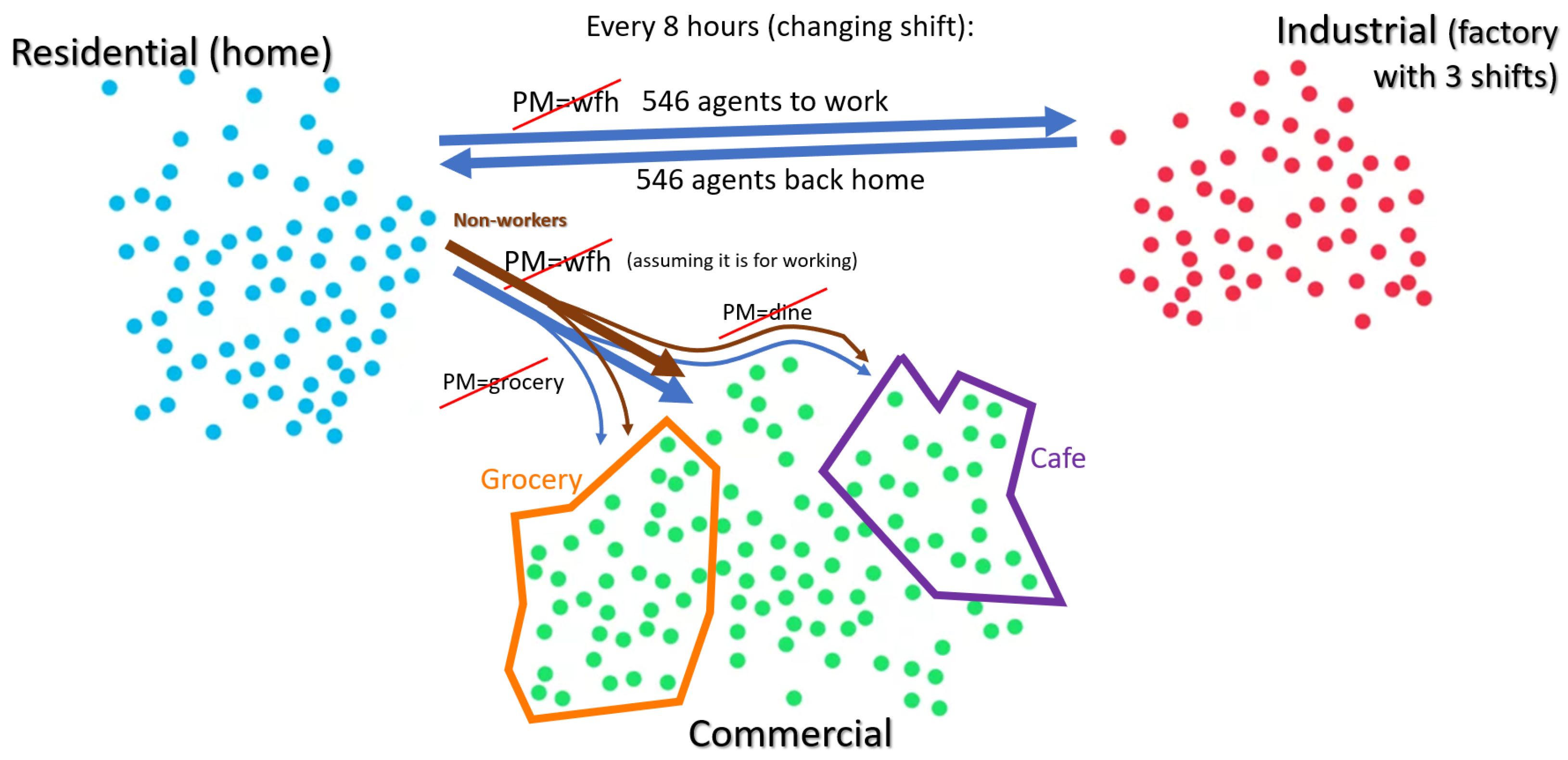
3.3.4. Movement Submodel

Agent movement follows two primary bi-directional pathways between node types (Figure 2):
  • Residential to Commercial Movement: Agents move between residential and commercial nodes based on their prevention measure (PM) adoption:
    Agents not adopting the dine-out PM move to café nodes (subset of commercial nodes).
    Agents not adopting the grocery PM move to grocery nodes (subset of commercial nodes).
    Agents not adopting the work-from-home (WFH) PM move to any commercial node.
    Movement from commercial to residential nodes (i.e., returning home) has no restrictions.
  • Residential to Industrial Movement: Initially, a predefined number of agents (e.g., 1092) are placed at industrial nodes. Every 8 h, half of these agents ( 1092 / 2 ) are replaced with agents from residential nodes at specific time steps: 1:00, 9:00, and 17:00.
    Only agents that do not adopt the WFH PM move to industrial nodes. Movement from industrial to residential nodes (returning home) has no restrictions.

3.4. Uncertainty Submodel

The ABM framework incorporates multiple uncertainty factors to evaluate their impact on system behavior. These modifications include the following:
  • Number of Daily Contacts: Uncertainty is introduced in the number of agents potentially exposed to infectious agents during movement between nodes.
  • Exposure Rate: The probability of exposure for selected agents is modeled with uncertainty.
  • Media Exposure: The probability of agents consuming COVID-19-related information via television or radio is subject to uncertainty.
  • Uncertainty in BBN Output: The BBN output determining PM adoption is probabilistic rather than deterministic. Agents update their status based on this probability, introducing uncertainty.
  • Exposed Agents’ Condition: Uncertainty is incorporated into the process of determining the health condition of newly exposed agents.
  • Worker Mobility: While movement between node types follows specific rules, exceptions allow agents to move from residential to commercial nodes for non-work-related purposes, with a probabilistic constraint.
  • Node Type Distribution: The initial distribution of agents across industrial, café, commercial, and residential nodes is subject to uncertainty.

3.4.1. Uncertainty in COVID-19 Transmission Model

This section describes how uncertainty was introduced into the COVID-19 transmission model.
The threshold value governing transmission probability is sampled from a predefined range. For example, a threshold of 0.5 may vary within [0.4, 0.6] or [0.3, 0.7]. Alternatively, noise can be added using an adjustable function, such as r a n < 0.5 + 0.2 · n o i s e , where parameters (0.5, 0.2) define the base probability and scaling factor, and n o i s e follows a mean-zero distribution.
Table A6 lists all state variables in the ABM, highlighting key parameters (probabilistic parameters) modified in the COVID-19 transmission model:
  • Exposure rate ( e r ).
  • Non-residential exposure rate ( e n r ).
  • Probability of listening to the radio ( P R ).
  • Probability of watching TV ( P T V ).
The primary objective was to evaluate the robustness of the ABM system under uncertainty. We focused on existing areas in the model where some level of fixed uncertainty already existed. Specifically, we examined cases where a variable is assigned an initial value, a uniformly distributed random number r a n U ( 0 , 1 ) is generated, and the variable is updated if r a n falls below a predefined threshold. Otherwise, the initial value remains unchanged.

3.4.2. Worker Mobility

Agent movement rules were previously outlined in Figure 2. Initially, only workers traveled between residential and commercial nodes. To account for non-work-related movement, a new probability variable was introduced, allowing agents to move from residential to commercial nodes with some probability.

3.4.3. Node Type Distribution

The original ABM code assumed a fixed distribution of agents across node types (industrial, café, commercial, and residential). To incorporate uncertainty, we introduced stochastic variation in agent distribution among these node types. This modification aligns with the broader objective of testing how uncertainty influences system behavior. Rather than introducing uncertainty indiscriminately, we targeted areas where it could significantly affect outcomes. The variability in node distribution represents different city structures—for example, industrial-heavy, residential-heavy, or commercially dominant urban environments. To ensure fair comparisons across simulations, the total number of agents in the system remains constant while their distribution across node types varies stochastically.

3.4.4. Statistical Significance

In our sensitivity experiments, each uncertainty scenario was run using the same set of pre-assigned random seeds and noise streams as the base (no-uncertainty) model. By preserving the exact stochastic realizations across paired simulations, we ensured that any observed differences in output—whether in SEIR peaks, water age, or demand patterns—arose solely from the modification of model structure or parameter values, rather than from sampling variability. This “organized seeds” approach is a common practice in agent-based sensitivity studies (e.g., [20,22]) and obviates the need for large-sample hypothesis testing: if the mean difference between two paired runs exceeds the natural run-to-run variation under identical seeds, it reflects a structural sensitivity rather than random noise. For smaller effects—where paired differences remain within the inherent stochastic envelope—we acknowledge that these perturbations are indistinguishable from background variability, reinforcing our conclusion that the system is robust to such parameter changes.

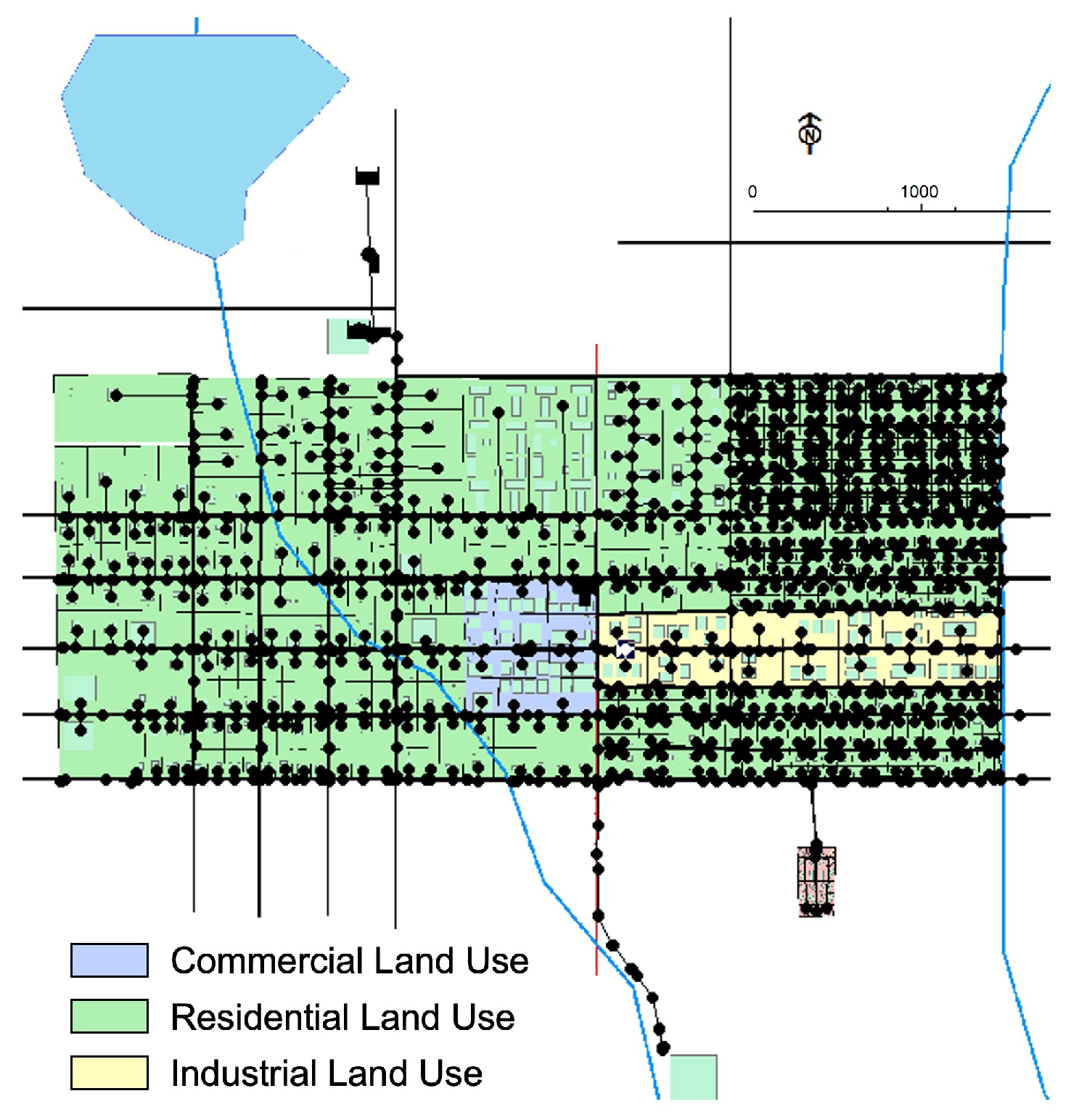
4. Case Study and Scenarios

For our simulations, we utilized the Micropolis [27] virtual city (Figure 3). The Micropolis water system consists of 458 terminal nodes, representing a population of approximately 4600 residents. These nodes include
  • 434 residential connections,
  • 15 industrial connections,
  • 9 commercial connections.
The total daily water demand is 4.54 ML/day, with distinct diurnal patterns assigned to each node type.
To facilitate scenario comparisons, we used organized simulation seeds corresponding to specific simulation indices. In the following, Table 1 presents the summary of all generated modifications in the ABM model to include uncertainties.

5. Results

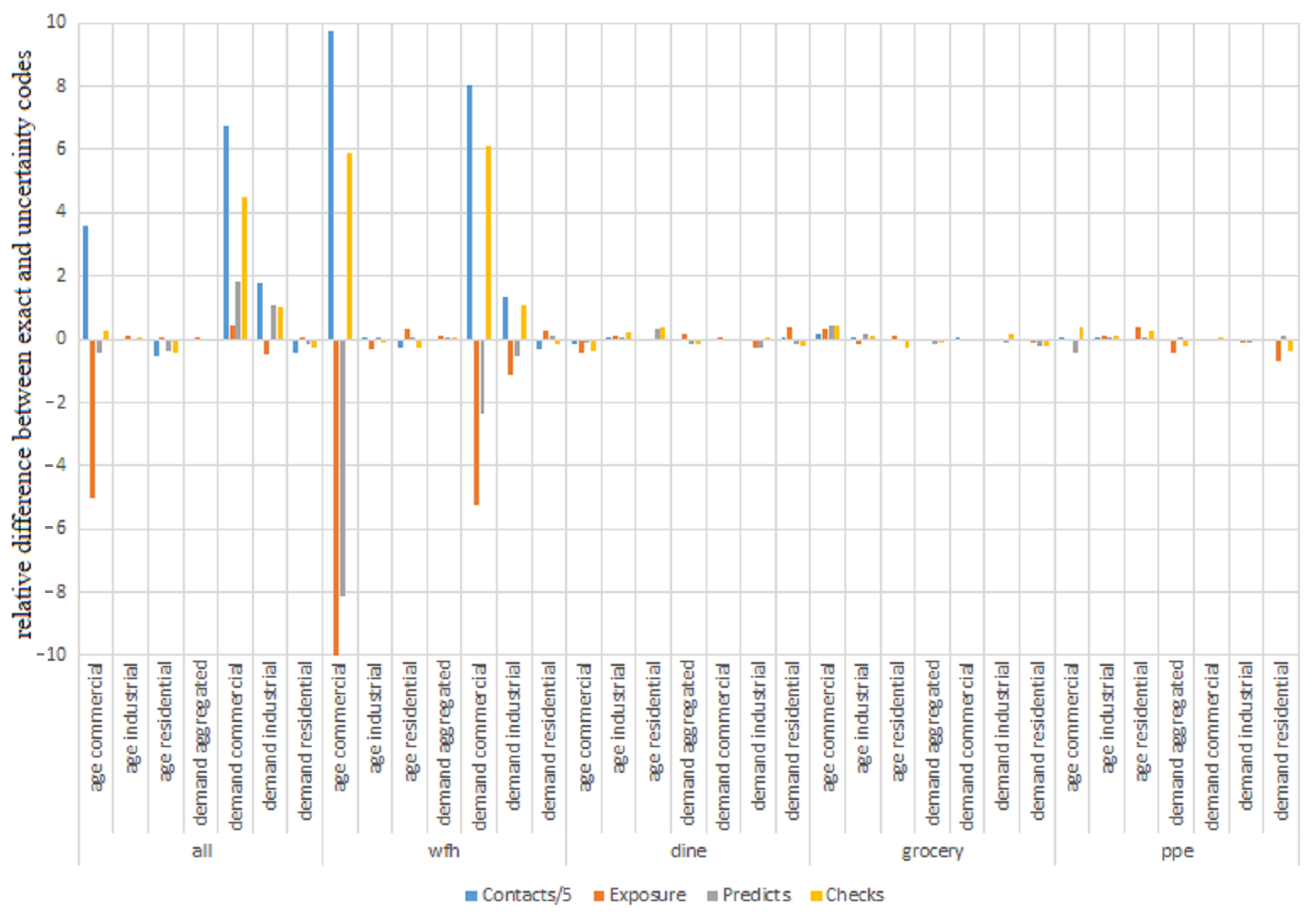
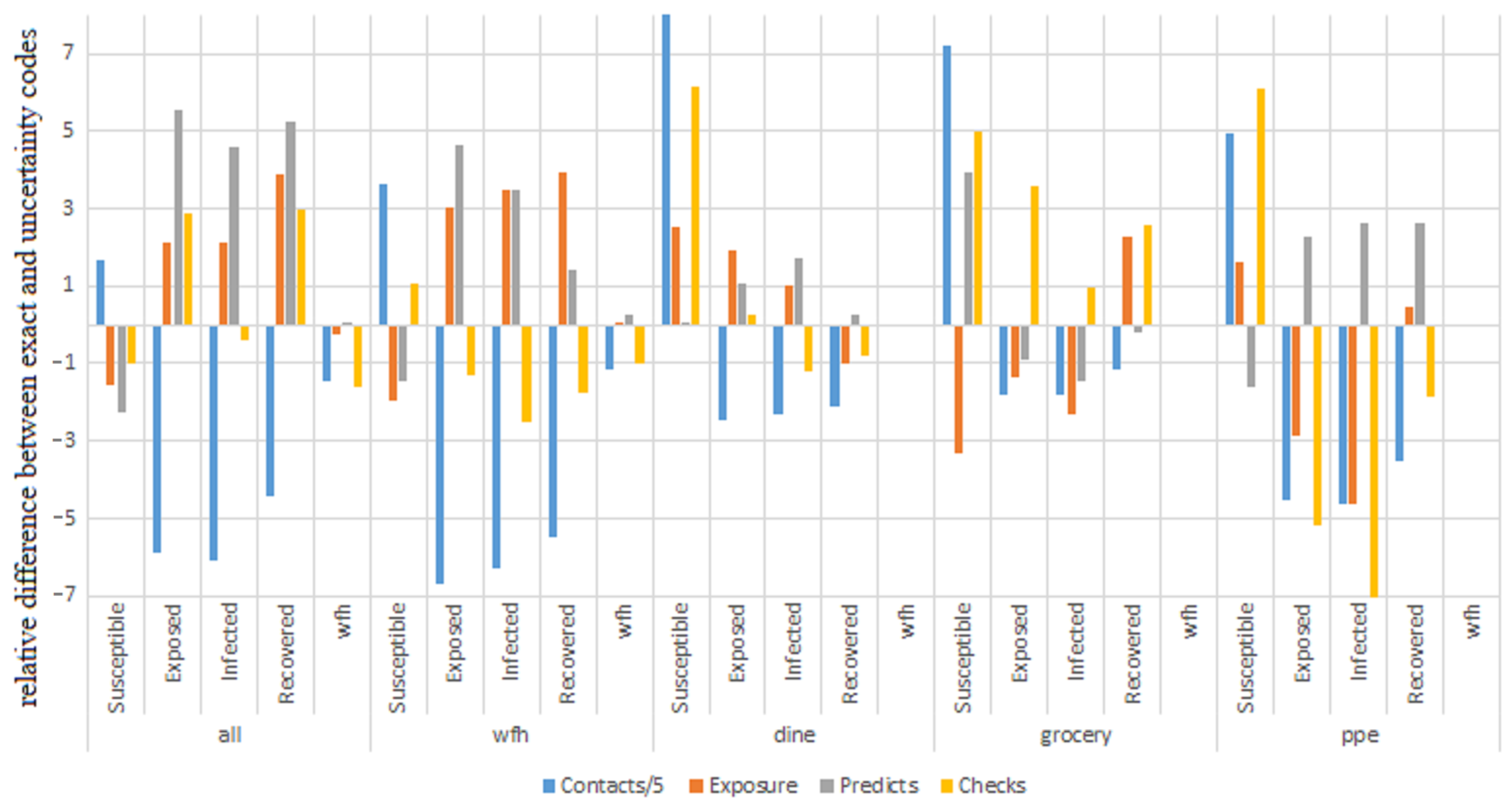
5.1. Sensitivity Analysis of Uncertainty in ABM Parameters

To assess the impact of uncertainty, we compare simulation outcomes using appropriate measures:
  • Age/Demand: Final simulation value difference.
  • Susceptible (S), Recovered (R), and Work-from-Home (wfh) in SEIR: Final value difference.
  • Exposed (E) and Infected (I): Peak difference.
Uncertainty was introduced by applying uniform variations around the original probability, as described in Section 3.4.1. Due to negligible effects at smaller ranges, we compare the original ABM code with an uncertainty range of [0%, 200%] around the original probability (100%). This ensures the original probability remains the mean value, allowing for a fair comparison.
Figure 4 presents SEIR performance measures under different PMs and uncertainty locations in the ABM code. A bar chart format is used for clarity, while detailed numerical comparisons are available in Table A3 in the Appendix A. The bars represent the relative difference (in peaks or final values) between the exact model and the uncertainty-modified model at specific locations in the code. Notably, agent movement parameters exhibit higher variations than other locations. To improve visualization, all agent movement differences have been scaled down by a factor of 5. Figure 4 shows that when scaled evenly, agent contacts have the most significant impact across all prevention measures.
Next, we present a similar bar chart (Figure 5), but instead of SEIR measures, we compare demand and age. As before, the comparison is presented in a bar chart for clarity, with detailed numerical results available in Table A4. Since the values for contacts are significantly higher than those in other locations, they are scaled down by a factor of 5 for better visualization. Figure 5 includes only the work-from-home (“wfh”) and “all” cases, as the differences in other PM scenarios were negligible. However, the full bar chart is available in the Appendix A (Figure A1). Similar to the previous figure, when scaled evenly, agent contacts have the largest effect. Additionally, we observe a strong impact of other PMs at commercial nodes, influencing both age and demand. Next, we analyze the emergence observed in these figures.

Analysis

Table A3 shows that in SEIR results, the “wfh” column remains zero for all PM scenarios except the “wfh” case. This is expected, as the work-from-home measure was not applied in the other scenarios (“grocery,” “dine,” and “ppe”). A common effect can be seen across all SEIR results. Figure 6 helps explain why changes in performance measures occur when uncertainty is introduced in the number of daily contact agents.
In the original model (without uncertainty), the number of agents at a specific node, a g e n t s _ a t _ n o d e , is compared to the predefined parameter for daily contacts, d a i l y _ c o n t a c t s . If a g e n t s _ a t _ n o d e exceeds d a i l y _ c o n t a c t s , a random selection of d a i l y _ c o n t a c t s agents is exposed. Otherwise, all agents at the node are exposed. Introducing uncertainty affects this process, leading to variations in exposure rates and subsequent SEIR dynamics.
In the modified code that incorporates uncertainty, we compare a g e n t s _ a t _ n o d e with 2 · d a i l y _ c o n t a c t s .
-
If a g e n t s _ a t _ n o d e is smaller, a random number of agents is selected uniformly from the range [ 0 , a g e n t s _ a t _ n o d e 1 ] to be exposed.
-
Otherwise, a random number of agents is selected uniformly from the range [ 0 , 2 · d a i l y _ c o n t a c t s 1 ] to be exposed.
In the specific case shown in Figure 6, we use d a i l y _ c o n t a c t s = 30 .
Figure 6a illustrates the number of selected agents as a function of the total available agents at the node. Figure 6b presents several simulation outputs, averaged over multiple simulation runs. Specifically, it shows the percentage of infected individuals over the simulation period, with each plot displaying the mean and a standard error band around it. The orange and blue curves compare the original and uncertainty-integrated models, respectively, while the green curve represents the average number of agents per node, considering only commercial and industrial node types.
We observe a fundamental challenge in comparing the original and modified codes, as they do not share the same mean. For instance, when fewer than 60 agents are present at a node, the uncertainty-based model yields a lower mean, whereas above 60 agents, both models exhibit the same mean. As a result, the final number of selected agents is not directly comparable. This distinction makes d a i l y _ c o n t a c t s different from other uncertainty sources, as its mean differs. This effect is evident in Figure 6b, where around 60 agents per node (on average) correspond to the vertical dotted line crossing the green curve. At this threshold, the orange and blue curves begin to diverge, illustrating the impact of the differing mean values. Since fewer than 60 available agents lead to a lower selection count in the uncertainty-based model, the infected percentage is reduced. Another possible explanation for this decrease is a lower exposure rate due to reduced social interactions and media exposure.
A decrease in the number of infected individuals (I) results in more people remaining in the susceptible category (S), as fewer daily contacts limit exposure. Alternatively, following Vizanko et al. [14], where deceased individuals are excluded from the model (with minimal numbers per thousand), if I decreases, then E and S increase while maintaining the conservation law S + R = 1 (neglecting the deceased). Given enough simulation time, most infected individuals eventually recover. At any moment, S + E + I + R = 1 , ensuring that every agent is in one of these states. Additionally, Table A4 highlights that in the “wfh” and “all” cases (per Vizanko et al. [14]), the most significant impact on age distribution occurs in these scenarios. For the remaining PMs, age and demand remain relatively constant. Ultimately, our results indicate that the system is resilient to the introduced uncertainty, likely because it applies uncertainty to an already uncertain system.

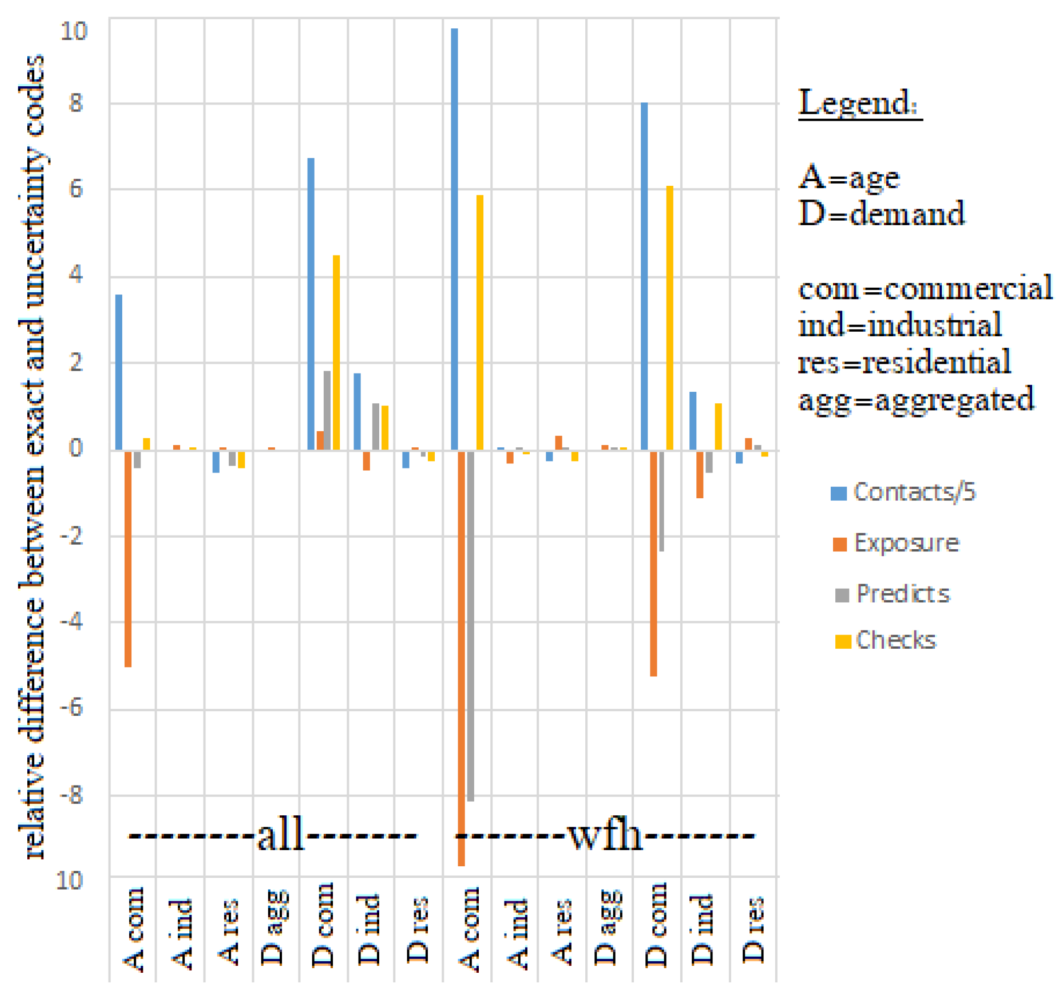
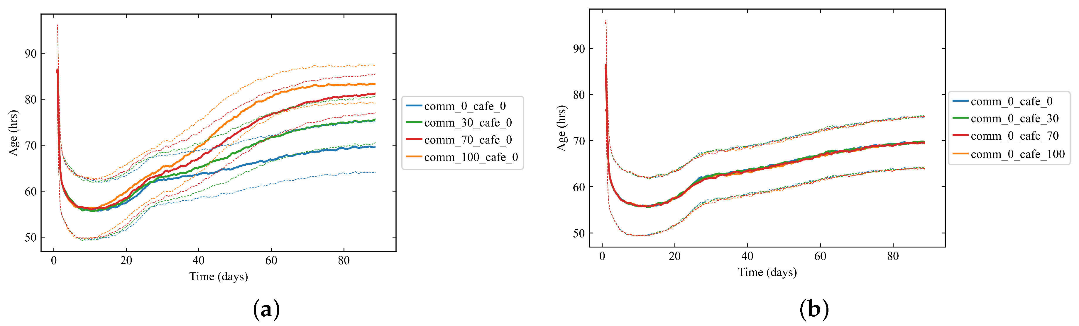
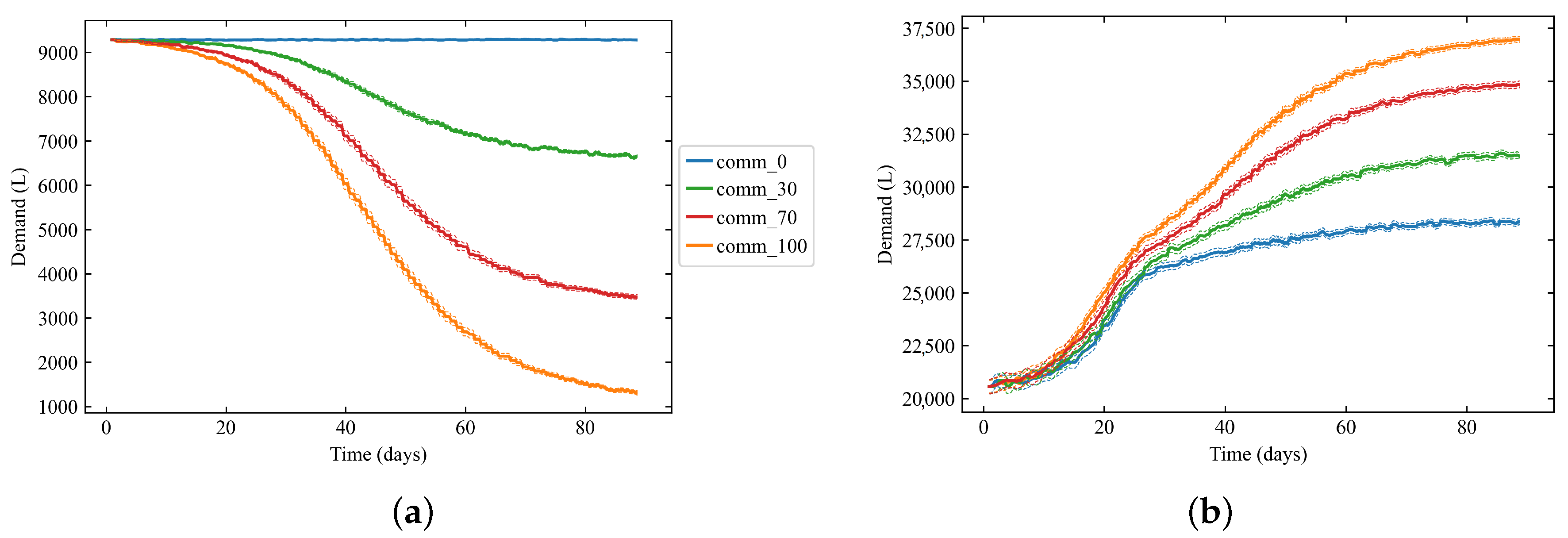
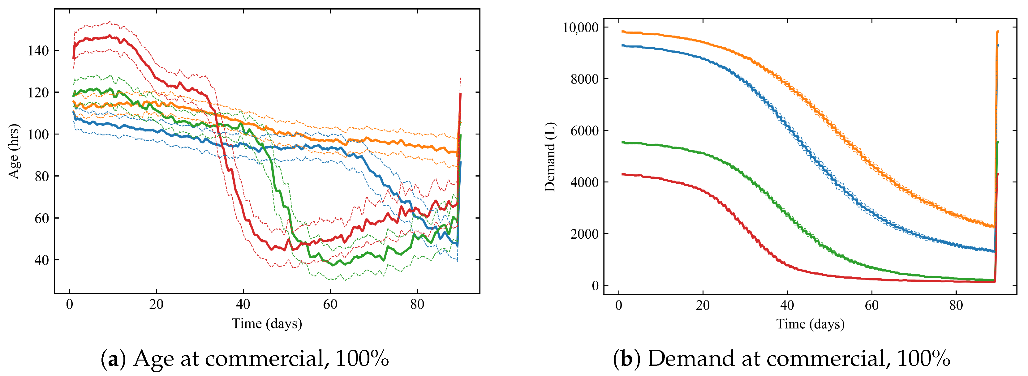
5.2. Adding Non-Workers to Commercial and Café Nodes

Another method for analyzing uncertainty involved modifying agent movement patterns. Figure 7 illustrates a water network with different node types (distinguished by colors). It depicts both the previous scenario, where only workers move from residential to commercial nodes, and the updated scenario, which allows non-workers to move from residential to commercial nodes (represented by the brown arrows). In the original model, agents moved between nodes only when required, always including residential nodes in their movement. In residential⟷industrial transitions, half of the total agents working in industrial nodes return home, while an equal number of new agents begin their shift. If the work-from-home (wfh) policy applies, the affected agents remain in their residential nodes rather than commuting.
Previously, only workers commuting for employment traveled to commercial nodes, and all agents could return to their residential nodes. However, in the modified scenario, a predefined percentage of non-workers are also allowed to move from residential to commercial nodes. A lower percentage parameter results in more non-workers traveling to commercial nodes, increasing the total number of agents and, consequently, demand at commercial locations. This shift slightly affects the number of wfh agents, as increased commercial activity leads to higher infection rates, triggering more work-from-home decisions through Bayesian Belief Network (BBN) modeling. Despite this, the overall demand remains nearly constant, implying fewer agents in residential nodes. However, the number of agents per node in industrial zones remains unchanged. We hypothesize that this occurs because wfh adoption remains minimal, preserving the steady transfer rate of agents between residential and industrial nodes.
Figure 8 presents aggregated age plots, representing the total age across all node types (commercial, industrial, and residential). It explores two cases: Figure 8a examines a scenario where the movement of agents to cafés is fixed, while the distribution of commercial agents varies. Conversely, Figure 8b maintains a fixed commercial agent distribution while modifying the movement of agents to cafés. Each subplot includes four cases corresponding to different agent distribution patterns. As observed in Figure 8, modifying café percentages while keeping commercial percentages constant has little to no impact. However, the opposite scenario—fixing café percentages and adjusting commercial percentages—produces noticeable changes in the results. This disparity arises because there are significantly fewer café nodes than commercial nodes. Consequently, the number of agents at café nodes is much lower than at commercial nodes. Thus, variations in café movement percentages translate to a small number of affected agents, insufficient to influence the final outcomes.

Demand Analysis for Varying Commercial Percentages

After establishing that adjusting café percentages has negligible effects on various measures, we focus on the impact of commercial agent percentages. Specifically, we analyze demand variations. Figure 9 presents these results, mirroring the conditions in Figure 8b, where the café distribution remains fixed at 30%, while the commercial distribution varies from 0% (no working) to 100% (only working). Unlike Figure 8, which aggregates results, Figure 9 presents separate demand plots: Figure 9a illustrates demand in the commercial sector, while Figure 9b focuses on demand in the residential sector.
Figure 9 demonstrates the effect of increasing the proportion of working agents moving from residential to commercial nodes. Higher movement percentages (e.g., 100%) indicate that more agents attempt to commute to commercial nodes. However, under the Bayesian Belief Network (BBN) model, these agents are more likely to choose to stay home and work remotely to minimize COVID-19 exposure. As a result, demand at commercial nodes decreases over time, while demand at residential nodes rises. Conversely, when fewer agents intend to commute to commercial nodes for work (lower movement percentages, e.g., 0%), more agents travel to commercial nodes regardless of COVID-19 considerations. This outcome aligns with the structure of the ABM framework, where agent movement is predefined. Although not explicitly depicted, industrial nodes remain unaffected by variations in working agent percentages shifting from residential to commercial nodes. This stability occurs because industrial workplaces follow fixed shift exchanges, irrespective of changes in commercial movement dynamics.

5.3. Changing the Distribution of Agents in the Network

We conducted experiments to explore how the distribution of agents across the network affects outcomes. To ensure a fair comparison, we maintained a similar total agent capacity across all nodes while varying the distribution of agents among different node types.

Scenarios for Different Distributions

The selected distributions reflect realistic scenarios. The same rule applies: no agents are assigned to non-residential nodes at night, except for industrial nodes with night shifts. We kept the agent count stable in cafés and commercial nodes. The distribution was primarily based on the number of agents in industrial nodes, redistributing them between industrial and other node types.
In the following, we describe the scenarios for different distributions, and then present in Table 2 the time-averaged agent capacity distributions accross different node types for each of these scenarios.
  • Less-ind: Fewer agents in industrial nodes, leading to an increase in cafés, commercial, and, especially, residential nodes.
  • Regular: The default distribution, representing a typical city.
  • More-ind: More agents in industrial nodes, resulting in fewer in cafés, commercial, and residential areas, resembling an industrial town.
  • Much-more-ind: A heavily industrialized area designed primarily for work, with minimal residential accommodations.
Figure 10 and Figure 11 depict age and demand variations for different distributions. Figure 10 presents results for 100% and 30% of agents moving to commercial nodes, while Figure 11 focuses on the industrial sector at 100%. As industrial presence increases, fewer agents visit commercial nodes, opting to work from home. This results in a significant decrease in water age. Interestingly, Figure 10 shows that demand also declines, despite typically having an inverse relationship with water age. This trend is observed at both 100% and 30% worker movement levels. However, in the industrial sector, demand and water age follow the expected inverse correlation, as shown in Figure 11. A possible explanation is that commercial nodes are centrally located in our water network (Micropolis). The main water supply first passes through commercial nodes before reaching industrial areas. High demand in the bottom right of the network, coupled with low demand in commercial areas, leads to a lower-than-expected water age at commercial nodes. This is due to significant flow driven by downstream residential demand. This effect is specific to the given network configuration. Variability in agent distribution results in nonlinear and unpredictable outcomes due to complex interactions within different networks.

6. Discussion

6.1. Results Discussion

Most of the results presented in Section 5.1 align with expectations and are predictable, even in cases where differences are observed, such as daily contacts. This is because the ABM for WDS was intentionally designed to exhibit robust behavior, even under increasing uncertainty in parameter selection. Additionally, the observed variations are likely due to the introduction of uncertainty into an already uncertainty-embedded model. In the case of daily contacts, it may initially appear that uncertainty introduces some effects. However, upon further analysis, these effects are attributed to differences in mean comparisons rather than actual behavioral changes. Overall, the ABM system demonstrates resilience, even under scenarios where increased uncertainty is applied to its parameters.
Significant effects were primarily observed in cases where uncertainty was not originally embedded. These include the movement of non-workers to commercial and café nodes (Section 5.2) and changes in agent distribution across the network (Section 5.3). The most pronounced effects were seen in the movement of non-working agents to commercial nodes, primarily because their numbers far exceeded those moving to café nodes. Consequently, we focused more on analyzing agent movement to commercial nodes. The key observation was that agents intending to work remained at home when the work-from-home (WFH) policy was applied, leading to lower demand at commercial nodes. Conversely, agents moving for non-work purposes were unaffected by WFH policies, resulting in increased movement to commercial nodes and a higher COVID-19 transmission risk. This, in turn, increased demand at commercial nodes. In all cases, demand in residential nodes complemented that in commercial nodes, assuming no changes in residential⟷industrial movement patterns. When analyzing the impact of changing agent distribution by node type (Section 5.3), we found the outcomes to be more challenging to explain due to the network’s complex, nonlinear interactions. The spatial distribution of nodes within the network plays a crucial role, making predictions difficult.
It is important to note that all uncertainty scenarios were designed to mimic realistic conditions. For example, it is reasonable to assume that agents move to commercial nodes not only for work but also for shopping. Similarly, changing agent distributions within the network represents different types of cities—some being more industrial while others more commercial or more residential. While other uncertainty cases could be explored, their practical relevance to real-world WDSs is not guaranteed.
In Section 5.2, when examining the uncertainty effects in the movement of non-workers to commercial and café nodes, we found that the greatest impact occurred when agents moved to commercial nodes. This is due to the significantly larger number of agents in commercial nodes compared to café nodes. Furthermore, WDS performance is highly dependent on the configuration of the infrastructure, particularly when uncertainty is introduced into the distribution of agent types within the network.

6.2. Emergence in Complex Systems

Water distribution systems function as sociotechnical systems, where interactions between human behavior and infrastructure influence system performance. Changes in customer demand directly impact infrastructure behavior, sometimes leading to system transitions that are unpredictable or unexpected due to dynamic feedback loops and adaptive behaviors. Emergence refers to system-level behaviors, structures, or patterns that are not explicitly programmed but arise due to network interactions among agents and their environment [28]. Emergence is classified into four categories, as defined by [29]: simple, weak, strong, and spooky emergence. Simple and weak emergence can be predicted and reproduced using simplified models. Strong emergence, in contrast, cannot be replicated by simplifications of the system. Spooky emergence, the most unpredictable form, does not appear in any model, even when simulating the full system with all details. ABM has been applied to WDSs to provide new insights into system management. It enables capturing emergent phenomena that would be difficult or impossible to predict. For example, during a water contamination event, interactions between agents can cause shifts in water demand that alter flow directions, exposing different populations to contaminants [11]. By analyzing infrastructure through the interactions between technical and social systems, we gain a better understanding of performance changes under different conditions.
In this study, we introduced uncertainty into the ABM to simulate water quality changes in a small virtual hydraulic network, leading to emergent behavior. We found that water demand and age remained robust despite uncertainty in COVID-19 transmission parameters. However, emergent behavior was observed when we modulated the number of agents moving for work and the total number of workers present in the network. The primary objective of this research was to analyze the effects of uncertainty, rather than directly studying emergence in a methodological sense. However, future research could explore potential connections between uncertainty and emergent behavior.

6.3. Applicability to Real-World Systems

While the Micropolis testbed provides a convenient, controlled environment for isolating the effects of behavioral uncertainty, real utilities face additional challenges that may influence the performance of our ABM–WNTR coupling. Actual networks exhibit a far larger scale, more complex topology, variable pipe aging and roughness, and heterogeneous meter-data quality. Moreover, obtaining reliable socio-behavioral inputs—such as time-use surveys, mobile-phone movement data, or localized media-exposure rates—can be difficult and may require partnerships with academic or municipal data providers. To adapt our methodology, practitioners should begin by calibrating the ABM to local demand traces (e.g., smart-meter records) and validating predicted shift patterns (e.g., work-from-home rates) against observed billing or telemetry data. Network modelers should also carry out a preliminary sensitivity screening on hydraulic parameters (roughness, demand patterns) to ensure the ABM-driven variations propagate meaningfully through their specific infrastructure. Finally, because large-scale coupled simulations can be computationally intensive, we recommend an iterative approach: (1) pilot runs on key sub-areas or critical zones, (2) refinement of the behavioral model through stakeholder feedback, and (3) gradual scaling to the full network. By following these steps, utilities can leverage our uncertainty framework to improve preparedness for demand-shifting events—whether pandemics, mass gatherings, or extreme weather—while managing the practical constraints of real-world data and computation.

7. Conclusions

As an extension of previous research Vizanko et al. [14], this paper aimed to analyze the ABM framework under different uncertainty scenarios, specifically in the COVID-19 transmission model, worker mobility, and node-type distribution of agents. We employed different methods to introduce uncertainty. In the COVID-19 transmission model, we incorporated uncertainty by varying the thresholds within the ABM code. For worker mobility, we defined a new random variable to distribute agents’ movements between residential, commercial, and café nodes based on working and non-working purposes. In the node-type distribution, we applied different random distributions of a fixed total number of agents across node types to represent uncertainty in agent distribution within the network.
Our results demonstrate that the ABM system is robust when uncertainty is applied to COVID-19 transmission parameters, which already possess an inherent probabilistic nature. However, introducing uncertainty in agent movement led to significant changes in system behavior, particularly in scenarios involving non-working agents moving to commercial nodes. Further analysis revealed that agents intending to work tended to stay home when the work-from-home (wfh) policy measure was applied, leading to decreased demand at commercial nodes. Conversely, agents moving for non-working purposes were unaffected by this policy, increasing demand at commercial nodes and potentially elevating COVID-19 transmission risks. Additionally, modifying agent distribution across node types produced varied effects—some expected, others unexpected. Further examination suggested that these outcomes resulted from complex interactions within the specific network structure.
In summary, the system exhibits robustness when uncertainty is applied to already probabilistic parameters. However, uncertainty in agent movement has a significant impact. Finally, different agent distributions, simulating various city types, exhibited surprising and non-linear network-dependent effects. Future research could explore additional uncertainty scenarios and potential emergence effects.

Author Contributions

Conceptualization, S.K. and B.V.; methodology, S.K. and B.V.; software, S.K. and B.V.; validation, S.K. and B.V.; formal analysis, S.K. and B.V.; investigation, S.K. and B.V.; resources, S.K. and B.V.; data curation, S.K. and B.V.; writing—original draft preparation, S.K., B.V., E.B., and A.O.; writing—review and editing, S.K., B.V., E.B., and A.O.; visualization, S.K. and B.V.; supervision, E.B. and A.O.; project administration, E.B. and A.O.; funding acquisition, E.B. and A.O. All authors have read and agreed to the published version of the manuscript.

Funding

This research received no external funding.

Data Availability Statement

All data, models, and code that support the findings of this study are available from the corresponding author upon reasonable request. The ABM is available through Zenodo at 10.5281/zenodo.10277434.

Acknowledgments

This research was funded by the United States—Binational Science Foundation (BSF). We would also like to thank both the City of Lakewood and [30] for providing access to data that were critical to the development of the models presented in this research.

Conflicts of Interest

The authors declare no conflicts of interest.

Appendix A

The experiments of uncertainty in SEIR, conducted firstly in random seeds of batch of simulations.
Table A1. Comparison of different performance measures for different performance measures (columns) and uncertainty locations in ABM code (rows).
(a)
Exact vs.allwfh
Contacts10.87−35.10−36.44−28.82−11.7316.06−31.95−29.37−27.45−7.12
Exposure−3.065.153.678.992.181.94−7.89−4.26−7.22−3.00
Predicts−1.597.042.897.491.89−0.06−0.480.78−2.900.57
Checks−0.06−1.88−5.431.31−0.10−2.00−0.56−0.970.04−0.51
(b)
Exact vs.dinegrocery
Contacts43.17−14.71−13.14−11.27089.83−15.66−15.36−15.870
Exposure2.84−6.08−4.92−3.1105.44−4.00−3.50−2.780
Predicts−4.521.901.831.7002.66−4.32−3.47−3.530
Checks6.69−0.66−2.38−1.13012.62−6.49−7.42−4.360
(c)
Exact vs.ppe
Contacts20.56−17.83−16.93−15.020
Exposure−3.835.613.696.540
Predicts-4.638.086.247.480
Checks0.060.55−2.183.270
In Table A2, due to randomness, some of the results have different means, while in the organized ones, the mean is always the same. It takes even few simulations to produce different means (because we see that the means are very close). We find irregularities where the agents are being placed due to random seeds, which produce different agent distributions among the nodes.
Table A2. Comparison of demand and age by different performance measures (columns) and uncertainty locations in ABM code (rows).
(a)
Exact vs.allwfh
Contacts29.680.68−3.33−0.9252.609.70−3.7567.30−0.52−3.440.7262.5617.39−1.68
Exposure−9.72−0.16−0.61−0.39−7.042.49−0.1720.26−1.03−2.510.5130.5213.89−0.81
Predicts−15.51−0.82−0.030.17−10.661.480.6210.380.260.15−0.085.341.68−0.30
Checks1.260.00−0.34−0.591.272.33−0.776.97−0.26−1.600.317.3411.16−0.23
(b)
Exact vs.dinegrocery
Contacts−0.45−0.96−3.071.58−0.05−0.052.67−2.11−0.49−0.371.61−0.03−0.142.71
Exposure−1.70−0.49−1.921.580.00−0.062.640.550.060.77−0.480.03−0.27−0.74
Predicts−3.04−0.48−1.002.82−0.02−0.104.731.330.28−0.11−1.75−0.04−0.01−2.88
Checks−1.24−1.16−1.742.11−0.020.073.51−2.75−0.84−2.922.91−0.04−0.044.85
(c)
Exact vs.ppe
Contacts−1.86−0.90−2.182.76−0.010.114.65
Exposure−1.67−0.63−1.342.38−0.02−0.054.05
Predicts−1.54−1.13−2.563.630.00−0.256.20
Checks−1.61−1.18−3.483.560.010.036.01
Subsequently, we performed the same analysis only on organized seeds as explained in Section 5.1.
Table A3. Comparison of SEIR by different performance measures for different PMs (columns) and uncertainty locations in ABM code (rows).
(a)
Exact vs.allwfh
Contacts8.26−29.37−30.54−22.24−7.3218.14−33.56−31.34−27.43−5.65
Exposure−1.532.122.113.90−0.27−1.973.013.473.910.03
Predicts−2.275.524.615.260.04−1.474.623.471.410.28
Checks−0.982.86−0.422.97−1.621.04−1.32−2.49−1.74−0.99
(b)
Exact vs.dinegrocery
Contacts41.92−12.33−11.66−10.65036.00−8.95−9.01−5.840
Exposure2.521.931.02−0.990−3.32−1.36−2.332.270
Predicts0.021.041.700.2403.92−0.88−1.47−0.210
Checks6.150.25−1.21−0.8105.013.560.952.560
(c)
Exact vs.ppe
Contacts24.81−22.72−23.03−17.560
Exposure1.64−2.88−4.600.440
Predicts−1.592.252.632.620
Checks6.11−5.20−7.29−1.880
The inner columns for each PM scenario are as follows: 1 = Susceptible; 02 = Exposed; 03 = Infected; 04 = Recovered; 05 = wfh = work from home. The rows represent the difference in some measure between the exact code and the code with uncertainty in a specific location in the code. The values in the SEIR table are the relative difference (either in peaks or in final values).
Next, we present a similar table, only that the results are for demands and age instead of SEIR.
The inner columns for each PM scenario are as follows: 01 = age, sector: Commercial; 02 = age, sector: Industrial; 03 = age, sector: Residential; 04 = demand, aggregated; 05 = demand, section: Commercial; 06 = demand, section: Industrial; 07 = demand, section: Residential.
The rows represent the difference in some measure between the exact code and the code with uncertainty in a specific location in the code. The values in Table A4 are the average of the final values.
We also add a bar chart corresponding to Table A4 for a better visualization of the data.
Table A4. Comparison of demand and age by different performance measures for different PMs (columns) and uncertainty locations in ABM code (rows).
(a)
Exact vs.allwfh
Contacts17.89−0.30−2.52−0.3233.868.74−2.1848.670.14−1.35−0.1440.046.60−1.61
Exposure−5.050.120.050.030.42−0.470.02−11.72−0.310.330.09−5.23−1.140.29
Predicts−0.45−0.02−0.36−0.021.821.08−0.14−8.110.040.010.01−2.36−0.520.10
Checks0.290.04−0.42−0.024.491.01−0.265.88−0.09−0.240.046.081.07−0.18
(b)
Exact vs.dinegrocery
Contacts−0.710.02−0.34−0.010.00−0.100.010.730.11−0.32−0.070.03−0.03−0.12
Exposure−0.400.11−0.040.180.01−0.280.360.30−0.180.09−0.07−0.05−0.01−0.09
Predicts−0.080.050.34−0.15−0.03−0.28−0.180.420.16−0.07−0.150.00−0.11−0.23
Checks−0.350.230.40−0.15−0.070.01−0.220.430.12−0.26−0.12−0.020.19−0.23
(c)
Exact vs.ppe
Contacts0.170.14−0.07−0.11−0.05−0.05−0.14
Exposure−0.040.110.36−0.440.00−0.10−0.71
Predicts−0.400.070.010.04−0.01−0.100.10
Checks0.370.090.27−0.220.03−0.01−0.38
Figure A1. Comparison of SEIR by different performance measures for different PMs and uncertainty locations in ABM code. We use final value differences.
Water 17 01965 g0a1

Appendix B. Process Scheduling Details

The following descriptions for Steps H1–H5 and D1–D5 are adapted from Vizanko et al. [14].
Step H1.
Agents move between residential and non-residential nodes. Agents move between nodes based on predefined node capacities and node type requirements. Agents are assigned to move to and from non-residential nodes based on an hourly total capacity at each non-residential node.
Step H2.
Agents update COVID-19 status indicators. Agents update COVID-19 status indicators, which represent the number of hours an agent spends in the exposed, infected, severe, and symptomatic stages ( t e x p , t i n f , t s e v , and t s y m p , respectively).
Step H3.
Agents transmit COVID-19. Infected agents expose susceptible agents when they occupy the same node. When an infected agent moves to a new node, up to 10 susceptible agents at the new node are exposed based on the node’s exposure rate ( e r e s for residential nodes, e n r for non-residential nodes in Table A5).
Step H4.
Agents update mass media exposure. Agents receive information from TV and radio based on probabilistic estimates that they use each form of media at each hour of the day [11,31] (Table A8). The mass media exposure ( C m e d ) is a binary number that is changed from 0 to 1 once an agent receives information about COVID-19 at any time step, based on probabilistic behaviors to use radio and TV.
Step H5.
Agents exert water demand. The hourly demand at each node is calculated based on the number of agents at each node as follows:
B d t , N = K N K N , c a p × B d t , N
where B d t , N is the new demand for node N at time t, K N is the number of agents at node N, K N , c a p is the capacity of node N, and B d t , N is the base demand.
The following steps are completed every 24 h:
Step D1.
Agents update COVID-19 status. Agents update COVID-19 status state variables (S, S s y m p , and S i n f ) based on their progression through disease stages. Once the time in a stage exceeds an agent’s threshold for that stage (e.g., t e x p > τ e x p , Table A5), the agent updates its COVID-19 status (e.g., S = i n f e c t e d ).
Step D2.
Agents update personal experience with COVID-19. Once an agent enters the infectious stage ( S = i n f e c t e d ), the agent updates the personal COVID-19 status ( C p e r ) from “no” (value of 1) to “doctor confirmed and am still infected” (value of 9) [14].
Step D3.
Agents update friends and family COVID-19 status. An agent updates the friends and family COVID-19 status ( C f f ) when a peer agent enters the infectious stage. The value ( C f f ) can increase up to 7 to represent the number of peers in an agent’s network that are infected. A value of seven corresponds to survey responses that the person is “very much affected” by friends or family testing positive or dying from COVID-19 [14].
Step D4.
Agents update decision to adopt prevention measures. BBN models are applied to calculate the probability of adopting each prevention measure based on mass media exposure, personal COVID-19 status, and friends and family COVID-19 status ( C m e d , C f f , and C p e r , respectively). Prevention measures include working from home, dining out less, grocery shopping less, and wearing PPE, and bottled-water-buying behaviors are drinking bottled water, cooking with bottled water, and using bottled water for hygiene. Refer to previous work for more information on prevention measures [14,32].
Step D5.
Agents update demand patterns. Agents that choose to work from home, dine out less, or grocery-shop less update their demand patterns from a typical diurnal pattern to a pattern that expresses demands uniformly across daylight hours (standard and COVID-19 demand patterns in Table A7).
The last step of the framework is completed at the end of the 90-day period.
Step S1.
Calculate hydraulic performance of the water distribution system. The unique demand patterns reporting the demands at each node and each hour for the 90-day period are passed to the EPANET simulation using WNTR. Results from the hydraulic simulation for each hourly time step are recorded, including the water age and pressure at each node and the flow rate and direction of flow in each pipe.

Appendix C. State Variables and Parameters

The following is taken from Vizanko et al. [14].
Table A5. Agent parameters are used to model exposure to COVID-19, communication, and mobility in the network. LN( x , y ) represents a log-normal distribution with mean x and standard deviation y.
ParameterSymbolValue
Residential exposure rate e r e s 0.05   1
Non-residential exposure rate e n r 0.01   1
Probability of listening to radio P R Table A8
Probability of watching TV P T V Table A8
Work node N w o r k All industrial nodes
Home node N h o m e All residential nodes
Exposed stage threshold (days) τ e x p ∼ LN ( 4.5 , 1.5 ) 1
Symptomatic stage threshold (days) τ s y m p ∼ LN ( 1.1 , 0.9 )   (to severe stage) 1
∼ LN ( 8.0 , 2.0 )   (to recovered stage) 1
Infected stage threshold (days) τ i n f t s y m p + t s e v + t c r i t
Severe stage threshold (days) τ s e v ∼ LN ( 1.5 , 2.0 )   (to critical stage) 1
∼ LN ( 18.1 , 6.3 )   (to recovered stage) 1
Critical stage threshold (days) τ c r i t ∼ LN ( 10.7 , 4.8 )   (to dead stage) 1
∼ LN ( 18.1 , 6.3 )   (to recovered stage) 1
Note: 1 values reported by Kerr et al. [5].
Table A6. Agent state variables.
State VariableSymbolValue
COVID-19 statusS[susceptible, exposed, infected, recovered, dead]
Symptomatic status S s y m p [Symptomatic, asymptomatic]
Infected status S i n f [mild, severe, critical]
Personal COVID-19 status (BBN input) C p e r [ 1 , 9 ]
Friends and Family COVID-19 status (BBN input) C f f [ 1 , 2 , 3 , 4 , 5 , 6 , 7 ]
Mass media exposure (BBN input) C m e d { 0 , 1 }
Time in exposed stage (days) t e x p
Time in symptomatic stage (days) t s y m p
Time in infected stage (days) t i n f
Time in severe stage (days) t s e v
Time in critical stage (days) t c r i t
WFH decision D W F H [Not WFH, WFH]
Dine out less decision D d i n e [Dine out, dine out less]
Grocery shop less decision D s h o p [Grocery shop, grocery shop less]
PPE decision D P P E [Wear PPE, not wear PPE]

Appendix D. Supplemental Information

All the below is taken from Vizanko et al. [14].

Appendix D.1. Daily Demand Patterns

Table A7. Residential demand patterns.
HourStandard Residential PatternCOVID-19 Residential Pattern
00.550.51
10.550.41
20.580.40
30.670.47
40.850.67
51.050.99
61.161.07
71.121.05
81.151.13
91.101.21
101.021.26
111.001.31
121.021.28
131.101.22
141.201.14
151.351.11
161.451.15
171.501.21
181.501.25
191.351.32
201.001.21
210.801.06
220.700.88
230.600.67

Appendix D.2. TV and Radio Probabilities

Table A8. Probabilities of an agent receiving information from radio ( P R ) and TV ( P T V ) for each hour of a given day.
Daily Time Step P R P TV
00.4634.626
10.5770.439
20.350.226
30.350.215
40.5750.006
58.3420.366
620.764.405
724.79417.15
84.43612.898
94.5978.847
100.520.343
114.490.22
128.5154.846
138.6220.151
148.6780.421
1512.7110.656
1612.3280.869
178.25115.769
184.16521.366
190.24317.037
200.3527.649
210.34235.729
220.12331.951
230.2339.203

Appendix D.3. BBN Figures and Tables
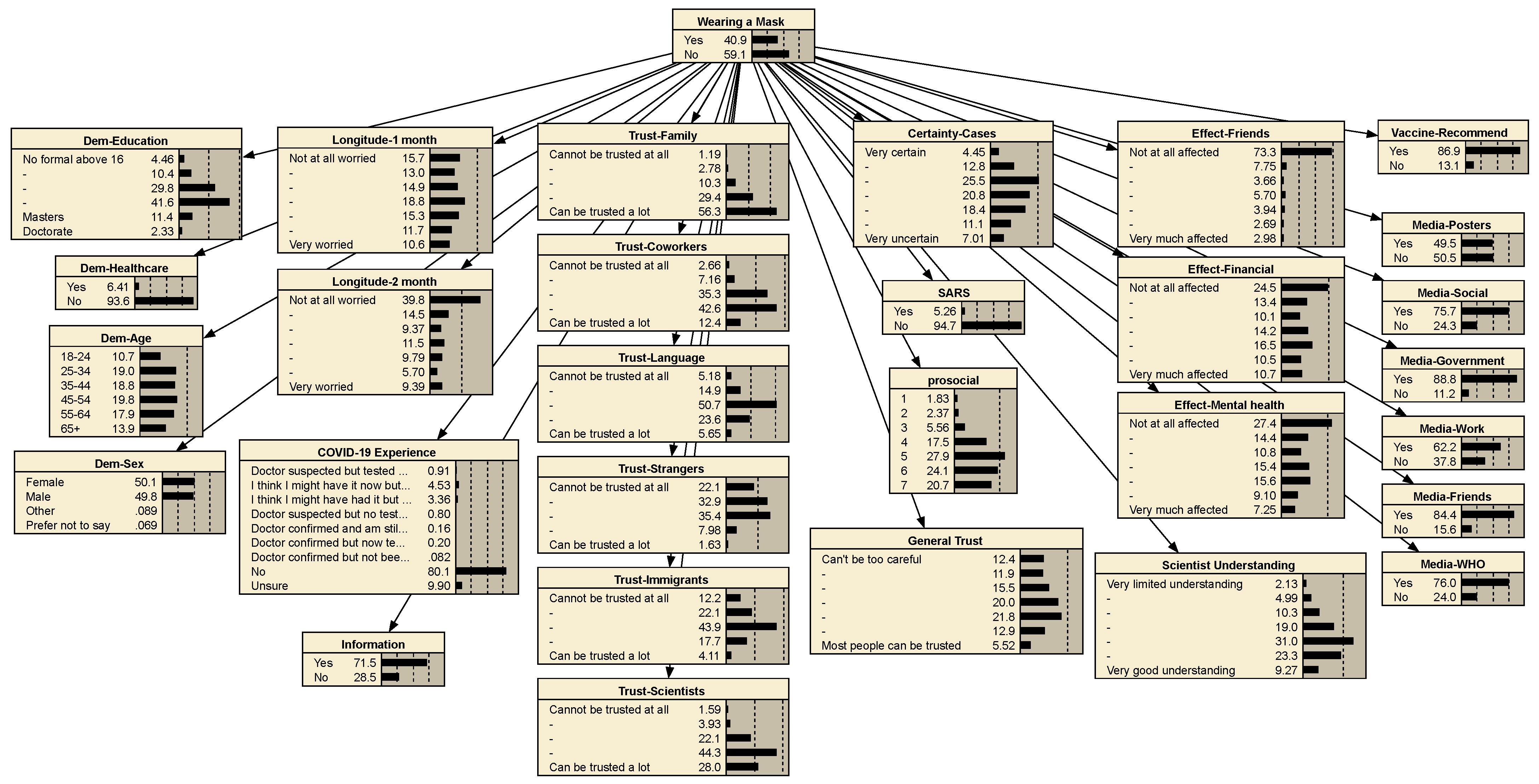
Figure A2. The BBN model is used in agent decision-making to select working from home. The model includes demographic and perception variables.
Water 17 01965 g0a2
Figure A3. BBN model is used to in agent decision-making to select dining out less. Model includes demographic, perception, and PMT variables.
Water 17 01965 g0a3
Figure A4. The BBN model is used in agent decision-making to select grocery shopping less. The model includes demographic, perception, and PMT variables.
Water 17 01965 g0a4
Figure A5. The BBN model is used in agent decision-making to select wearing a mask. The model includes demographic and perception variables.
Water 17 01965 g0a5
Table A9. Variables used as input to the BBN model include demographics, perceptions, and PMT constructs. Question responses are included in the question column in brackets, and Likert scale.
VariableQuestion
Trust-FamilyHow much do you trust people in your family? [5]
Trust-NeighborsHow much do you trust people in your neighbourhood? [5]
Trust-CoworkersHow much do you trust people you work or study with? [5]
Trust-LanguageHow much do you trust people who speak a different language from you? [5]
Trust-StrangersHow much do you trust strangers? [5]
Trust-ImmigrantsHow much do you trust immigrants? [5]
Trust-Medical staffHow much do you trust medical doctors and nurses? [5]
Trust-ScientistsHow much do you trust scientists? [5]
Media-PostersHave you come across information about coronavirus or COVID-19 from: official public posters. [1: yes, 2: no]
Media-SocialHave you come across information about coronavirus or COVID-19 from: social media or online blogs from individuals. [1: yes, 2: no]
Media-JournalistHave you come across information about coronavirus or COVID-19 from: journalists and commentators in the media (TV, radio, newspapers). [1: yes, 2: no]
Media-GovernmentHave you come across information about coronavirus or COVID-19 from: government or official sources such as websites or public speeches/broadcasts within the country you are living in. [1: yes, 2: no]
Media-WorkHave you come across information about coronavirus or COVID-19 from: official messages from your place of work or education. [1: yes, 2: no]
Media-FriendsHave you come across information about coronavirus or COVID-19 from: friends and family. [1: yes, 2: no]
Media-WHOHave you come across information about coronavirus or COVID-19 from: World Health Organisation. [1: yes, 2: no]
Current Worry-ClimateHow worried are you personally about climate change at present? [7]
Current Worry-ImmigrationHow worried are you personally about immigration at present? [7]
Current Worry-TerrorismHow worried are you personally about terrorism at present? [7]
Current Worry-CrimeHow worried are you personally about crime at present? [7]
Future Worry-FinancesHow likely do you think it is that [you (ps) OR your friends and family in the country you are currently living in (fs)] will be directly affected by financial problems in the next 6 months? [7]
Future Worry-AvoidanceHow likely do you think it is that [you (ps) OR your friends and family in the country you are currently living in (fs)] will be directly affected by antisocial behavior by others in the next 6 months? [7]
Future Worry-ImmigrationHow likely do you think it is that [you (ps) OR your friends and family in the country you are currently living in (fs)] will be directly affected by immigration in the next 6 months? [7]
Dem-SexWhat is your sex? [1: female, 2: male, 3: other, 4: prefer not to say]
Dem-AgeWhat is your age? [1: 18–24, 2: 25–34, 3: 35–44, 4: 45–54, 5: 55–64, 6: 65+]
Dem-HealthcareAre you a healthcare provider (e.g., doctor, nurse, paramedic, pharmacist, carer)?
Dem-EducationPlease indicate your highest educational qualification: [1: no formal above 16 to 5: Masters, 9: doctorate]
Prioritize SocietyTo what extent do you think it’s important to do things for the benefit of others and society even if they have some costs to you personally? [7]
COVID-19 ExperienceHave you ever had, or thought you might have, the coronavirus/COVID-19? [9: unsure, 8: no, 3: I think I might have had it but am recovered, 2: I think I might have it now but not tested, 1: doctor suspected but tested negative, 4: doctor suspected but no test yet, 5: doctor confirmed and am still infected, 6: doctor confirmed but now test negative, 7: doctor confirmed but not been tested again]
Longitude-1 weekHow worried were you about coronavirus 1 week ago? [7]
Longitude-1 monthHow worried were you about coronavirus 1 month ago? [7]
Longitude-2 monthsHow worried were you about coronavirus 2 months ago? [7]
Effect-FinancialTo what extent have you been affected by the coronavirus/COVID-19 in the following ways?— I have experienced financial difficulties as a result of the pandemic [7]
Effect-SocialTo what extent have you been affected by the coronavirus/COVID-19 in the following ways?—I have experienced social difficulties as a result of the pandemic [7]
Effect-Mental healthTo what extent have you been affected by the coronavirus/COVID-19 in the following ways?—I have experienced mental health difficulties as a result of the pandemic (e.g., increased anxiety) [7]
Effect-FriendsTo what extent have you been affected by the coronavirus/COVID-19 in the following ways?—I have friends and family who have tested positive or died from the virus [7]
SARSHave you personally been affected by a previous similar epidemic such as SARS (Severe Acute Respiratory Syndrome), MERS (Middle East Respiratory Syndrome) or Ebola? [1: yes, 2: no]
General TrustGenerally speaking, would you say most people can be trusted, or that you can’t be too careful in dealing with people? [7]
InformationHave you sought out information specifically about coronavirus/COVID-19? [1: yes, 2: no]
Scientist UnderstandingTo what extent do you think scientists have a good understanding of the coronavirus/COVID-19? [7]
Certainty-KnowledgeHow certain or uncertain do you think the following are: The current scientific knowledge about the coronavirus/COVID-19? [7]
Certainty-CasesHow certain or uncertain do you think the following are: The estimates of the number of cases of coronavirus/COVID-19 worldwide [7]
Vaccine-PersonalIf a vaccine were to be available for the coronavirus/COVID-19 now: Would you get vaccinated yourself? [1: yes, 2: no]
Vaccine-RecommendIf a vaccine were to be available for the coronavirus/COVID-19 now: Would you recommend vulnerable friends and family to get vaccinated? [1: yes, 2: no]
Threat Severity (PMT)How much do you agree or disagree with the following statements?—Getting sick with the coronavirus/COVID-19 can be serious [5]
Response Efficacy (PMT)To what extent do you feel that the personal actions you are taking to try to limit the spread of coronavirus make a difference? [7]
Societal Efficacy (PMT)To what extent do you feel the actions that your country is taking to limit the spread of coronavirus make a difference? [7]
Table A10. Likert scales used for selected questions.
VariableLikert Scale
Trust1 = Cannot be trusted at all to 5 = Can be trusted a lot
Current Worry1 = not at all worried to 7 = very worried
Future Worry1 = not at all likely to 7 = very likely
Cultural Cognition1 = strongly disagree to 6 = Strongly agree
Prioritize Society1 = not at all to 7 = very much so
Longitude1 = not at all worried to 7 = very worried
Effect1 = not at all affected to 7 = very much affected
General Trust1 = Can’t be too careful to 7 = Most people can be trusted
Scientist Understanding1 = very limited understanding to 7 = very good understanding
Certainty1 = very certain to 7 = very uncertain
Country-Affect and Personal-Sick1 = strongly disagree to 5 = strongly agree
Threat Severity1 = strongly disagree to 5 = strongly agree
Response Efficacy and Societal Efficacy1 = not at all to 7 = very much
Table A11. Performance of each PM prediction model.
PMAccuracyRecallPrecision F 1
Work from home66.5%47.9%58.7%52.8%
PPE74.4%60.0%72.6%65.7%
Dining out less95.2%72.3%71.2%82.1%
Shopping for groceries less69.7%61.5%60.9%64.9%

References

  1. Zechman, E.M. Agent-Based Modeling to Simulate Contamination Events and Evaluate Threat Management Strategies in Water Distribution Systems: Agent-Based Modeling to Simulate Contamination Events. Risk Anal. 2011, 31, 758–772. [Google Scholar] [CrossRef]
  2. Sattler, B.J.; Friesen, J.; Tundis, A.; Pelz, P.F. Modeling and Validation of Residential Water Demand in Agent-Based Models: A Systematic Literature Review. Water 2023, 15, 579. [Google Scholar] [CrossRef]
  3. Zellner, M.L. Embracing complexity and uncertainty: The potential of agent-based modeling for environmental planning and policy. Plan. Theory Pract. 2008, 9, 437–457. [Google Scholar] [CrossRef]
  4. Kadinski, L.; Ostfeld, A. Incorporation of COVID-19-Inspired Behaviour into Agent-Based Modelling for Water Distribution Systems’ Contamination Responses. Water 2021, 13, 2863. [Google Scholar] [CrossRef]
  5. Kerr, C.C.; Stuart, R.M.; Mistry, D.; Abeysuriya, R.G.; Rosenfeld, K.; Hart, G.R.; Núñez, R.C.; Cohen, J.A.; Selvaraj, P.; Hagedorn, B.; et al. Covasim: An agent-based model of COVID-19 dynamics and interventions. Plos Comput. Biol. 2021, 17, e1009149. [Google Scholar] [CrossRef]
  6. Song, R.; Liu, X.; Zhu, B.; Guo, S. Modeling of Water Distribution System Based on Ten-Minute Accuracy Remote Smart Demand Meters. Water 2022, 14, 1934. [Google Scholar] [CrossRef]
  7. Baustert, P.; Benetto, E. Uncertainty analysis in agent-based modelling and consequential life cycle assessment coupled models: A critical review. J. Clean. Prod. 2017, 156, 378–394. [Google Scholar] [CrossRef]
  8. Ligmann-Zielinska, A.; Kramer, D.B.; Spence Cheruvelil, K.; Soranno, P.A. Using uncertainty and sensitivity analyses in socioecological agent-based models to improve their analytical performance and policy relevance. PLoS ONE 2014, 9, e109779. [Google Scholar] [CrossRef]
  9. Hamis, S.; Stratiev, S.; Powathil, G.G. Uncertainty and sensitivity analyses methods for agent-based mathematical models: An introductory review. In The Physics of Cancer: Research Advances; World Scientific: Singapore, 2021; pp. 1–37. [Google Scholar]
  10. Sumer, D.; Lansey, K. Effect of uncertainty on water distribution system model design decisions. J. Water Resour. Plan. Manag. 2009, 135, 38–47. [Google Scholar] [CrossRef]
  11. Shafiee, M.E.; Zechman, E.M. An agent-based modeling framework for sociotechnical simulation of water distribution contamination events. J. Hydroinform. 2013, 15, 862–880. [Google Scholar] [CrossRef]
  12. Ramsey, E.; Pesantez, J.; Fasaee, M.A.K.; DiCarlo, M.; Monroe, J.; Berglund, E.Z. A Smart Water Grid for Micro-Trading Rainwater: Hydraulic Feasibility Analysis. Water 2020, 12, 3075. [Google Scholar] [CrossRef]
  13. Kadinski, L.; Berglund, E.; Ostfeld, A. An Agent-Based Model for Contamination Response in Water Distribution Systems during the COVID-19 Pandemic. J. Water Resour. Plan. Manag. 2022, 148, 04022042. [Google Scholar] [CrossRef]
  14. Vizanko, B.; Kadinski, L.; Ostfeld, A.; Berglund, E.Z. Social distancing, water demand changes, and quality of drinking water during the COVID-19 pandemic. Sustain. Cities Soc. 2024, 102, 105210. [Google Scholar] [CrossRef]
  15. Hutton, C.J.; Kapelan, Z.; Vamvakeridou-Lyroudia, L.; Savić, D.A. Dealing with uncertainty in water distribution system models: A framework for real-time modeling and data assimilation. J. Water Resour. Plan. Manag. 2014, 140, 169–183. [Google Scholar] [CrossRef]
  16. Pandey, P.; Dongre, S.; Gupta, R. Probabilistic and fuzzy approaches for uncertainty consideration in water distribution networks–a review. Water Supply 2020, 20, 13–27. [Google Scholar] [CrossRef]
  17. Kang, D.; Pasha, M.; Lansey, K. Approximate methods for uncertainty analysis of water distribution systems. Urban Water J. 2009, 6, 233–249. [Google Scholar] [CrossRef]
  18. Pesantez, J.E.; Alghamdi, F.; Sabu, S.; Mahinthakumar, G.; Berglund, E.Z. Using a digital twin to explore water infrastructure impacts during the COVID-19 pandemic. Sustain. Cities Soc. 2022, 77, 103520. [Google Scholar] [CrossRef]
  19. Matthews, R.B.; Gilbert, N.G.; Roach, A.; Polhill, J.G.; Gotts, N.M. Agent-based land-use models: A review of applications. Landsc. Ecol. 2007, 22, 1447–1459. [Google Scholar] [CrossRef]
  20. Ferson, S.; Sentz, K. Epistemic uncertainty in agent-based modeling. In Proceedings of the 7th International Workshop on Reliable Engineering Computing, Bochum, Germany, 15–17 June 2016; pp. 65–82. [Google Scholar]
  21. Kimpton, L.; Challenor, P.; Salter, J. Uncertainty Quantification for Agent Based Models: A Tutorial. arXiv 2024, arXiv:2409.16776. [Google Scholar]
  22. Anbari, M.J.; Zarghami, M.; Nadiri, A.A. An uncertain agent-based model for socio-ecological simulation of groundwater use in irrigation: A case study of Lake Urmia Basin, Iran. Agric. Water Manag. 2021, 249, 106796. [Google Scholar] [CrossRef]
  23. Rasekh, A.; Shafiee, M.E.; Zechman, E.; Brumbelow, K. Sociotechnical risk assessment for water distribution system contamination threats. J. Hydroinform. 2014, 16, 531–549. [Google Scholar] [CrossRef]
  24. Bruch, E.; Atwell, J. Agent-based models in empirical social research. Sociol. Methods Res. 2015, 44, 186–221. [Google Scholar] [CrossRef] [PubMed]
  25. Klise, K.A.; Hart, D.B.; Moriarty, D.; Bynum, M.L.; Murray, R.; Burkhardt, J.; Haxton, T. Water Network Tool for Resilience (WNTR) User Manual; U.S. Environmental Protection Agency: Washington, DC, USA, 2017; p. 50.
  26. Rossman, L.A.; Woo, H.; Tryby, M.; Shang, F.; Janke, R.; Haxton, T. EPANET 2.2 User Manual; U.S. Environmental Protection Agency: Washington, DC, USA, 2020; p. 190.
  27. Brumbelow, K.; Torres, J.; Guikema, S.; Bristow, E.; Kanta, L. Virtual Cities for Water Distribution and Infrastructure System Research. In Proceedings of the World Environmental and Water Resources Congress 2007, Tampa, FL, USA, 15–19 May 2007; pp. 1–7. [Google Scholar] [CrossRef]
  28. Macal, C.M.; North, M.J. Tutorial on agent-based modelling and simulation. J. Simul. 2010, 4, 151–162. [Google Scholar] [CrossRef]
  29. Mittal, S.; Rainey, L. Harnessing emergence: The control and design of emergent behavior in system of systems engineering. In Proceedings of the Conference on Summer Computer Simulation, Chicago, IL, USA, 26–29 July 2015; pp. 1–10. [Google Scholar]
  30. Dryhurst, S.; Schneider, C.R.; Kerr, J.; Freeman, A.L.J.; Recchia, G.; van der Bles, A.M.; Spiegelhalter, D.; van der Linden, S. Risk perceptions of COVID-19 around the world. J. Risk Res. 2020, 23, 994–1006. [Google Scholar] [CrossRef]
  31. Rogers, G.O.; Sorensen, J.H. Diffusion of Emergency Warning: Comparing Empirical and Simulation Results. In Proceedings of the Risk Analysis: Prospects and Opportunities, Washington, DC, USA, 30 October–2 November 1998; Zervos, C., Knox, K., Abramson, L., Coppock, R., Eds.; Advances in Risk Analysis. National Library of Australia: Boston, MA, USA, 1991; pp. 117–134. [Google Scholar]
  32. Vizanko, B.; Kadinski, L.; Cummings, C.; Ostfeld, A.; Berglund, E.Z. Modeling prevention behaviors during the COVID-19 pandemic using Bayesian belief networks and protection motivation theory. Risk Anal. 2024, 44, 2198–2223. [Google Scholar] [CrossRef]
Figure 1. AABM framework depicts a sociotechnical WDS that couples consumer behaviors with water infrastructure to depict social distancing, disease transmission, communication, and demand changes during the COVID-19 pandemic.
Water 17 01965 g001
Figure 2. Agent movement among nodes.
Water 17 01965 g002
Figure 3. Micropolis WDS. Each node (black dot) in the network represents an individual building.
Water 17 01965 g003
Figure 4. Comparison of SEIR performance measures for different PMs and uncertainty locations in the ABM code. For Exposed (E) and Infected (I), we use peak differences, while for Susceptible (S), Recovered (R), and Work-from-Home (wfh), we use final value differences.
Water 17 01965 g004
Figure 5. Comparison of demand and age performance measures for different PMs and uncertainty locations in the ABM code. We use final value differences.
Water 17 01965 g005
Figure 6. Impact of daily contact uncertainty on SEIR measures. (a) Selected agents as a function of available agents; (b) number of infected agents and average number of agents per node.
Water 17 01965 g006
Figure 7. Agent movement among nodes, including non-workers traveling from residential to commercial nodes.
Water 17 01965 g007
Figure 8. Comparison of aggregated age plots under different distributions of moving agents. (a) Café fixed and commercial changing percentages; (b) commercial fixed and café changing percentages.
Water 17 01965 g008
Figure 9. Demand variations across sectors for different commercial agent distributions while keeping café percentages fixed at 30%. (a) Demand in the commercial sector, (b) Demand in the residential sector.
Water 17 01965 g009
Figure 10. Age and demand plots for the commercial sector, comparing distributions at 100% and 30% of workers moving to commercial nodes.
Water 17 01965 g010aWater 17 01965 g010b
Figure 11. Age and demand plots for the industrial sector at 100% of workers moving to commercial nodes.
Water 17 01965 g011
Table 1. Summary of ABM modifications incorporating uncertainty.
ComponentWithout UncertaintyWith Uncertainty
Agent MovementExpose exactly k agents with probability pExpose k ± ϵ agents with probability p ± ϵ
Media ExposureFixed probability p for agents listening to radio/TVProbability varies as p ± ϵ
COVID-19 StatusProbability p for (1) exposure condition and (2) status from BBN outputProbability varies as p ± ϵ
Worker MobilityNo movement for non-work purposesMovement allowed from residential to commercial nodes with probability p
Node-Type DistributionFixed agent distributionRandomized agent distribution
Table 2. Time-averaged agent capacity distributions across different node types.
DistributionIndustrialCaféCommercialResidential
less-ind9211612703128
regular1092599392516
more-ind2092275431944
much-more-ind3092204221071
Disclaimer/Publisher’s Note: The statements, opinions and data contained in all publications are solely those of the individual author(s) and contributor(s) and not of MDPI and/or the editor(s). MDPI and/or the editor(s) disclaim responsibility for any injury to people or property resulting from any ideas, methods, instructions or products referred to in the content.

