


Auditory Representation of Transient Hydraulic Phenomena: A Novel Approach to Sonification of Pressure Waves in Hydraulic Systems


Abstract
1. Introduction
Purpose of Study
2. Literature Review
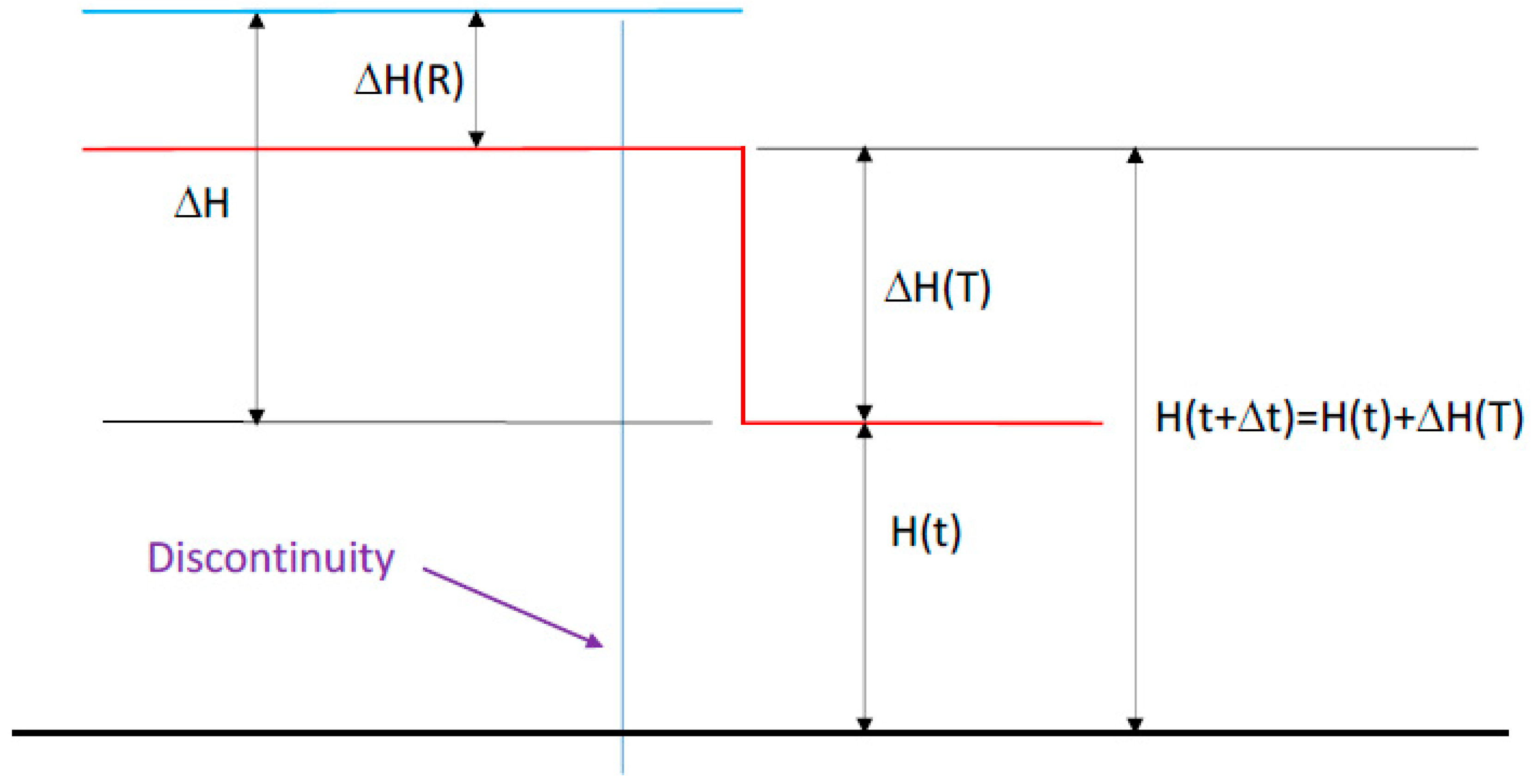
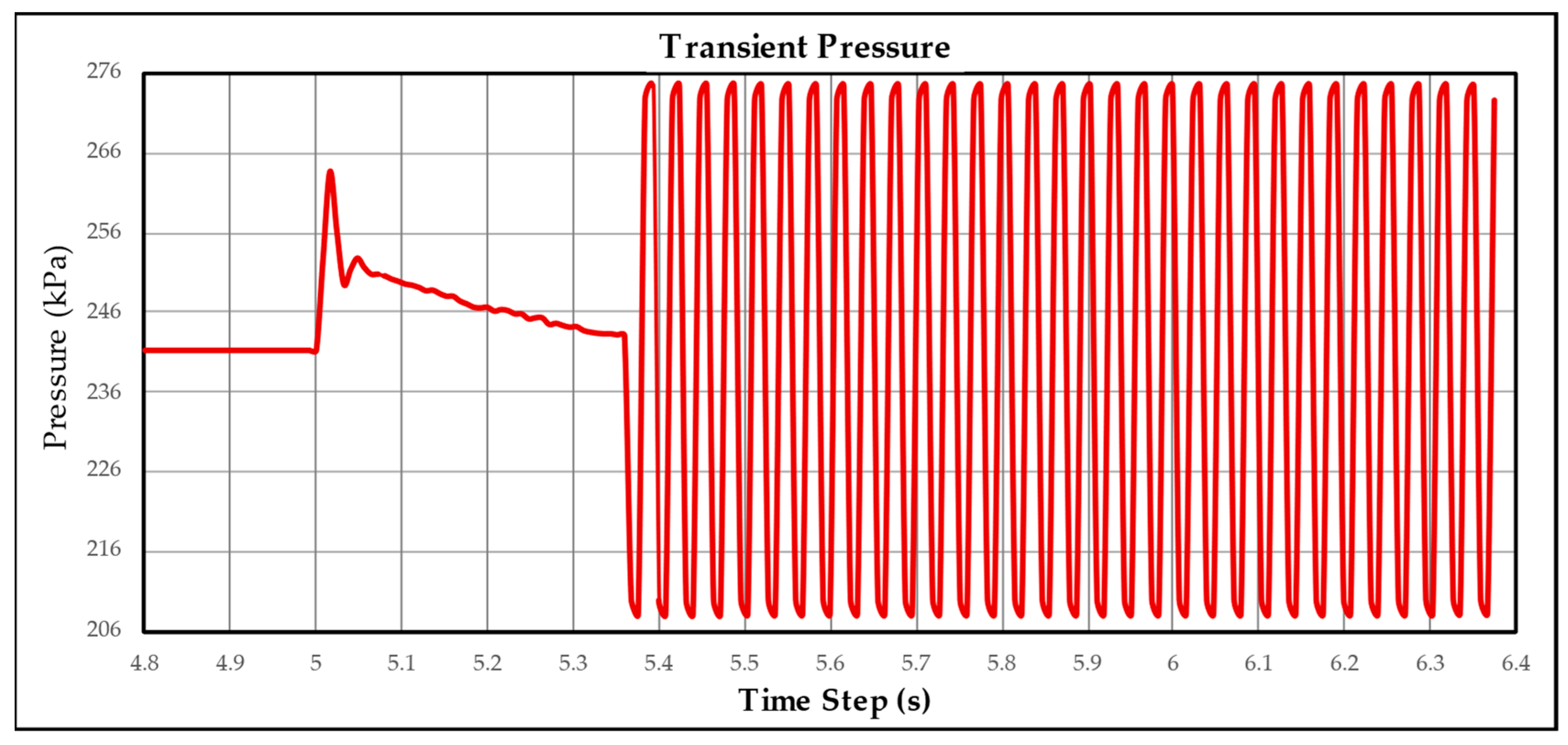
2.1. Transient Pressure and the Wave Plan Method
2.2. Effects and Consequences
2.3. Mitigation Strategies
2.4. Literature Review on Sonification
3. Methodology
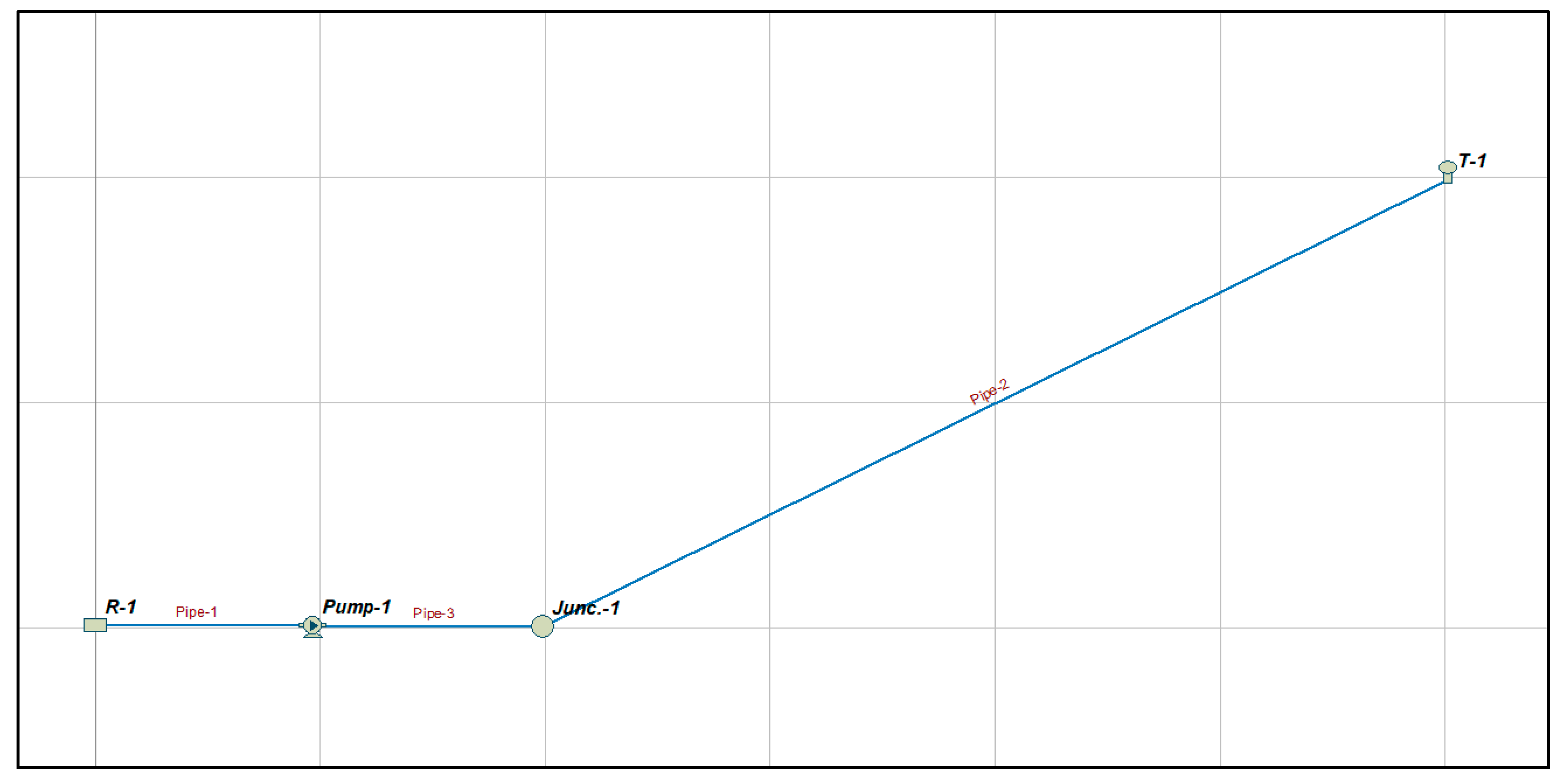
3.1. Hydraulic Model
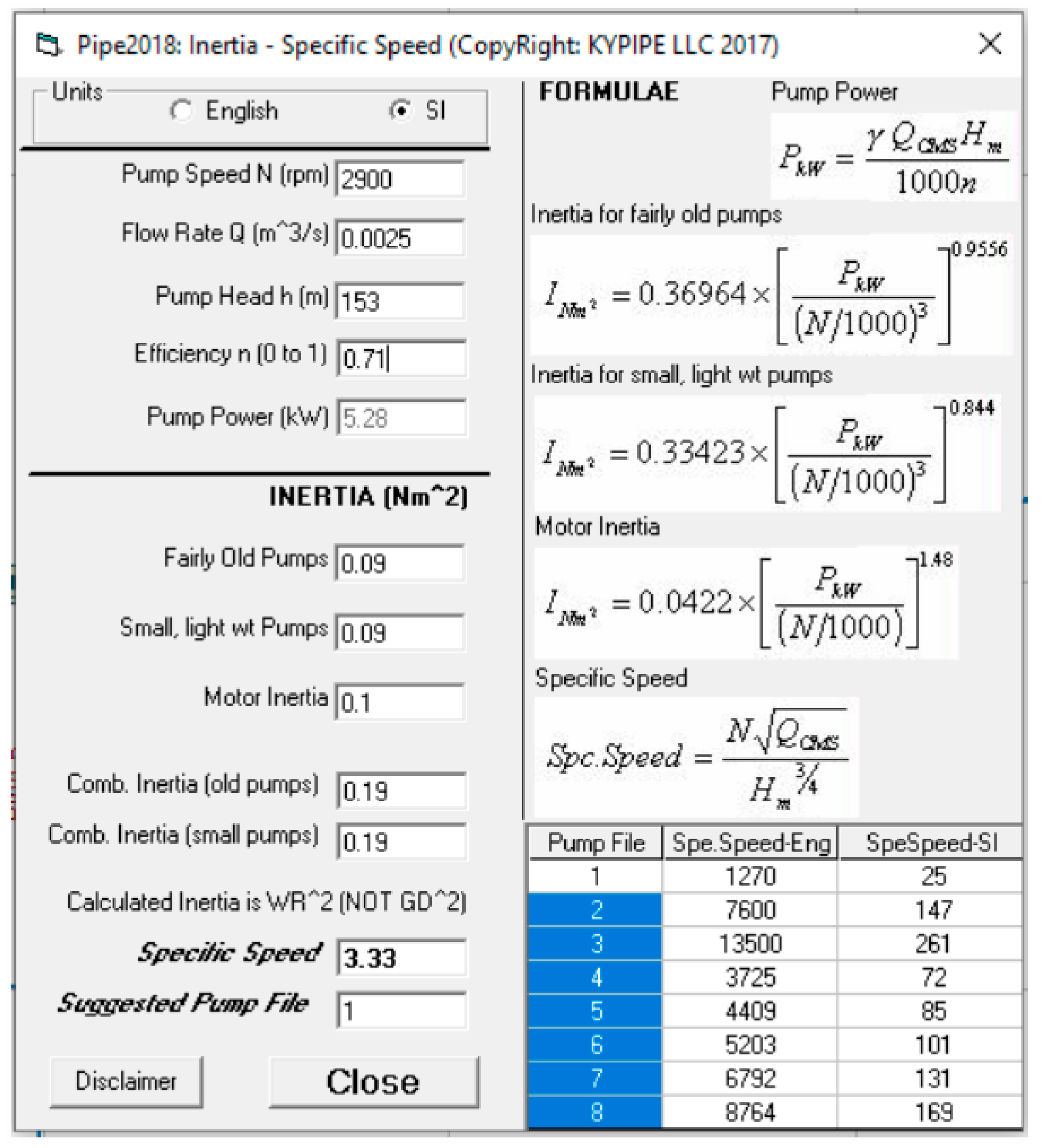
3.2. Pump File Number and Inertia
3.3. The Major Scale
3.4. Sound Mapping and Sound Library
4. Results
5. Limitation and Practical Considerations
6. Conclusions and Recommendations
Funding
Data Availability Statement
Conflicts of Interest
Appendix A
Appendix A.1. VBA CODE
| Sub Play_Data_Freq() Dim rng_Data As Range Dim i As Integer, iRow As Integer, iFreq As Integer Dim sFolderPath As String, sAudioFile As String Set rng_Data = Sh_Data.Range(“B2”, Range(“B2”).End(xlDown).Address) ‘Change the path below for the music library sFolderPath = “C:\Users\Khizer\Documents\UdaytonNew\Independent Study\SoundLibrary” ‘Traverse rows in the data sheet For i = 1 To rng_Data.Rows.Count iFreq = rng_Data.Cells(i, 1) On Error Resume Next ‘Lookup the filename in Frequency sheet for the data and get the closest (same or next biggest) match iRow = WorksheetFunction.Match(Round(iFreq, 0), Sh_Freq.Range(“A:A”), 2) If iRow > 0 Then rng_Data.Cells(i, 1).Offset(0, 1) = Sh_Freq.Range(“B” & iRow) ‘Play the file in Syncronous mode ‘The filename is derived based on frequency vs Filename data in the Frequency sheet SoundMe (sFolderPath & “\” & Sh_Freq.Range(“B” & iRow) & “.wav”) End If Next i End Sub |
Appendix A.2. KYPipe Simulation Results

| Time Step (s) | Pressure (kPa) | Time Step (s) | Pressure (kPa) |
|---|---|---|---|
| 0 | 241.25 | 4.992 | 241.25 |
| 0.008 | 241.25 | 5 | 241.25 |
| 0.016 | 241.25 | 5.008 | 252.83 |
| 0.024 | 241.25 | 5.016 | 263.59 |
| 0.032 | 241.25 | 5.024 | 256.14 |
| 0.04 | 241.25 | 5.032 | 249.52 |
| 0.048 | 241.25 | 5.04 | 251.31 |
| 0.056 | 241.25 | 5.048 | 252.76 |
| 0.064 | 241.25 | 5.056 | 251.59 |
| 0.072 | 241.25 | 5.064 | 250.76 |
| 0.08 | 241.25 | 5.072 | 250.76 |
| 0.088 | 241.25 | 5.08 | 250.56 |
| 0.096 | 241.25 | 5.088 | 250.14 |
| 0.104 | 241.25 | 5.096 | 249.87 |
| 0.112 | 241.25 | 5.104 | 249.52 |
| 0.12 | 241.25 | 5.112 | 249.38 |
| 0.128 | 241.25 | 5.12 | 249.11 |
| 0.136 | 241.25 | 5.128 | 248.69 |
| 0.144 | 241.25 | 5.136 | 248.76 |
| 0.152 | 241.25 | 5.144 | 248.35 |
| 0.16 | 241.25 | 5.152 | 248 |
| 0.168 | 241.25 | 5.16 | 248 |
| 0.176 | 241.25 | 5.168 | 247.38 |
| 0.184 | 241.25 | 5.176 | 247.04 |
| 0.192 | 241.25 | 5.184 | 246.63 |
| 0.2 | 241.25 | 5.192 | 246.56 |
| 0.208 | 241.25 | 5.2 | 246.63 |
| 0.216 | 241.25 | 5.208 | 246.14 |
| 0.224 | 241.25 | 5.216 | 246.35 |
| 0.232 | 241.25 | 5.224 | 246.21 |
| 0.24 | 241.25 | 5.232 | 245.8 |
| 0.248 | 241.25 | 5.24 | 245.8 |
| 0.256 | 241.25 | 5.248 | 245.18 |
| 0.264 | 241.25 | 5.256 | 245.32 |
| 0.272 | 241.25 | 5.264 | 245.32 |
| 0.28 | 241.25 | 5.272 | 244.49 |
| 0.288 | 241.25 | 5.28 | 244.63 |
| 0.296 | 241.25 | 5.288 | 244.35 |
| 0.304 | 241.25 | 5.296 | 244.14 |
| 0.312 | 241.25 | 5.304 | 244.21 |
| 0.32 | 241.25 | 5.312 | 243.73 |
| 0.328 | 241.25 | 5.32 | 243.52 |
| 0.336 | 241.25 | 5.328 | 243.39 |
| 0.344 | 241.25 | 5.336 | 243.32 |
| 0.352 | 241.25 | 5.344 | 243.32 |
| 0.36 | 241.25 | 5.352 | 243.18 |
| 0.368 | 241.25 | 5.36 | 243.11 |
| 0.376 | 241.25 | 5.368 | 210.01 |
| 0.384 | 241.25 | 5.376 | 208.29 |
| 0.392 | 241.25 | 5.384 | 272.62 |
| 0.4 | 241.25 | 5.392 | 274.34 |
| 0.408 | 241.25 | 5.4 | 210.01 |
| 0.416 | 241.25 | 5.408 | 208.29 |
| 0.424 | 241.25 | 5.416 | 272.62 |
| 0.432 | 241.25 | 5.424 | 274.34 |
| 0.44 | 241.25 | 5.432 | 210.01 |
| 0.448 | 241.25 | 5.44 | 208.29 |
| 0.456 | 241.25 | 5.448 | 272.62 |
| 0.464 | 241.25 | 5.456 | 274.34 |
| 0.472 | 241.25 | 5.464 | 210.08 |
| 0.48 | 241.25 | 5.472 | 208.29 |
| 0.488 | 241.25 | 5.48 | 272.55 |
| 0.496 | 241.25 | 5.488 | 274.34 |
| 0.504 | 241.25 | 5.496 | 210.08 |
| 0.512 | 241.25 | 5.504 | 208.36 |
| 0.52 | 241.25 | 5.512 | 272.55 |
| 0.528 | 241.25 | 5.52 | 274.27 |
| 0.536 | 241.25 | 5.528 | 210.08 |
| 0.544 | 241.25 | 5.536 | 208.36 |
| 0.552 | 241.25 | 5.544 | 272.55 |
| 0.56 | 241.25 | 5.552 | 274.27 |
| 0.568 | 241.25 | 5.56 | 210.08 |
| 0.576 | 241.25 | 5.568 | 208.36 |
| 0.584 | 241.25 | 5.576 | 272.55 |
| 0.592 | 241.25 | 5.584 | 274.27 |
| 0.6 | 241.25 | 5.592 | 210.08 |
| 0.608 | 241.25 | 5.6 | 208.36 |
| 0.616 | 241.25 | 5.608 | 272.55 |
| 0.624 | 241.25 | 5.616 | 274.27 |
| 0.632 | 241.25 | 5.624 | 210.08 |
| 0.64 | 241.25 | 5.632 | 208.36 |
| 0.648 | 241.25 | 5.64 | 272.55 |
| 0.656 | 241.25 | 5.648 | 274.27 |
| 0.664 | 241.25 | 5.656 | 210.08 |
| 0.672 | 241.25 | 5.664 | 208.36 |
| 0.68 | 241.25 | 5.672 | 272.55 |
| 0.688 | 241.25 | 5.68 | 274.27 |
| 0.696 | 241.25 | 5.688 | 210.08 |
| 0.704 | 241.25 | 5.696 | 208.36 |
| 0.712 | 241.25 | 5.704 | 272.55 |
| 0.72 | 241.25 | 5.712 | 274.27 |
| 0.728 | 241.25 | 5.72 | 210.08 |
| 0.736 | 241.25 | 5.728 | 208.36 |
| 0.744 | 241.25 | 5.736 | 272.55 |
| 0.752 | 241.25 | 5.744 | 274.27 |
| 0.76 | 241.25 | 5.752 | 210.08 |
| 0.768 | 241.25 | 5.76 | 208.36 |
| 0.776 | 241.25 | 5.768 | 272.55 |
| 0.784 | 241.25 | 5.776 | 274.27 |
| 0.792 | 241.25 | 5.784 | 210.08 |
| 0.8 | 241.25 | 5.792 | 208.36 |
| 0.808 | 241.25 | 5.8 | 272.55 |
| 0.816 | 241.25 | 5.808 | 274.27 |
| 0.824 | 241.25 | 5.816 | 210.08 |
| 0.832 | 241.25 | 5.824 | 208.36 |
| 0.84 | 241.25 | 5.832 | 272.55 |
| 0.848 | 241.25 | 5.84 | 274.27 |
| 0.856 | 241.25 | 5.848 | 210.08 |
| 0.864 | 241.25 | 5.856 | 208.36 |
| 0.872 | 241.25 | 5.864 | 272.55 |
| 0.88 | 241.25 | 5.872 | 274.27 |
| 0.888 | 241.25 | 5.88 | 210.08 |
| 0.896 | 241.25 | 5.888 | 208.36 |
| 0.904 | 241.25 | 5.896 | 272.55 |
| 0.912 | 241.25 | 5.904 | 274.27 |
| 0.92 | 241.25 | 5.912 | 210.08 |
| 0.928 | 241.25 | 5.92 | 208.36 |
| 0.936 | 241.25 | 5.928 | 272.55 |
| 0.944 | 241.25 | 5.936 | 274.27 |
| 0.952 | 241.25 | 5.944 | 210.08 |
| 0.96 | 241.25 | 5.952 | 208.36 |
| 0.968 | 241.25 | 5.96 | 272.55 |
| 0.976 | 241.25 | 5.968 | 274.27 |
| 0.984 | 241.25 | 5.976 | 210.08 |
| 0.992 | 241.25 | 5.984 | 208.36 |
| 1 | 241.25 | 5.992 | 272.55 |
| 1.008 | 241.25 | 6 | 274.27 |
| 1.016 | 241.25 | 6.008 | 210.08 |
| 1.024 | 241.25 | 6.016 | 208.36 |
| 1.032 | 241.25 | 6.024 | 272.55 |
| 1.04 | 241.25 | 6.032 | 274.27 |
| 1.048 | 241.25 | 6.04 | 210.08 |
| 1.056 | 241.25 | 6.048 | 208.36 |
| 1.064 | 241.25 | 6.056 | 272.55 |
| 1.072 | 241.25 | 6.064 | 274.27 |
| 1.08 | 241.25 | 6.072 | 210.08 |
| 1.088 | 241.25 | 6.08 | 208.36 |
| 1.096 | 241.25 | 6.088 | 272.55 |
| 1.104 | 241.25 | 6.096 | 274.27 |
| 1.112 | 241.25 | 6.104 | 210.08 |
| 1.12 | 241.25 | 6.112 | 208.36 |
| 1.128 | 241.25 | 6.12 | 272.55 |
| 1.136 | 241.25 | 6.128 | 274.27 |
| 1.144 | 241.25 | 6.136 | 210.08 |
| 1.152 | 241.25 | 6.144 | 208.36 |
| 1.16 | 241.25 | 6.152 | 272.55 |
| 1.168 | 241.25 | 6.16 | 274.27 |
| 1.176 | 241.25 | 6.168 | 210.08 |
| 1.184 | 241.25 | 6.176 | 208.36 |
| 1.192 | 241.25 | 6.184 | 272.55 |
| 1.2 | 241.25 | 6.192 | 274.27 |
| 1.208 | 241.25 | 6.2 | 210.08 |
| 1.216 | 241.25 | 6.208 | 208.36 |
| 1.224 | 241.25 | 6.216 | 272.55 |
| 1.232 | 241.25 | 6.224 | 274.27 |
| 1.24 | 241.25 | 6.232 | 210.08 |
| 1.248 | 241.25 | 6.24 | 208.36 |
| 1.256 | 241.25 | 6.248 | 272.55 |
| 1.264 | 241.25 | 6.256 | 274.27 |
| 1.272 | 241.25 | 6.264 | 210.08 |
| 1.28 | 241.25 | 6.272 | 208.36 |
| 1.288 | 241.25 | 6.28 | 272.55 |
| 1.296 | 241.25 | 6.288 | 274.27 |
| 1.304 | 241.25 | 6.296 | 210.15 |
| 1.312 | 241.25 | 6.304 | 208.36 |
| 1.32 | 241.25 | 6.312 | 272.48 |
| 1.328 | 241.25 | 6.32 | 274.27 |
| 1.336 | 241.25 | 6.328 | 210.15 |
| 1.344 | 241.25 | 6.336 | 208.43 |
| 1.352 | 241.25 | 6.344 | 272.48 |
| 1.36 | 241.25 | 6.352 | 274.2 |
| 1.368 | 241.25 | 6.36 | 210.15 |
| 1.376 | 241.25 | 6.368 | 208.43 |
| 1.384 | 241.25 | 6.376 | 272.48 |
| 1.392 | 241.25 | 6.384 | 274.2 |
| 1.4 | 241.25 | 6.392 | 210.15 |
| 1.408 | 241.25 | 6.4 | 208.43 |
| 1.416 | 241.25 | 6.408 | 272.48 |
| 1.424 | 241.25 | 6.416 | 274.2 |
| 1.432 | 241.25 | 6.424 | 210.15 |
| 1.44 | 241.25 | 6.432 | 208.43 |
| 1.448 | 241.25 | 6.44 | 272.48 |
| 1.456 | 241.25 | 6.448 | 274.2 |
| 1.464 | 241.25 | 6.456 | 210.15 |
| 1.472 | 241.25 | 6.464 | 208.43 |
| 1.48 | 241.25 | 6.472 | 272.48 |
| 1.488 | 241.25 | 6.48 | 274.2 |
| 1.496 | 241.25 | 6.488 | 210.15 |
| 1.504 | 241.25 | 6.496 | 208.43 |
| 1.512 | 241.25 | 6.504 | 272.48 |
| 1.52 | 241.25 | 6.512 | 274.2 |
| 1.528 | 241.25 | 6.52 | 210.15 |
| 1.536 | 241.25 | 6.528 | 208.43 |
| 1.544 | 241.25 | 6.536 | 272.48 |
| 1.552 | 241.25 | 6.544 | 274.2 |
| 1.56 | 241.25 | 6.552 | 210.15 |
| 1.568 | 241.25 | 6.56 | 208.43 |
| 1.576 | 241.25 | 6.568 | 272.48 |
| 1.584 | 241.25 | 6.576 | 274.2 |
| 1.592 | 241.25 | 6.584 | 210.15 |
| 1.6 | 241.25 | 6.592 | 208.43 |
| 1.608 | 241.25 | 6.6 | 272.48 |
| 1.616 | 241.25 | 6.608 | 274.2 |
| 1.624 | 241.18 | 6.616 | 210.15 |
| 1.632 | 241.25 | 6.624 | 208.43 |
| 1.64 | 241.25 | 6.632 | 272.48 |
| 1.648 | 241.25 | 6.64 | 274.2 |
| 1.656 | 241.25 | 6.648 | 210.15 |
| 1.664 | 241.25 | 6.656 | 208.43 |
| 1.672 | 241.25 | 6.664 | 272.48 |
| 1.68 | 241.25 | 6.672 | 274.2 |
| 1.688 | 241.25 | 6.68 | 210.15 |
| 1.696 | 241.25 | 6.688 | 208.43 |
| 1.704 | 241.25 | 6.696 | 272.48 |
| 1.712 | 241.25 | 6.704 | 274.2 |
| 1.72 | 241.25 | 6.712 | 210.15 |
| 1.728 | 241.25 | 6.72 | 208.43 |
| 1.736 | 241.25 | 6.728 | 272.48 |
| 1.744 | 241.25 | 6.736 | 274.2 |
| 1.752 | 241.25 | 6.744 | 210.15 |
| 1.76 | 241.25 | 6.752 | 208.43 |
| 1.768 | 241.25 | 6.76 | 272.48 |
| 1.776 | 241.25 | 6.768 | 274.2 |
| 1.784 | 241.25 | 6.776 | 210.15 |
| 1.792 | 241.25 | 6.784 | 208.43 |
| 1.8 | 241.25 | 6.792 | 272.48 |
| 1.808 | 241.25 | 6.8 | 274.2 |
| 1.816 | 241.25 | 6.808 | 210.15 |
| 1.824 | 241.25 | 6.816 | 208.43 |
| 1.832 | 241.25 | 6.824 | 272.48 |
| 1.84 | 241.25 | 6.832 | 274.2 |
| 1.848 | 241.25 | 6.84 | 210.15 |
| 1.856 | 241.25 | 6.848 | 208.43 |
| 1.864 | 241.25 | 6.856 | 272.48 |
| 1.872 | 241.25 | 6.864 | 274.2 |
| 1.88 | 241.25 | 6.872 | 210.15 |
| 1.888 | 241.25 | 6.88 | 208.43 |
| 1.896 | 241.25 | 6.888 | 272.48 |
| 1.904 | 241.25 | 6.896 | 274.2 |
| 1.912 | 241.25 | 6.904 | 210.15 |
| 1.92 | 241.25 | 6.912 | 208.43 |
| 1.928 | 241.25 | 6.92 | 272.48 |
| 1.936 | 241.25 | 6.928 | 274.2 |
| 1.944 | 241.25 | 6.936 | 210.15 |
| 1.952 | 241.25 | 6.944 | 208.43 |
| 1.96 | 241.25 | 6.952 | 272.48 |
| 1.968 | 241.25 | 6.96 | 274.2 |
| 1.976 | 241.25 | 6.968 | 210.15 |
| 1.984 | 241.25 | 6.976 | 208.43 |
| 1.992 | 241.25 | 6.984 | 272.48 |
| 2 | 241.25 | 6.992 | 274.2 |
| 2.008 | 241.25 | 7 | 210.15 |
| 2.016 | 241.25 | 7.008 | 208.43 |
| 2.024 | 241.25 | 7.016 | 272.48 |
| 2.032 | 241.25 | 7.024 | 274.2 |
| 2.04 | 241.25 | 7.032 | 210.15 |
| 2.048 | 241.25 | 7.04 | 208.43 |
| 2.056 | 241.25 | 7.048 | 272.48 |
| 2.064 | 241.25 | 7.056 | 274.2 |
| 2.072 | 241.25 | 7.064 | 210.15 |
| 2.08 | 241.25 | 7.072 | 208.43 |
| 2.088 | 241.25 | 7.08 | 272.48 |
| 2.096 | 241.25 | 7.088 | 274.2 |
| 2.104 | 241.25 | 7.096 | 210.15 |
| 2.112 | 241.25 | 7.104 | 208.43 |
| 2.12 | 241.25 | 7.112 | 272.48 |
| 2.128 | 241.25 | 7.12 | 274.2 |
| 2.136 | 241.25 | 7.128 | 210.22 |
| 2.144 | 241.25 | 7.136 | 208.43 |
| 2.152 | 241.25 | 7.144 | 272.41 |
| 2.16 | 241.25 | 7.152 | 274.14 |
| 2.168 | 241.25 | 7.16 | 210.22 |
| 2.176 | 241.25 | 7.168 | 208.5 |
| 2.184 | 241.25 | 7.176 | 272.41 |
| 2.192 | 241.25 | 7.184 | 274.14 |
| 2.2 | 241.25 | 7.192 | 210.22 |
| 2.208 | 241.25 | 7.2 | 208.5 |
| 2.216 | 241.25 | 7.208 | 272.41 |
| 2.224 | 241.25 | 7.216 | 274.14 |
| 2.232 | 241.25 | 7.224 | 210.22 |
| 2.24 | 241.25 | 7.232 | 208.5 |
| 2.248 | 241.25 | 7.24 | 272.41 |
| 2.256 | 241.25 | 7.248 | 274.14 |
| 2.264 | 241.25 | 7.256 | 210.22 |
| 2.272 | 241.25 | 7.264 | 208.5 |
| 2.28 | 241.25 | 7.272 | 272.41 |
| 2.288 | 241.25 | 7.28 | 274.14 |
| 2.296 | 241.25 | 7.288 | 210.22 |
| 2.304 | 241.25 | 7.296 | 208.5 |
| 2.312 | 241.25 | 7.304 | 272.41 |
| 2.32 | 241.25 | 7.312 | 274.14 |
| 2.328 | 241.25 | 7.32 | 210.22 |
| 2.336 | 241.25 | 7.328 | 208.5 |
| 2.344 | 241.25 | 7.336 | 272.41 |
| 2.352 | 241.25 | 7.344 | 274.14 |
| 2.36 | 241.25 | 7.352 | 210.22 |
| 2.368 | 241.25 | 7.36 | 208.5 |
| 2.376 | 241.25 | 7.368 | 272.41 |
| 2.384 | 241.25 | 7.376 | 274.14 |
| 2.392 | 241.25 | 7.384 | 210.22 |
| 2.4 | 241.25 | 7.392 | 208.5 |
| 2.408 | 241.25 | 7.4 | 272.41 |
| 2.416 | 241.25 | 7.408 | 274.14 |
| 2.424 | 241.25 | 7.416 | 210.22 |
| 2.432 | 241.25 | 7.424 | 208.5 |
| 2.44 | 241.25 | 7.432 | 272.41 |
| 2.448 | 241.25 | 7.44 | 274.14 |
| 2.456 | 241.25 | 7.448 | 210.22 |
| 2.464 | 241.25 | 7.456 | 208.5 |
| 2.472 | 241.25 | 7.464 | 272.41 |
| 2.48 | 241.25 | 7.472 | 274.14 |
| 2.488 | 241.25 | 7.48 | 210.22 |
| 2.496 | 241.25 | 7.488 | 208.5 |
| 2.504 | 241.25 | 7.496 | 272.41 |
| 2.512 | 241.25 | 7.504 | 274.14 |
| 2.52 | 241.25 | 7.512 | 210.22 |
| 2.528 | 241.25 | 7.52 | 208.5 |
| 2.536 | 241.25 | 7.528 | 272.41 |
| 2.544 | 241.25 | 7.536 | 274.14 |
| 2.552 | 241.25 | 7.544 | 210.22 |
| 2.56 | 241.25 | 7.552 | 208.5 |
| 2.568 | 241.25 | 7.56 | 272.41 |
| 2.576 | 241.25 | 7.568 | 274.14 |
| 2.584 | 241.25 | 7.576 | 210.22 |
| 2.592 | 241.25 | 7.584 | 208.5 |
| 2.6 | 241.25 | 7.592 | 272.41 |
| 2.608 | 241.25 | 7.6 | 274.14 |
| 2.616 | 241.25 | 7.608 | 210.22 |
| 2.624 | 241.25 | 7.616 | 208.5 |
| 2.632 | 241.25 | 7.624 | 272.41 |
| 2.64 | 241.25 | 7.632 | 274.14 |
| 2.648 | 241.25 | 7.64 | 210.22 |
| 2.656 | 241.25 | 7.648 | 208.5 |
| 2.664 | 241.25 | 7.656 | 272.41 |
| 2.672 | 241.25 | 7.664 | 274.14 |
| 2.68 | 241.25 | 7.672 | 210.22 |
| 2.688 | 241.25 | 7.68 | 208.5 |
| 2.696 | 241.25 | 7.688 | 272.41 |
| 2.704 | 241.25 | 7.696 | 274.14 |
| 2.712 | 241.25 | 7.704 | 210.22 |
| 2.72 | 241.25 | 7.712 | 208.5 |
| 2.728 | 241.25 | 7.72 | 272.41 |
| 2.736 | 241.25 | 7.728 | 274.14 |
| 2.744 | 241.25 | 7.736 | 210.22 |
| 2.752 | 241.25 | 7.744 | 208.5 |
| 2.76 | 241.25 | 7.752 | 272.41 |
| 2.768 | 241.25 | 7.76 | 274.14 |
| 2.776 | 241.25 | 7.768 | 210.22 |
| 2.784 | 241.25 | 7.776 | 208.5 |
| 2.792 | 241.25 | 7.784 | 272.41 |
| 2.8 | 241.25 | 7.792 | 274.14 |
| 2.808 | 241.25 | 7.8 | 210.22 |
| 2.816 | 241.25 | 7.808 | 208.5 |
| 2.824 | 241.25 | 7.816 | 272.41 |
| 2.832 | 241.25 | 7.824 | 274.14 |
| 2.84 | 241.25 | 7.832 | 210.22 |
| 2.848 | 241.25 | 7.84 | 208.5 |
| 2.856 | 241.25 | 7.848 | 272.41 |
| 2.864 | 241.25 | 7.856 | 274.14 |
| 2.872 | 241.25 | 7.864 | 210.22 |
| 2.88 | 241.25 | 7.872 | 208.5 |
| 2.888 | 241.25 | 7.88 | 272.41 |
| 2.896 | 241.25 | 7.888 | 274.14 |
| 2.904 | 241.25 | 7.896 | 210.22 |
| 2.912 | 241.25 | 7.904 | 208.5 |
| 2.92 | 241.25 | 7.912 | 272.41 |
| 2.928 | 241.25 | 7.92 | 274.14 |
| 2.936 | 241.25 | 7.928 | 210.22 |
| 2.944 | 241.25 | 7.936 | 208.5 |
| 2.952 | 241.25 | 7.944 | 272.41 |
| 2.96 | 241.25 | 7.952 | 274.14 |
| 2.968 | 241.25 | 7.96 | 210.22 |
| 2.976 | 241.25 | 7.968 | 208.57 |
| 2.984 | 241.25 | 7.976 | 272.41 |
| 2.992 | 241.25 | 7.984 | 274.07 |
| 3 | 241.25 | 7.992 | 210.29 |
| 3.008 | 241.25 | 8 | 208.57 |
| 3.016 | 241.25 | 8.008 | 272.34 |
| 3.024 | 241.25 | 8.016 | 274.07 |
| 3.032 | 241.25 | 8.024 | 210.29 |
| 3.04 | 241.25 | 8.032 | 208.57 |
| 3.048 | 241.25 | 8.04 | 272.34 |
| 3.056 | 241.25 | 8.048 | 274.07 |
| 3.064 | 241.25 | 8.056 | 210.29 |
| 3.072 | 241.25 | 8.064 | 208.57 |
| 3.08 | 241.25 | 8.072 | 272.34 |
| 3.088 | 241.25 | 8.08 | 274.07 |
| 3.096 | 241.25 | 8.088 | 210.29 |
| 3.104 | 241.25 | 8.096 | 208.57 |
| 3.112 | 241.25 | 8.104 | 272.34 |
| 3.12 | 241.25 | 8.112 | 274.07 |
| 3.128 | 241.25 | 8.12 | 210.29 |
| 3.136 | 241.25 | 8.128 | 208.57 |
| 3.144 | 241.25 | 8.136 | 272.34 |
| 3.152 | 241.25 | 8.144 | 274.07 |
| 3.16 | 241.25 | 8.152 | 210.29 |
| 3.168 | 241.25 | 8.16 | 208.57 |
| 3.176 | 241.25 | 8.168 | 272.34 |
| 3.184 | 241.25 | 8.176 | 274.07 |
| 3.192 | 241.25 | 8.184 | 210.29 |
| 3.2 | 241.25 | 8.192 | 208.57 |
| 3.208 | 241.25 | 8.2 | 272.34 |
| 3.216 | 241.25 | 8.208 | 274.07 |
| 3.224 | 241.25 | 8.216 | 210.29 |
| 3.232 | 241.25 | 8.224 | 208.57 |
| 3.24 | 241.25 | 8.232 | 272.34 |
| 3.248 | 241.25 | 8.24 | 274.07 |
| 3.256 | 241.25 | 8.248 | 210.29 |
| 3.264 | 241.25 | 8.256 | 208.57 |
| 3.272 | 241.25 | 8.264 | 272.34 |
| 3.28 | 241.25 | 8.272 | 274.07 |
| 3.288 | 241.25 | 8.28 | 210.29 |
| 3.296 | 241.25 | 8.288 | 208.57 |
| 3.304 | 241.25 | 8.296 | 272.34 |
| 3.312 | 241.25 | 8.304 | 274.07 |
| 3.32 | 241.25 | 8.312 | 210.29 |
| 3.328 | 241.25 | 8.32 | 208.57 |
| 3.336 | 241.25 | 8.328 | 272.34 |
| 3.344 | 241.25 | 8.336 | 274.07 |
| 3.352 | 241.25 | 8.344 | 210.29 |
| 3.36 | 241.25 | 8.352 | 208.57 |
| 3.368 | 241.25 | 8.36 | 272.34 |
| 3.376 | 241.25 | 8.368 | 274.07 |
| 3.384 | 241.25 | 8.376 | 210.29 |
| 3.392 | 241.25 | 8.384 | 208.57 |
| 3.4 | 241.25 | 8.392 | 272.34 |
| 3.408 | 241.25 | 8.4 | 274.07 |
| 3.416 | 241.25 | 8.408 | 210.29 |
| 3.424 | 241.25 | 8.416 | 208.57 |
| 3.432 | 241.25 | 8.424 | 272.34 |
| 3.44 | 241.25 | 8.432 | 274.07 |
| 3.448 | 241.25 | 8.44 | 210.29 |
| 3.456 | 241.25 | 8.448 | 208.57 |
| 3.464 | 241.25 | 8.456 | 272.34 |
| 3.472 | 241.25 | 8.464 | 274.07 |
| 3.48 | 241.25 | 8.472 | 210.29 |
| 3.488 | 241.25 | 8.48 | 208.57 |
| 3.496 | 241.25 | 8.488 | 272.34 |
| 3.504 | 241.25 | 8.496 | 274.07 |
| 3.512 | 241.25 | 8.504 | 210.29 |
| 3.52 | 241.25 | 8.512 | 208.57 |
| 3.528 | 241.25 | 8.52 | 272.34 |
| 3.536 | 241.25 | 8.528 | 274.07 |
| 3.544 | 241.25 | 8.536 | 210.29 |
| 3.552 | 241.25 | 8.544 | 208.57 |
| 3.56 | 241.25 | 8.552 | 272.34 |
| 3.568 | 241.25 | 8.56 | 274.07 |
| 3.576 | 241.25 | 8.568 | 210.29 |
| 3.584 | 241.25 | 8.576 | 208.57 |
| 3.592 | 241.25 | 8.584 | 272.34 |
| 3.6 | 241.25 | 8.592 | 274.07 |
| 3.608 | 241.25 | 8.6 | 210.29 |
| 3.616 | 241.25 | 8.608 | 208.57 |
| 3.624 | 241.25 | 8.616 | 272.34 |
| 3.632 | 241.25 | 8.624 | 274.07 |
| 3.64 | 241.25 | 8.632 | 210.29 |
| 3.648 | 241.25 | 8.64 | 208.57 |
| 3.656 | 241.25 | 8.648 | 272.34 |
| 3.664 | 241.25 | 8.656 | 274.07 |
| 3.672 | 241.25 | 8.664 | 210.29 |
| 3.68 | 241.25 | 8.672 | 208.57 |
| 3.688 | 241.25 | 8.68 | 272.34 |
| 3.696 | 241.25 | 8.688 | 274.07 |
| 3.704 | 241.25 | 8.696 | 210.29 |
| 3.712 | 241.25 | 8.704 | 208.57 |
| 3.72 | 241.25 | 8.712 | 272.34 |
| 3.728 | 241.25 | 8.72 | 274.07 |
| 3.736 | 241.25 | 8.728 | 210.29 |
| 3.744 | 241.25 | 8.736 | 208.57 |
| 3.752 | 241.25 | 8.744 | 272.34 |
| 3.76 | 241.25 | 8.752 | 274.07 |
| 3.768 | 241.25 | 8.76 | 210.29 |
| 3.776 | 241.25 | 8.768 | 208.57 |
| 3.784 | 241.25 | 8.776 | 272.34 |
| 3.792 | 241.25 | 8.784 | 274.07 |
| 3.8 | 241.25 | 8.792 | 210.29 |
| 3.808 | 241.25 | 8.8 | 208.64 |
| 3.816 | 241.25 | 8.808 | 272.34 |
| 3.824 | 241.25 | 8.816 | 274 |
| 3.832 | 241.25 | 8.824 | 210.29 |
| 3.84 | 241.25 | 8.832 | 208.64 |
| 3.848 | 241.25 | 8.84 | 272.27 |
| 3.856 | 241.25 | 8.848 | 274 |
| 3.864 | 241.25 | 8.856 | 210.36 |
| 3.872 | 241.25 | 8.864 | 208.64 |
| 3.88 | 241.25 | 8.872 | 272.27 |
| 3.888 | 241.25 | 8.88 | 274 |
| 3.896 | 241.25 | 8.888 | 210.36 |
| 3.904 | 241.25 | 8.896 | 208.64 |
| 3.912 | 241.25 | 8.904 | 272.27 |
| 3.92 | 241.25 | 8.912 | 274 |
| 3.928 | 241.25 | 8.92 | 210.36 |
| 3.936 | 241.25 | 8.928 | 208.64 |
| 3.944 | 241.25 | 8.936 | 272.27 |
| 3.952 | 241.25 | 8.944 | 274 |
| 3.96 | 241.25 | 8.952 | 210.36 |
| 3.968 | 241.25 | 8.96 | 208.64 |
| 3.976 | 241.25 | 8.968 | 272.27 |
| 3.984 | 241.25 | 8.976 | 274 |
| 3.992 | 241.25 | 8.984 | 210.36 |
| 4 | 241.25 | 8.992 | 208.64 |
| 4.008 | 241.25 | 9 | 272.27 |
| 4.016 | 241.25 | 9.008 | 274 |
| 4.024 | 241.25 | 9.016 | 210.36 |
| 4.032 | 241.25 | 9.024 | 208.64 |
| 4.04 | 241.25 | 9.032 | 272.27 |
| 4.048 | 241.25 | 9.04 | 274 |
| 4.056 | 241.25 | 9.048 | 210.36 |
| 4.064 | 241.25 | 9.056 | 208.64 |
| 4.072 | 241.25 | 9.064 | 272.27 |
| 4.08 | 241.25 | 9.072 | 274 |
| 4.088 | 241.25 | 9.08 | 210.36 |
| 4.096 | 241.25 | 9.088 | 208.64 |
| 4.104 | 241.25 | 9.096 | 272.27 |
| 4.112 | 241.25 | 9.104 | 274 |
| 4.12 | 241.25 | 9.112 | 210.36 |
| 4.128 | 241.25 | 9.12 | 208.64 |
| 4.136 | 241.25 | 9.128 | 272.27 |
| 4.144 | 241.25 | 9.136 | 274 |
| 4.152 | 241.25 | 9.144 | 210.36 |
| 4.16 | 241.25 | 9.152 | 208.64 |
| 4.168 | 241.25 | 9.16 | 272.27 |
| 4.176 | 241.25 | 9.168 | 274 |
| 4.184 | 241.25 | 9.176 | 210.36 |
| 4.192 | 241.25 | 9.184 | 208.64 |
| 4.2 | 241.25 | 9.192 | 272.27 |
| 4.208 | 241.25 | 9.2 | 274 |
| 4.216 | 241.25 | 9.208 | 210.36 |
| 4.224 | 241.25 | 9.216 | 208.64 |
| 4.232 | 241.25 | 9.224 | 272.27 |
| 4.24 | 241.25 | 9.232 | 274 |
| 4.248 | 241.25 | 9.24 | 210.36 |
| 4.256 | 241.25 | 9.248 | 208.64 |
| 4.264 | 241.25 | 9.256 | 272.27 |
| 4.272 | 241.25 | 9.264 | 274 |
| 4.28 | 241.25 | 9.272 | 210.36 |
| 4.288 | 241.25 | 9.28 | 208.64 |
| 4.296 | 241.25 | 9.288 | 272.27 |
| 4.304 | 241.25 | 9.296 | 274 |
| 4.312 | 241.25 | 9.304 | 210.36 |
| 4.32 | 241.25 | 9.312 | 208.64 |
| 4.328 | 241.25 | 9.32 | 272.27 |
| 4.336 | 241.25 | 9.328 | 274 |
| 4.344 | 241.25 | 9.336 | 210.36 |
| 4.352 | 241.25 | 9.344 | 208.64 |
| 4.36 | 241.25 | 9.352 | 272.27 |
| 4.368 | 241.25 | 9.36 | 274 |
| 4.376 | 241.25 | 9.368 | 210.36 |
| 4.384 | 241.25 | 9.376 | 208.64 |
| 4.392 | 241.25 | 9.384 | 272.27 |
| 4.4 | 241.25 | 9.392 | 274 |
| 4.408 | 241.25 | 9.4 | 210.36 |
| 4.416 | 241.25 | 9.408 | 208.64 |
| 4.424 | 241.25 | 9.416 | 272.27 |
| 4.432 | 241.25 | 9.424 | 274 |
| 4.44 | 241.25 | 9.432 | 210.36 |
| 4.448 | 241.25 | 9.44 | 208.64 |
| 4.456 | 241.25 | 9.448 | 272.27 |
| 4.464 | 241.25 | 9.456 | 274 |
| 4.472 | 241.25 | 9.464 | 210.36 |
| 4.48 | 241.25 | 9.472 | 208.64 |
| 4.488 | 241.25 | 9.48 | 272.27 |
| 4.496 | 241.25 | 9.488 | 274 |
| 4.504 | 241.25 | 9.496 | 210.36 |
| 4.512 | 241.25 | 9.504 | 208.64 |
| 4.52 | 241.25 | 9.512 | 272.27 |
| 4.528 | 241.25 | 9.52 | 274 |
| 4.536 | 241.25 | 9.528 | 210.36 |
| 4.544 | 241.25 | 9.536 | 208.64 |
| 4.552 | 241.25 | 9.544 | 272.27 |
| 4.56 | 241.25 | 9.552 | 274 |
| 4.568 | 241.25 | 9.56 | 210.36 |
| 4.576 | 241.25 | 9.568 | 208.64 |
| 4.584 | 241.25 | 9.576 | 272.27 |
| 4.592 | 241.25 | 9.584 | 274 |
| 4.6 | 241.25 | 9.592 | 210.36 |
| 4.608 | 241.25 | 9.6 | 208.64 |
| 4.616 | 241.25 | 9.608 | 272.27 |
| 4.624 | 241.25 | 9.616 | 274 |
| 4.632 | 241.25 | 9.624 | 210.36 |
| 4.64 | 241.25 | 9.632 | 208.64 |
| 4.648 | 241.25 | 9.64 | 272.27 |
| 4.656 | 241.25 | 9.648 | 273.93 |
| 4.664 | 241.25 | 9.656 | 210.36 |
| 4.672 | 241.25 | 9.664 | 208.7 |
| 4.68 | 241.25 | 9.672 | 272.27 |
| 4.688 | 241.25 | 9.68 | 273.93 |
| 4.696 | 241.25 | 9.688 | 210.43 |
| 4.704 | 241.25 | 9.696 | 208.7 |
| 4.712 | 241.25 | 9.704 | 272.21 |
| 4.72 | 241.25 | 9.712 | 273.93 |
| 4.728 | 241.25 | 9.72 | 210.43 |
| 4.736 | 241.25 | 9.728 | 208.7 |
| 4.744 | 241.25 | 9.736 | 272.21 |
| 4.752 | 241.25 | 9.744 | 273.93 |
| 4.76 | 241.25 | 9.752 | 210.43 |
| 4.768 | 241.25 | 9.76 | 208.7 |
| 4.776 | 241.25 | 9.768 | 272.21 |
| 4.784 | 241.25 | 9.776 | 273.93 |
| 4.792 | 241.25 | 9.784 | 210.43 |
| 4.8 | 241.25 | 9.792 | 208.7 |
| 4.808 | 241.25 | 9.8 | 272.21 |
| 4.816 | 241.25 | 9.808 | 273.93 |
| 4.824 | 241.25 | 9.816 | 210.43 |
| 4.832 | 241.25 | 9.824 | 208.7 |
| 4.84 | 241.25 | 9.832 | 272.21 |
| 4.848 | 241.25 | 9.84 | 273.93 |
| 4.856 | 241.25 | 9.848 | 210.43 |
| 4.864 | 241.25 | 9.856 | 208.7 |
| 4.872 | 241.25 | 9.864 | 272.21 |
| 4.88 | 241.25 | 9.872 | 273.93 |
| 4.888 | 241.25 | 9.88 | 210.43 |
| 4.896 | 241.25 | 9.888 | 208.7 |
| 4.904 | 241.25 | 9.896 | 272.21 |
| 4.912 | 241.25 | 9.904 | 273.93 |
| 4.92 | 241.25 | 9.912 | 210.43 |
| 4.928 | 241.25 | 9.92 | 208.7 |
| 4.936 | 241.25 | 9.928 | 272.21 |
| 4.944 | 241.25 | 9.936 | 273.93 |
| 4.952 | 241.25 | 9.944 | 210.43 |
| 4.96 | 241.25 | 9.952 | 208.7 |
| 4.968 | 241.25 | 9.96 | 272.21 |
| 4.976 | 241.25 | 9.968 | 273.93 |
| 4.984 | 241.25 | 9.976 | 210.43 |
| 9.984 | 208.7 | ||
| 9.992 | 272.21 | ||
| 10 | 273.93 |
References
- Weiss, P.; Taruskin, R. Music in the Western World; Cengage Learning: Farmington Hills, MI, USA, 2007. [Google Scholar]
- Chase, D. Transient Analysis in Hydraulic Networks; University of Dayton: Dayton, OH, USA, 2020. [Google Scholar]
- Chaudhry, M.H. Applied Hydraulic Transients, 3rd ed.; Springer: Berlin/Heidelberg, Germany, 2014. [Google Scholar]
- Wylie, E.B.; Streeter, V.L. Fluid Transients in Systems; Prentice Hall: Englewood Cliffs, NJ, USA, 1993. [Google Scholar]
- Thorley, A.R.D. Fluid Transients in Pipeline Systems, 2nd ed.; Professional Engineering Publishing: London, UK, 2004. [Google Scholar]
- Lingireddy, S.; Wood, D. Surge Analysis and the Wave Plan Method: A Powerful, Accurate, and Stable Method for Water Hammer Studies; KYPipe: Cary, NC, USA, 2021. [Google Scholar]
- Wood, D.J.; Funk, J.E. Hydraulic transients in systems with significant pipe elasticity. J. Basic Eng. 1966, 88, 185–196. [Google Scholar]
- Tullis, J.P. Hydraulics of Pipelines: Pumps, Valves, Cavitation, Transients; John Wiley & Sons: Hoboken, NJ, USA, 1989. [Google Scholar]
- Bly, S. Presenting Information in Sound. In Proceedings of the 1982 Conference on Human Factors in Computing Systems, Gaithersburg, MD, USA, 15–17 March 1982. [Google Scholar]
- Zhao, H.; Plaisant, C.; Shneiderman, B.; Lazar, J. Data Sonification for Users with Visual Impairment. ACM Trans. Comput.-Hum. Interact. 2008, 15, 4. [Google Scholar] [CrossRef]
- Forssén, J.; Kaczmarek, T.; Alvarsson, J.; Lundén, P.; Nilsson, M.E. Auralization of traffic noise within the LISTEN project—Preliminary results for passenger car pass-by. In Proceedings of Euronoise 2009: Action on Noise in Europe; Kang, J., Ed.; Institute of Acoustics: Milton Keynes, UK, 2009; pp. 1–11. [Google Scholar]
- Lenzi, S.; Terenghi, G.; Taormina, R.; Galelli, S.; Ciuccarelli, P. Disclosing Cyber Attacks on Water Distribution Systems. An Experimental Approach to the Sonification of Threats and Anomalous Data. In Proceedings of the 25th International Conference on Auditory Display (ICAD 2019), Newcastle upon Tyne, UK, 23–27 June 2019. [Google Scholar]
- Axon, L.; Creese, S.; Goldsmith, M.; Nurse, J.R.C. Reflecting on the Use of Sonification for Network Monitoring. In ThinkMind; IARIA: Wilmington, DE, USA, 2016; pp. 254–261. [Google Scholar]
- Muralidharan, L.; Ali, S.; Alfieri, F.; Jorgensen, J.; Agrawal, M. Sonify: Making Visual Graphs Accessible. In Proceedings of the 1st International Conference on Human Interaction and Emerging Technologies (IHIET 2019), Nice, France, 22–24 August 2019. [Google Scholar]
- Wood, D.J.; Lingireddy, S.; Boulos, P.F. Numerical Methods for Modeling Transient Flow in Distribution Systems; MWH Soft Press: Broomfield, CO, USA, 2005. [Google Scholar]
- Suits, B.H. Physics of Music—Notes. Retrieved from Michigan Technological University. 2023. Available online: https://web.archive.org/web/20230129030505/https://pages.mtu.edu/~suits/Physicsofmusic.html (accessed on 10 January 2023).
- Hermann von Helmholtz, A.J. On the Sensations of Tone as a Physiological Basis for the Theory of Music; Green Longmans: London, UK, 1885. [Google Scholar]
- Zaman, K. Sonification of Transient Pressure (Water Hammer) in a Hydraulic Network [Video]. YouTube. Available online: https://www.youtube.com/watch?v=HYqgvy5XawI (accessed on 26 April 2023).
- Muggleton, J.M.; Yan, J.; Brennan, M.J. Pipeline leak detection using acoustic methods. J. Pipeline Syst. Eng. Pract. 2011, 2, 145–153. [Google Scholar]
- Zhou, C.; Zhang, Y.; Zhao, X. Machine learning-based anomaly detection for pipeline acoustic monitoring. Sensors 2020, 20, 724. [Google Scholar]
- Meniconi, S.; Brunone, B.; Ferrante, M. Water pipeline integrity assessment by means of unsteady-state tests. J. Hydraul. Eng. 2012, 138, 715–725. [Google Scholar]

| Pressure (kPa) | Musical Note | Pressure (kPa) | Musical Note |
|---|---|---|---|
| 206.84 | C0 | 245.51 | C4 |
| 208.35 | D0 | 246.89 | D4 |
| 209.79 | E0 | 248.21 | E4 |
| 211.22 | F0 | 249.59 | F4 |
| 212.36 | G0 | 250.97 | G4 |
| 213.74 | A0 | 252.35 | A4 |
| 215.12 | B0 | 253.73 | B4 |
| 216.50 | C1 | 255.11 | C5 |
| 217.87 | D1 | 256.47 | D5 |
| 219.25 | E1 | 257.86 | E5 |
| 220.63 | F1 | 259.24 | F5 |
| 222.01 | G1 | 260.62 | G5 |
| 223.39 | A1 | 261.99 | A5 |
| 224.77 | B1 | 263.37 | B5 |
| 226.15 | C2 | 264.75 | C6 |
| 227.53 | D2 | 266.13 | D6 |
| 228.91 | E2 | 267.51 | E6 |
| 230.28 | F2 | 268.91 | F6 |
| 231.66 | G2 | 270.28 | G6 |
| 233.04 | A2 | 271.66 | A6 |
| 234.42 | B2 | 273.04 | B6 |
| 235.80 | C3 | 274.42 | C7 |
| 237.18 | D3 | 275.79 | D7 |
| 238.56 | E3 | 277.17 | E7 |
| 239.94 | F3 | 278.55 | F7 |
| 241.32 | G3 | 279.93 | G7 |
| 242.70 | A3 | 281.31 | A7 |
| 244.07 | B3 | 282.69 | B7 |
Disclaimer/Publisher’s Note: The statements, opinions and data contained in all publications are solely those of the individual author(s) and contributor(s) and not of MDPI and/or the editor(s). MDPI and/or the editor(s) disclaim responsibility for any injury to people or property resulting from any ideas, methods, instructions or products referred to in the content. |
© 2025 by the author. Licensee MDPI, Basel, Switzerland. This article is an open access article distributed under the terms and conditions of the Creative Commons Attribution (CC BY) license (https://creativecommons.org/licenses/by/4.0/).
Share and Cite
Zaman, M.K. Auditory Representation of Transient Hydraulic Phenomena: A Novel Approach to Sonification of Pressure Waves in Hydraulic Systems. Water 2025, 17, 1950. https://doi.org/10.3390/w17131950
Zaman MK. Auditory Representation of Transient Hydraulic Phenomena: A Novel Approach to Sonification of Pressure Waves in Hydraulic Systems. Water. 2025; 17(13):1950. https://doi.org/10.3390/w17131950
Chicago/Turabian StyleZaman, Muhammad Khizer. 2025. "Auditory Representation of Transient Hydraulic Phenomena: A Novel Approach to Sonification of Pressure Waves in Hydraulic Systems" Water 17, no. 13: 1950. https://doi.org/10.3390/w17131950
APA StyleZaman, M. K. (2025). Auditory Representation of Transient Hydraulic Phenomena: A Novel Approach to Sonification of Pressure Waves in Hydraulic Systems. Water, 17(13), 1950. https://doi.org/10.3390/w17131950