Stability Analysis of Recent Failed Red Clay Landslides Influenced by Cracks and Rainfall Based on the XGBoost–PSO–SVR Model

Abstract

Currently, most studies on slope stability either neglect or consider only one of the two critical factors—rainfall conditions and crack state—that influence the stability of recent landslides. To address this limitation, eleven parameters, including slope height, internal friction angle, cohesion, rainfall conditions, and crack state, were selected as evaluation indexes. GeoStudio software 2018 R2 was also used to simulate the slope safety factor under various parameters, and 363 datasets were obtained. The eXtreme Gradient Boosting–Particle Swarm Optimization–Support Vector Regression (XGBoost–PSO–SVR) model was employed to train the simulation results and construct a predictive model. The MSE of XGBoost–PSO–SVR when compared with the MSE of the single-machine methods of XGBoost and PSO–SVR is reduced by 71.9% and 57.8%, respectively. Furthermore, when compared with four single-machine models—Decision Tree (DT), Naive Bayes (NB), Random Forest (RF), and K-Nearest Neighbors (KNN)—the XGBoost–PSO–SVR model had the smallest MSE of 0.0016 and the largest R² of 0.9919. Thus, the XGBoost–PSO–SVR model demonstrated superior training performance. The predicted safety factor for a recent landslide in Yongchun County, Fujian Province, China, during 4–7 November 2016 was 0.9658, which closely aligned with the actual conditions. This study could provide a new method for the stability prediction of recent landslides based on various factors, such as rainfall conditions and crack state.

1. Introduction

Among various geological disasters, landslides are characterized by their wide distribution, high frequency of occurrence, and significant damage. They can be divided into three categories according to the time that they occurred, i.e., ancient landslides, old landslides, and recent landslides. Ancient landslides refer to landslides that took place prior to the Holocene and are of higher stability. Old landslides refer to landslides that occurred during the Holocene and are currently stable overall but may be unstable locally. Recent landslides refer to landslides that just took place or are taking place and whose stability is poor; thus, this is the category that deserves the most attention in engineering. For recent landslides, a number of cracks are typically observed at their trailing edges, sides, and leading edges. These cracks often serve as ideal pathways for rainfall infiltration, which can significantly increase the risk of landslide recurrence, posing a threat to the safety of the people involved in the landslide disaster rescue on site. This issue is particularly prominent in red clay landslides, attributed to the inherent structure of red clay, which includes a high proportion of voids and fissures. As a result, this study mainly focuses on the stability analysis of recent red clay landslides considering the influence of cracks and rainfall.

Extensive research has been conducted on slope stability analysis, yielding substantial results. However, most studies focus on slopes before sliding occurs. Even though a few investigators have explored the stability of already failed slopes, their studies primarily focus on ancient or old landslides. For example, Yang et al., Hu et al., Zhu et al. and Frink et al. studied the stability of ancient or old landslides with field survey and monitoring, satellite remote sensing, optical remote sensing dynamic monitoring, drone aerial survey, and numerical simulation [1,2,3,4,5,6,7,8]. While these studies have contributed to understanding the resurrection of ancient or old landslides, the restoration of the shear strength of the slip zone in a recent landslide is limited, and surface cracks remain unblocked. Consequently, findings from ancient or old landslide studies cannot be directly applied to recent landslides. The stability of a recent landslide, i.e., the Gaokanzi Landslide in Xintang, Enshi, Hubei, China, was analyzed using the transfer coefficient method [9]. However, only the natural unit weight of the soil and the unit weight under a once-in-50-years heavy rain scenario were considered. The parameters such as the angle of internal friction and the cohesion of both the slide mass and the slide zone in the two scenarios were considered without considering the influence of cracks and rainfall infiltration. A hydraulic coupling numerical analysis was carried out to simulate the resurrection of a recent loess landslide by Wang et al. [10]. However, only three kinds of rainfall conditions, i.e., light rain, moderate rain, and heavy rainstorm, were considered, without considering the influence of crack state. The study by Wang et al. [11] shows that abundant loose material sources and dominant joint (crack) structures could provide fundamental conditions for the resurrection of a recent landslide and the transition from a shallow slide to a deep slide. In their study, only natural conditions and heavy rainfall scenarios were considered, which were insufficient. Recently, the reverse analysis method and cloud model method have been employed to evaluate the stability of a recent landslide [12]. However, the degree of influence of the length, width, depth, and position of cracks on the stability of the recent landslide was not considered.

Based on the above facts, previous researchers seldom considered both rainfall conditions and crack states simultaneously, despite their interaction and mutual constraints [13,14,15,16,17,18]. At present, machine learning is being widely used as a prediction approach in various fields. Every machine learning model, such as Decision Tree (DT) [19], K-Nearest Neighbors (KNN) [20], Naive Bayes (NB) [21], Random Forest (RF) [22], eXtreme Gradient Boosting (XGBoost) [23], and Support Vector Regression (SVR) [24], has its advantages and disadvantages. For example, the XGBoost model has the advantages of nonlinear data processing, low computational cost, fast operation speed, and improved prevention of overfitting [25,26]. However, it has the disadvantage of sensitivity to outliers. The SVR model can effectively solve practical issues, such as small sample sizes, nonlinearity, high dimensionality, and local minima, demonstrating excellent generalization performance [27,28]. However, it has the shortcomings of slow training and difficult parameter selection. It was believed that combining multiple single-machine learning models can yield a prediction model with superior performance [29,30,31,32].

In view of the above facts, in this study, based on a recent red clay landslide, crack state (mainly including width and depth) and rainfall conditions were considered simultaneously, in addition to nine parameters, such as slope height, slope angle, and the cohesion and degree of internal friction of soil. The stability analyses of the landslide with different parameter values were conducted using the software GeoStudio. Subsequently, an adaptive weighted XGBoost–PSO–SVR hybrid model was trained with the simulation results to establish a prediction model. The validity of the model was validated by comparing its prediction results with those of single-machine-learning models like XGBoost, PSO–SVR, and DT. Finally, the reliability of the model was further verified by a case study of a recent red clay landslide in Yongchun County, Fujian Province, China. This study provided a new approach for the stability analysis of recent landslides under the comprehensive consideration of various factors, particularly rainfall conditions and crack status.

2. Materials and Methods

2.1. Acquisition of Research Data

To analyze the real-time stability of the recent red clay landslide mentioned above under rainfall conditions, a finite element model was established using the software GeoStudio for numerical simulation. The slope soil was assumed to be a single layer of red clay. Generally, there are numerous scattered cracks on the slide mass of a recent landslide. It is a huge task to plot all the cracks in an actual model. Therefore, in this study, the cracks were simplified into three main types: the main crack in the slip zone, the crack at the top of the slope, and the crack on the slope face. The length and width of cracks could be equivalently processed using Equations (1) and (2). The depth of the cracks was assumed to be half of the main crack depth.

$$L_e={\displaystyle \frac{{\displaystyle \sum _{i=1}^n{l}_i{x}_i}}{{\displaystyle \sum _{i=1}^n{x}_i}}}$$

(1)

$$W_e={\displaystyle \frac{{\displaystyle \sum _{i=1}^n{\mathrm{w}}_i{x}_i}}{{\displaystyle \sum _{i=1}^n{x}_i}}}$$

(2)

where L_e and W_e are the equivalent length and width of a crack, respectively; l_i and w_i are the length and width of each crack in the slip zone, respectively; x_i is the horizontal distance of each crack from the center of the slip zone.

For a recent landslide, there exists a slip zone caused by the landslide. Meanwhile, the slip zone of a single-layer homogeneous soil slope can be approximately assumed to be circular. However, whether the final slip surface passed through this slip zone was determined with the numerical simulation of the software GeoStudio, without forcing the slip surface to pass through the slip zone in this simulation. Taking a model with a slope height of 10 m and a slope angle of 45° as an example, the final model is shown in Figure 1. In this figure, L_b represents the red clay layer base; L_r represents the recent failed red clay layer; S_z represents the slip zone; C_m represents the main crack in the slip zone; C_t represents the crack at the top of the slope; C_s represents the crack on the surface of slope; and W.T. represents the water table. The constitutive model of this model was selected as the Mohr–Coulomb model. Since the rainfall intensity in this simulation was relatively high, for the good infiltration channel cracks and slip zone soil, the rainfall intensity was set as a flow boundary. However, for the red clay layer without cracks, the rainfall boundary condition was set as a pressure water head boundary. The pressure water head was set as 0.02 m. The seepage in this model was transient seepage, and the influence of groundwater was not considered. Therefore, the groundwater level was set as close to the bottom of the slope as possible, which is evident from the position of W.T. in Figure 1.

The parameters selected for simulation included slope height (H), slope angle (β), cohesion (c), internal friction angle (φ), unit weight (γ), rainfall intensity (I_r), rainfall duration (D_r), main crack width (W_c), main crack depth (D_c), crack area ratio at the top of the slope (R_t), and crack area ratio on the surface of slope (R_f). The values of R_t and R_f can be directly obtained from field surveys of the slope. The ratios are calculated by dividing the total area of cracks by the total area of the slope surface for both the top and face of the slope. Slope height and slope angle directly influence the gravitational forces acting on the slope. The steeper the slope angle and the greater the slope height, the higher the likelihood of slope instability. Cohesion and internal friction angle are inherent properties that resist shear failure. Higher cohesion and internal friction angle values enhance slope stability. Unit weight affects the total weight of the slope soil mass. Rainfall intensity and duration directly determine the extent of water infiltration into the slope, which may reduce the soil’s shear strength and increase pore water pressure. The characteristics of cracks in the slope (represented W_c, D_c, S_t, and S_f) provide preferential pathways for water infiltration. This may accelerate the reduction in shear strength and increase the risk of slope instability. The interaction of these factors has a combined effect on the stability of the slope. In general, slope angle, cohesion, and rainfall intensity are the main factors affecting slope stability. According to the Engineering Geology Manual of China [33], the minimum unit weight of red clay is 16.5 kN/m³, and the maximum unit weight is 18.5 kN/m³. The benchmark values for the three groups were selected as 17.0 kN/m³, 17.5 kN/m³, and 18.0 kN/m³ using the equal division method. The grouping benchmark values for internal friction angle and unit weight were selected in the same way. The meteorological department defines rainfall less than 10 mm in 24 h as light rain, between 10 mm and 25 mm as moderate rain, and between 25 mm and 50 mm as heavy rain. Therefore, 10 mm, 25 mm, and 50 mm were selected as the benchmark values for each group. For parameters such as slope height, slope angle, and rainfall duration, the benchmark values were selected based on the common classification standards used by researchers [10,11,12]. The values of R_t and R_f were determined based on the range of crack area ratios commonly observed in recent landslides. The final benchmark values for each group of parameters are shown in

Table 1. Numerical simulation grouping of each parameter.

Group	H/m	β/(°)	c/kPa	φ/(°)	γ/(kN·m−3)	Dr/d	Ir/(mm·d−1)	Wc/m	Dc/m	Rt/%	Rf/%
Ⅰ	5	22.5	79.5	17.25	17.0	1	10	0.05	1	5	5
Ⅱ	10	45	65	16.50	17.5	2	25	0.10	2	10	10
Ⅲ	15	67.5	50.5	15.75	18.0	3	50	0.15	3	15	15

. The safety factor of the slope was then calculated for different combinations of conditions in each group, with each parameter varying by ±5%, ±10%, ±15%, ±20%, and ±25% of its group benchmark value. For example, the combinations of conditions for Group II are shown in

Table 2. Combination working conditions of various parameters in Group II.

Combination	H/m	β/(°)	c/kPa	φ/(°)	γ/(kN·m−3)	Dr/d	Ir/(mm·d−1)	Wc/m	Dc/m	Rt/%	Rf/%
1	7.5	45	65	16.50	17.5	2	25	0.10	2	10	10
2	8.0	45	65	16.50	17.5	2	25	0.10	2	10	10
3	8.5	45	65	16.50	17.5	2	25	0.10	2	10	10
4	9.0	45	65	16.50	17.5	2	25	0.10	2	10	10
5	9.5	45	65	16.50	17.5	2	25	0.10	2	10	10
6	10.0	45	65	16.50	17.5	2	25	0.10	2	10	10
7	10.5	45	65	16.50	17.5	2	25	0.10	2	10	10
8	11.0	45	65	16.50	17.5	2	25	0.10	2	10	10
9	11.5	45	65	16.50	17.5	2	25	0.10	2	10	10
10	12.0	45	65	16.50	17.5	2	25	0.10	2	10	10
11	12.5	45	65	16.50	17.5	2	25	0.10	2	10	10
12	10.0	56.25	65	16.50	17.5	2	25	0.10	2	10	10
∙∙∙	∙∙∙	∙∙∙	∙∙∙	∙∙∙	∙∙∙	∙∙∙	∙∙∙	∙∙∙	∙∙∙	∙∙∙	∙∙∙
120	10.0	45	65	16.50	17.5	2	25	0.10	2	10	12
121	10.0	45	65	16.50	17.5	2	25	0.10	2	10	12.5

.

The density, cohesion, and internal friction angle of the cracks in this numerical simulation were all set to zero. The density of the slip zone soil was considered to be consistent with the density of the red clay being simulated. The cohesion and internal friction angle of the slip zone soil were referenced from the research results of Tang [34] and Ren [35], and were set at 19.5 kPa and 10.73°, respectively. The slope model was set as unsaturated, and the sample material was selected from the built-in clay material of the software GeoStudio. According to the Engineering Geology Manual of China, the saturated and residual water content of the soil were both set at 45% and 10%, respectively. Furthermore, the permeability coefficients of red clay, slip zone soil, and cracks were set as 5 × 10⁻¹⁰ m/s, 5 × 10⁻⁶ m/s, and 1 m/s, respectively. The relationship curves of matric suction with volumetric water content and water X-conductivity of the slip zone soil are shown in Figure 2 and Figure 3, respectively.

According to the above simulation scheme and parameter values, numerical simulations were conducted using GeoStudio. Since the safety factor of the slope dynamically changes during rainfall, the safety factor obtained in this simulation was the one at the last moment of the rainfall duration. In practice, many landslides occur after a period of rainfall, indicating that the slope safety factor at the end of rainfall is not the minimum safety factor. However, determining the exact time after rainfall when the minimum safety factor occurs is indeed challenging. It requires considering various factors such as slope height, slope angle, and soil properties of the slope. Therefore, in this study, the safety factor at the last moment of the rainfall duration was chosen as an approximation for the minimum safety factor. A total of 363 sets of simulation results were obtained, and a part of the results from Group II are shown in

Table 3. Numerical simulation results of each combination of working conditions in Group II.

Combination	Safety Factor	Combination	Safety Factor	Combination	Safety Factor
1	3.120	12	2.783	23	2.461
2	2.993	13	2.726	24	2.495
3	2.843	14	2.688	25	2.528
4	2.847	15	2.654	26	2.562
5	2.803	16	2.641	27	2.595
6	2.629	17	2.629	28	2.629
7	2.459	18	2.612	29	2.662
8	2.341	19	2.602	30	2.695
9	2.030	20	2.594	31	2.728
10	1.867	21	2.586	32	2.761
11	1.724	22	2.579	33	2.793

.

2.2. XGBoost

XGBoost is an algorithm based on Decision Trees, with Decision Trees being its fundamental components. During the Decision Tree process, subsequent trees are trained based on the residuals of the previous tree. Through continuous iterative optimization, the residuals are minimized, ultimately enhancing the overall model’s prediction accuracy. The objective function of the XGBoost model consists of a loss function and a regularization term, calculated according to Equation (3) [36].

$$O={\displaystyle \sum _{i=1}^{n}l\left(y_i,\stackrel{\wedge }{y_i}\right)}+{\displaystyle \sum _{k=1}^k\Omega \left(f_k\right)}$$

(3)

where O is the objective function; y_i is the measured value of the i target; $\stackrel{\wedge }{y_i}$ is the predicted value of the i target; l(y_i, $\stackrel{\wedge }{y_i}$) is the difference between y_i and $\stackrel{\wedge }{y_i}$; n is the number of samples; Ω(f_k) is the complexity of the tree model for the k sample feature parameter f_k; k is the number of sample feature parameters.

The objective function was approximated by performing a second-order Taylor expansion, thus transforming Equation (3) into Equation (4).

$$O^{(t)}\approx {\displaystyle \sum _{i=1}^n\left[l\left(y_i,y_i^{t-1}\right)+g_i{f}_t(x_i)+0.5h_i{f}_t^2(x_i)\right]}+\Omega \left(f_t\right)+C$$

(4)

where g_i and h_i are the first and second derivatives of $l\left(y_i,y_i^{t-1}\right)$, respectively.

Since the goal of the model was to minimize the objective function, the constant term was temporarily disregarded. After removing the constant term $l\left(y_i,y_i^{t-1}\right)$ and C from Equation (4) and summing the objective function in the form of leaf nodes, Equation (5) was obtained [37].

$$O^{(t)}={\displaystyle \sum _{j=1}^T\left[w_j{\displaystyle \sum _{i\in I}{g}_i}+0.5({\displaystyle \sum _{i\in I}{h}_i}+\lambda )w_j^2\right]}+\gamma T$$

(5)

where I represents the set of samples on each leaf; w_j represents the output score of each tree leaf node; T represents the number of leaf nodes of the split tree; λ and γ represent weight factors that control the weights of the corresponding parts.

2.3. SVR

SVR is a small-sample creative machine learning method based on the statistical learning theory, aiming to minimize the model’s structural risk. When dealing with nonlinear problems, this learning method maps the original data x to a high-dimensional feature space to obtain φ(x), thereby transforming it into a linear problem for obtaining a solution. It has strong generalization performance and is effective for regression problems. It is assumed that there exists a training set {(x_i,y_i)|i = 1,2,3,∙∙∙,n}, where x_i is the input vector, y_i is the output target, and n is the number of samples. The input vector and output target are described by Equation (6) [38].

$$f(x)=w^T\phi (x)+b$$

(6)

where f(x)is the predicted value; w^T is the weight vector; φ(x) is the mapping of the input variable x in the high-dimensional feature space; b is the threshold.

After a series of transformations and the introduction of the Lagrange function and kernel function, the objective function and kernel function of SVR are shown in Equations (7) and (8) [39].

$$f(x)={\displaystyle \sum _{i=1}^n\left({\alpha }_i-{\alpha }_i^{*}\right)}K(x_i,x_j)+b$$

(7)

$$K(x_i,x_j)=\mathrm{e}\mathrm{x}\mathrm{p}\left(-{\displaystyle \frac{\parallel x_i-x_j{\parallel }_2^2}{2{\sigma }^2}}\right)=\mathrm{e}\mathrm{x}\mathrm{p}\left(-g\parallel x_i-x_j{\parallel }_2^2\right)$$

(8)

where α_i and α_i* are Lagrange multipliers; K(x_i,x_j) is the kernel function; ∥x_i − x_j∥² is the squared Euclidean distance between two feature vectors; σ is the width of the kernel function; g is the parameter of the kernel function; C is the penalty coefficient of SVR, mainly used to control the error range of the model to avoid underfitting or overfitting; g is the kernel parameter, mainly used to control the distribution of data in the new feature space, determining the number of support vectors, thereby affecting the speed of training and prediction. Therefore, determining the optimal parameters is a crucial part of the SVR algorithm [40].

2.4. The PSO Algorithm

The PSO algorithm, proposed by Kennedy [41] and Eberhart [42], is a search algorithm inspired by the foraging behavior of birds. It is characterized by its high efficiency and fast search speed. The algorithm mainly iteratively calculates the initial position and velocity of a group of random particles to find the optimal solution [43]. Before the algorithm runs, a group of particles with vector dimension n is initialized. The position of a particle can be denoted as a point in an n-dimensional search space, with its coordinates represented as x_i = (x_i,1,x_i,2,∙∙∙,x_i,D), which is also considered a solution in the n-dimensional optimization space. Its flight velocity is denoted as v_i = (v_i,1,v_i,2,∙∙∙,v_i,D); the historical optimal coordinates of the i particle are P_i = (P_i,1,P_i,2,∙∙∙,P_i,D); and the optimal coordinates experienced by each particle are P_g = (P_g,1,P_g,2,∙∙∙,P_g,D). During the flight process, the particle swarm can be iteratively calculated, as shown in Equations (9) and (10) [44].

$$v_{id}^{k+1}=\omega v_{id}^k+c_1{r}_1(p_{best}-x_{id}^k)+c_2{r}_2(g_{best}-x_{id}^k)$$

(9)

$$x_{id}^{k+1}=x_{id}^k+v_{id}^{k+1},i=1,2,\dots ,m;d=1,2,\dots D$$

(10)

where m is the size of the particle swarm; D is the dimension of the particle swarm; v^k_id is the velocity; x^k_id is the position; k is the iteration number; c₁ and c₂ are acceleration factors that control the state of particles maintaining p_best and g_best; r₁ and r₂ are random numbers between [0,1]; ω is the inertia weight used to control the influence of the original speed on the new speed. When ω is large, the algorithm has strong global search capability; conversely, it has strong local search capability, which can be calculated using Equation (11).

$$\omega ={\omega }_{\max }-{\displaystyle \frac{k\left({\omega }_{\max }-{\omega }_{\min }\right)}{k_{\max }}}$$

(11)

where k is the current iteration step; k_max is the maximum iteration step; ω_max and ω_min are the maximum and minimum values of ω, respectively.

2.5. The Adaptive Weighting Combination Model

The adaptive weighting combination model is an improvement based on the residual weighting method. Its main approach is to assign weights to the current sample model based on the average weight of the previous m samples [19]. The optimal m needs to be determined through trial calculations, which can be performed using Equations (12)–(14).

$$\stackrel{\wedge }{y_i}={\displaystyle \sum _{j=1}^n\left[{\omega }_j(i)\stackrel{\wedge }{y_i^j}\right],i\ge 2}$$

(12)

$${\omega }_j(i)={\displaystyle \frac{\frac{1}{{\overline{\epsilon }}_j(i)}}{{\displaystyle \sum _{j=1}^n\frac{1}{{\overline{\epsilon }}_j(i)}}}}$$

(13)

$${{\omega }^{\prime }}_j(i)={\displaystyle \frac{1}{m}}{\displaystyle \sum _{k=1}^m{\omega }_j(j-k)}$$

(14)

where $\stackrel{\wedge }{y_i}$ is the predicted value of the i sample of the combination model; $\stackrel{\wedge }{y_i^j}$ is the predicted value of the i sample of the j model; ω_j(i) is the residual weighting combination model weight of the j model for the i sample; ${\overline{\epsilon }}_j(i)$ is the sum of squared prediction errors of the j model for the k sample; ${{\omega }^{\prime }}_j(i)$ is the adaptive weighting combination model weight.

3. Results and Discussion

3.1. Comparison of Prediction Results of PSO–SVR, XGBoost, and XGBoost–PSO–SVR

The 363 simulation results were input into the PSO–SVR and XGBoost models for training. Both of these models were implemented in the Python 3.8 environment to predict the safety factor of slopes. Both models had 290 training samples and 73 testing samples. The kernel functions of SVR mainly include linear kernel, polynomial kernel, Gaussian kernel, and Sigmoid kernel. The Gaussian kernel was chosen for SVR due to its ability to handle complex nonlinear problems. The PSO algorithm was used to optimize the penalty coefficient C and parameter g with 5-fold cross-validation. Based on the literature, the particle swarm size N in the PSO algorithm was set to 50, the inertia weight ω to 1.2, and the learning factors c₁ and c₂ to 2, with the maximum iteration number G_k set to 60. The parameter settings for the XGBoost model used in references [35,36] are shown in

Table 4. Parameter values of the XGBoost model.

Parameter	Value	Parameter	Value
eta	0.2	subsample	0.8
min_child_weight	1	colsample_bytree	0.8
max_depth	5	colsample_bylevel	1
gamma	0	alpha	1
max_delta_step	0	scale_pos_weight	1

. Based on the above parameter settings, the prediction results for PSO–SVR and XGBoost were obtained. The adaptive weighting combination model was then used to combine these two results, yielding the prediction results for XGBoost–PSO–SVR. The model was also implemented in the Python environment. Its results are shown in Figure 4, Figure 5 and Figure 6.

It is evident from Figure 4 that, when the XGBoost method was used for training, two samples exhibited significant deviations between predicted and actual values, while the predicted values of other samples were quite close to the actual values. The mean squared error (MSE) of the test set for this method was 0.0056979, with a corresponding R² of 0.98378, indicating that the model trained using the XGBoost method could explain 98.4% of the variance in the dependent variable. This demonstrated that the training effect of this model was good. It is evident from Figure 5 that, the PSO–SVR method was used for training, three samples exhibited significant deviations between predicted and actual values. The corresponding MSE and R² were 0.0037367 and 0.98515, respectively, indicating that this method reduced the MSE by 34.4% compared to the XGBoost method, resulting in better training performance. It is evident from Figure 6 that, when the XGBoost–PSO–SVR combined algorithm was used, only one sample exhibited a significant deviation between predicted and actual values, and the fit of the predicted values to the actual values was higher than the above two methods. The corresponding MSE and R² were 0.0016001 and 0.9919, respectively, representing a 71.9% reduction in the MSE and a 0.83% increase in the accuracy of the dependent variable explanation compared to the XGBoost method and a 57.8% reduction in the MSE and a 0.69% increase in the accuracy of the dependent variable explanation compared to the PSO–SVR method. Therefore, the XGBoost–PSO–SVR combined algorithm could further reduce the model’s MSE and improve accuracy, resulting in the best fit. In the software MATLAB R2016a, the tic and toc functions were used to calculate the start and end times of the algorithm, respectively, to determine the algorithm’s execution time. The calculated execution times for PSO–SVR, XGBoost, and XGBoost–PSO–SVR were 8.14 s, 6.21 s, and 13.32 s, respectively. Evidently, XGBoost has the fastest computation time, while XGBoost–PSO–SVR has the slowest computation time. Since the XGBoost–PSO–SVR algorithm includes the running time of the XGBoost algorithm, the optimization time of the PSO algorithm, and the prediction time of SVR, its running time was longer than that of the individual XGBoost or PSO–SVR algorithm. However, since the data volume analyzed in this case was relatively small and the running times were all relatively short, they were within an acceptable range. If the data volume to be analyzed is larger, an appropriate algorithm should be selected by considering factors such as accuracy and running time.

3.2. Comparison of Prediction Results of XGBoost–PSO–SVR with Those of Other Machine Learning Models

To further verify the prediction accuracy of the XGBoost–PSO–SVR combination model, four single-machine learning models, namely, DT, KNN, NB, and RF, were used to predict the safety factor. The comparison of the predicted safety factor values with the actual values obtained from these four machine learning models is shown in Figure 7. The MSE and R² of the safety factor prediction results of the XGBoost–PSO–SVR combination model and the four single-machine learning models are shown in

Table 5. Comparisons of safety factors prediction indicators of various models.

Machine Learning Model	MSE	R2
DT	0.0096	0.9771
KNN	0.0198	0.9603
NB	0.0062	0.9741
RF	0.0113	0.9685
XGBoost–PSO–SVR	0.0016	0.9919

.

It is evident from Figure 7 and Table 5 that the XGBoost–PSO–SVR model had the smallest MSE, followed by the DT model, and the KNN model had the largest MSE; the XGBoost–PSO–SVR model had the largest R², followed by the DT model, and the KNN model had the smallest R². Therefore, the order of the five models based on their training effects, from the highest to the lowest effect, is as follows: XGBoost–PSO–SVR, DT, NB, RF, and KNN. The characteristics of each machine learning model are as follows: the DT model usually assumed independence between attributes during construction, but in reality, the factors affecting the slope safety factor were intercoupled; the performance of the KNN model was easily affected when the number of samples of different categories varied greatly, and the samples in this case included parameters from three different groups; the NB model also assumed independence between attributes; the RF model might be affected by the majority class samples, leading to a decrease in the prediction performance of the model for minority class samples, which might occur when the model randomly assigned training and testing samples. SVR was good at handling high-dimensional data and could effectively solve nonlinear classification problems through kernel trick techniques, and the sample dimension in this case was 11, which was suitable for this model. Meanwhile, XGBoost constructed a strong learner by integrating multiple Decision Trees, and this integration method allowed XGBoost to significantly improve prediction accuracy. Therefore, the XGBoost–PSO–SVR model showed the best training effect on this sample.

4. Justification

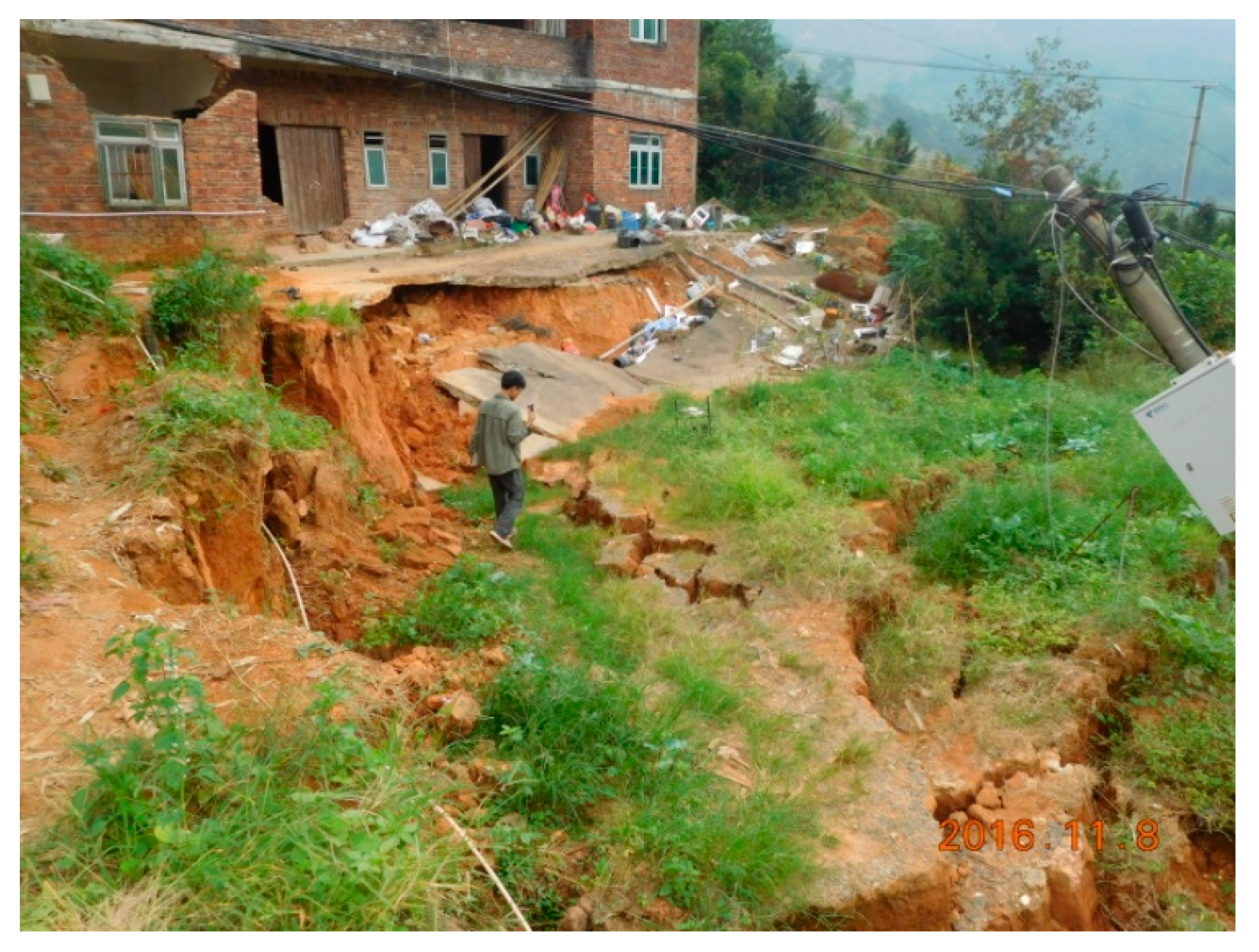
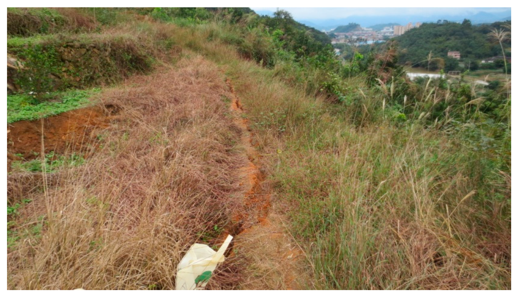
For a recent failed slope in Lengshuicun, Yongchun County, China, as reported in reference [12], the XGBoost–PSO–SVR model established in this study was used for comparison. Since the opening width at the rear edge of the slide mass of this slope was approximately 0.3 to 1 m, the main crack width was taken as 1.0 m. Moreover, since the rear edge of the slope body had already moved down as a whole by approximately 2 to 2.5 m, the main crack depth was taken as 2.5 m. Since there was rainfall from 4–7 November 2016, with a total rainfall of 126.1 mm, the rainfall duration was taken as 4 days, and the rainfall intensity was taken as 31.525 mm/day. According to the field investigation, as shown in Figure 8 and Figure 9, the crack area ratio at the top of the slope was estimated to be 20%, and the crack area ratio on the surface of slope was taken as 10%. The values of the other parameters are shown in

Table 6. Parameter values for evaluating slope stability.

Parameter	Value	Parameter	Value
H/m	38	Ir/(mm·d−1)	31.525
β/(°)	32.2	Wc/m	0.65
c/kPa	25	Dc/m	2.5
φ/(°)	24	Rt/%	20
γ/(kN·m−3)	18.8	Rf/%	10
Dr/d	4	-	-

.

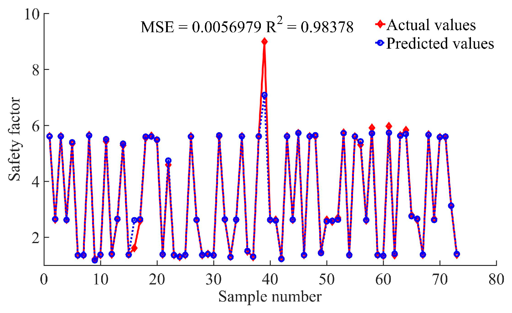
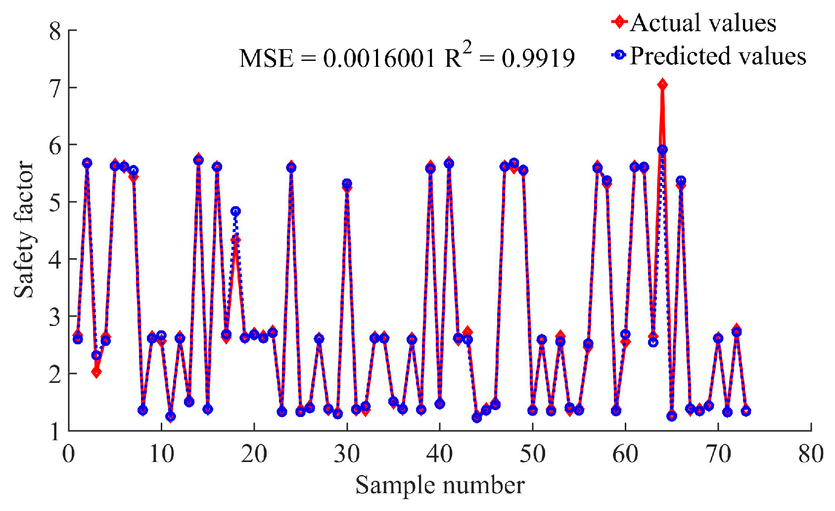
The parameters listed in Table 6 were input into the XGBoost–PSO–SVR model for prediction, and the results are shown in Figure 10.

It is evident from Figure 10 that the model predicted the 74th sample for this slope, with a value of 0.966. According to the Technical Code for Building Slope Engineering of China (GB50330-2013) [45], the stability state of this slope was unstable. According to the reference [12], the soil at the front edge of the slope moved forward by approximately 0.5 m from 4 to 7 November 2016, verifying the accuracy of the XGBoost–PSO–SVR model. The primary cause of the slope failure was the intense rainfall, which significantly increased the pore water pressure and reduced the shear strength of the soil. The total rainfall of 126.1 mm over the four-day period led to increased pore water pressure and soil saturation, which in turn reduced the effective stress and shear strength of the soil. The infiltration of rainwater into the slope body also increased the pore water pressure, particularly in the slip zone, leading to a decrease in the effective normal stress, thus reducing the soil’s resistance to slide. The high rainfall amount caused the soil to become saturated, further reducing its shear strength and increasing the likelihood of slope failure. These conditions collectively led to the slope failure. The safety factors obtained by using XGBoost, PSO–SVR, DT, KNN, NB, and RF for this slope are shown in

Table 7. Comparisons of safety factors predicted using various models.

Machine Learning Model	Predicted Value	Stability State	Simulation Results	Deviation
XGBoost–PSO–SVR	0.966	Unstable	0.988	0.022
XGBoost	1.005	Under stable		0.017
PSO–SVR	0.958	Unstable		0.030
DT	1.009	Under stable		0.021
KNN	0.955	Unstable		0.033
NB	1.024	Under stable		0.036
RF	1.017	Under stable		0.029

.

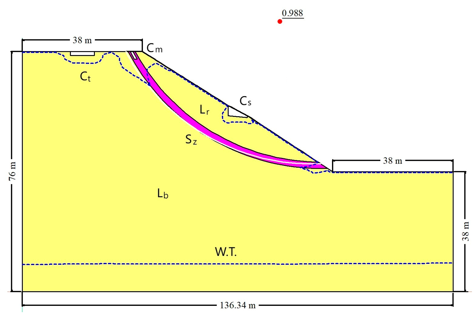
The numerical analysis of this slope using the software GeoStudio yielded a safety factor of 0.988, as shown in Figure 11. It is evident from Table 7 that the deviation between the predicted value obtained using XGBoost–PSO–SVR and the numerical analysis value was 0.022. Although this deviation was larger than that of XGBoost and DT, the prediction values of XGBoost and DT were both greater than 1. According to the Technical Code for Building Slope Engineering of China, the stability state of this slope should be judged as under stable, which did not match the actual situation of the slope slide. Therefore, in general, when compared with other methods, the prediction of XGBoost–PSO–SVR was closer to the actual situation.

5. Conclusions

(1)

By comparing the MSE and R2 indicators of the models, the XGBoost–PSO–SVR combined algorithm reduced the mean squared error by 71.9% and 57.8% compared to the individual XGBoost and PSO–SVR methods, respectively, and increased the accuracy of the dependent variable explanation by 0.83% and 0.69%, respectively. This model exhibited significant advantages in training accuracy and fitting effect. Moreover, when compared with the four single models, i.e., DT, NB, RF, and KNN, the XGBoost–PSO–SVR combined algorithm achieved the best training effect.

(2)

When the XGBoost–PSO–SVR combined algorithm was used to predict the stability of a recent failed slope in Lengshuicun, Yongchun County, from 4 to 7 November 2016, the predicted safety factor was 0.966, indicating that the slope was in an unstable state. This prediction result was consistent with the actual situation.

(3)

Due to the limitation of workload, this study simplified the cracks on the slope in the numerical simulation, considering only the main crack in the slip zone, the crack at the top of the slope, and the crack on the surface of slope. Moreover, the influence of groundwater and the spatial variability of slope parameters were not considered, which might result in differences between the predicted situation and the actual situation. Future research will focus on reasonably considering the impact of the above factors on the stability of recent failed slopes.

References

1. Yang, X.; Zhu, P.; Dou, X.; Yuan, Z.; Zhang, W.; Ding, B. Resurrection deformation characteristics and stability of Jiangdingya ancient landslide in Zhouqu, Gansu Province. Geol. Bull. China 2024, 43, 947–957. [Google Scholar]
2. Hu, G.; Liu, W.; Yan, Y.; Fan, X.; Zhang, Y.; Du, G.; Xiong, H.; Wang, M.; Yu, T. Reactivation characteristics and river blocking outburst simulation analysis of Sela ancient landslide in the upper reaches of Jinsha River. Acta Geol. Sin. 2024, 51, 160–170. [Google Scholar] [CrossRef]
3. Zhu, S.; Yin, Y.; Tie, Y.; Sa, L.; Gao, Y.; He, Y.; Zhao, H. Deformation characteristics and reactivation mechanism of giant ancient landslide in Wumeng mountain area: A case study of the Daguan ancient landslide. Chin. J. Geotech. Eng. 2025, 47, 305–314. Available online: http://kns.cnki.net/kcms/detail/32.1124.TU.20240522.0847.004.html (accessed on 25 February 2025).
4. Frink, N.T.; Pirzadeh, S.Z.; Parikh, P.C.; Pandya, M.J.; Bhat, M.K. Resurrection mechanism of retrogressive ancient landslide under cutting action: An example of an ancient landslide on National Way S206. Science Technol. Eng. 2023, 23, 15002–15009. [Google Scholar]
5. Fabrizio, B.; Guido, A.; Domenico, A.; Piero, F.; Matteo, G.; Gilberto, P. Landslide susceptibility analysis with artificial neural networks used in a GIS environment. Adv. Sci. Technol. Innov. 2024, 18, 291–294. [Google Scholar]
6. Liu, T.; Zhang, M.; Wang, L.; Yang, L.; Yin, B. Formation and evolution mechanism of the ancient landslide and stability evaluation of the accumulation body in Jiangdingya, Zhouqu County, Guansu Province. Bull. Geol. Sci. Technol. 2024, 43, 266–278. [Google Scholar]
7. Zhao, W.; Cao, J.; Guo, C.; Liu, J.; Yang, Z.; Wei, C.; Wu, R. Developmental characteristics and stability simulation of Yangpo Village large-scale ancient landslides in Minxian County, Gansu Province. Geol. Bull. China 2024, 43, 1869–1880. [Google Scholar]
8. Qiu, Z.; Guo, C.; Wu, R.; Jian, W.; Ni, J.; Zhang, Y.; Min, Y. Development Characteristics and Stability Evaluation of the Shadingmai Large-scale Ancient Landslide in the Upper Reaches of Jinsha River, Tibetan Plateau. Geoscience 2024, 38, 451–463. [Google Scholar]
9. Zhou, H.; Xiao, Q.; Peng, Y.; Li, C.; Qiu, Q. Stability analysis and engineering control plan optimization for secondary landslide of Gaokanzi in Enshi Xintang. J. Shenyang Univ. Nat. Sci. 2020, 32, 147–152. [Google Scholar]
10. Wang, K.; Chang, J.; Li, X.; Zhu, W.; Lu, X.; Liu, H. Mechanistic analysis of loess landslide reactivation in northern Shaanxi based on coupled numerical modeling of hydrological processes and stress strain evolution: A case study of the Erzhuangke landslide in Yan’an. Chin. J. Geol. Hazard Control. 2023, 34, 47–56. [Google Scholar]
11. Wang, J.; Cheng, Q.; Li, X.; Liu, N.; Zhang, P. Deformation and instability analysis of the transformed secondary landslide—A case of the RK24 landslide in Yuqing-Kaili expressway. Sci. Technol. Eng. 2020, 20, 89–95. [Google Scholar]
12. Chen, Z.; Dai, Z.; Jian, W. Cloud model for stability evaluation of recently failed soil slopes based on weight inversion of influencing factors. Chin. J. Geol. Hazard Control. 2023, 34, 125–133. [Google Scholar]
13. Zhang, L.; Jiang, X.; Sun, R.; Gu, H.; Fu, Y.; Qiu, Y. Stability analysis of unsaturated soil slopes with cracks under rainfall infiltration conditions. Comput. Geotech. 2024, 165, 105907. [Google Scholar] [CrossRef]
14. Tang, L.; Yan, Y.; Zhang, F.; Li, X.; Liang, Y.; Yan, Y.; Zhang, H.; Zhang, X. A case study for analysis of stability and treatment measures of a landslide under rainfall with the changes in pore water pressure. Water 2024, 16, 3113. [Google Scholar] [CrossRef]
15. Wei, X.; Ren, W.; Xu, W.; Cai, S.; Li, L. A Modified Method for Evaluating the Stability of the Finite Slope during Intense Rainfall. Water 2024, 16, 2877. [Google Scholar] [CrossRef]
16. Zheng, D.; Pan, M.; Gao, M.; Min, C.; Li, Y.; Nian, T. Multi-factor risk assessment of landslide disasters under concentrated rainfall in Xianrendong National Nature Reserve in southern Liaoning Province. Bull. Geol. Sci. Technol. 2025, 44, 48–58. [Google Scholar] [CrossRef]
17. Ma, H.; Wu, R.; Zhao, W.; Wang, J.; Qi, C.; Deng, P.; Li, Y. Development characteristics and reactivation deformation mechanism of the Lumai landslide in Shannan City, Xizang. Chin. J. Geol. Hazard Control. 2024, 35, 32–41. [Google Scholar]
18. LI, T.; Yuan, S.; Xu, J.; Hu, X.; Li, P. Two different types of models for stability assessment of rainfall triggered shallow landslides—Discuss with the paper risk assessment of Shallow Loess Landslides. Mt. Res. 2023, 41, 916–925. [Google Scholar]
19. Khalil, A.N.; Medeiros, S.; Allan, E.; Santos, D.S.; Denise, D.F. Assessment of mine slopes stability conditions using a decision tree approach. REM Int. Eng. J. 2023, 76, 71–78. [Google Scholar]
20. Jari, A.; Achraf, K.; Soufiane, H.; Elmostafa, B.; Sabine, M.; Amine, J.; Hassan, M.; Abderrazak, E.; Ahmed, B. Landslide susceptibility mapping using multi-criteria decision-making (MCDM), statistical, and machine learning models in the Aube Department, France. Earth 2023, 4, 698–713. [Google Scholar] [CrossRef]
21. Feezan, A.; Tang, X.; Qiu, J.; Piotr, W.; Mahmood, A.; Irfan, J. Prediction of slope stability using Tree Augmented Naive-Bayes classifier: Modeling and performance evaluation. Math. Biosci. Eng. 2022, 19, 4526–4546. [Google Scholar]
22. Yang, L.; Cui, Y.; Xu, C.; Ma, S. Application of coupling physics–based model TRIGRS with random forest in rainfall-induced landslide-susceptibility assessment. Landslides 2024, 21, 2179–2193. [Google Scholar] [CrossRef]
23. Fossat, E.; Aristidi, E.; Azouit, M.; Vernin, J.; Agabi, A.; Trinquet, H. Landslide susceptibility evaluation model based on XGBoost. Sci. Technol. Eng. 2022, 22, 10347–10354. [Google Scholar]
24. Das, S.K.; Pani, S.K.; Padhy, S.; Dash, S.; Acharya, A.K. Application of machine learning models for slope instabilities prediction in open cast mines. Int. J. Intell. Syst. Appl. Eng. 2023, 11, 111–121. [Google Scholar]
25. Cao, F.; Li, P.; Zhan, T.; Sun, X.; Zhang, Y. Risk prediction model of collapse and rockfall based on XGBoost and its application in highway engineering in complex mountain area. Transp. Technol. Manag. 2024, 5, 1–4. [Google Scholar]
26. Xu, J.; Hou, X.; Wu, X.; Liu, Y.; Sun, G. Slope displacement prediction using MIC-XGBoost-LSTM model. China J. Highw. Transp. 2024, 37, 38–48. [Google Scholar]
27. Ren, W.; Yang, X.; Feng, Y.; Yang, L.; Wei, J. Slope deformation prediction of SSA-SVR model based on GNSS monitoring. Saf. Environ. Eng. 2024, 31, 160–169. [Google Scholar]
28. Liu, X.; Liu, Z.; Ma, L.; Ren, K.; Wang, X. Slope stability coefficient prediction and variable analysis based on Support Vector Machine. J. Water Resour. Archit. Eng. 2023, 21, 172–178. [Google Scholar]
29. Lin, Y.; Xiong, J.; Xing, H.; Ning, X. Research on carbon emission prediction method of expressway construction based on XGBoost-SVR combined model. J. Cent. South Univ. 2024, 55, 2588–2599. [Google Scholar]
30. Ning, Y.; Cui, X.; Cui, J. Deformation prediction of open-pit mine slope based on ABC-GRNN combined model. Coal Geol. Explor. 2023, 51, 65–72. [Google Scholar]
31. Meng, Z.; Hu, Y.; Jiang, S.; Zheng, S.; Zhang, J.; Yuan, Z.; Yao, S. Slope Deformation Prediction Combining Particle Swarm Optimization-Based Fractional-Order Grey Model and K -Means Clustering. Fractal Fract. 2025, 9, 210. [Google Scholar] [CrossRef]
32. Wang, P. Study on stability prediction of high cutting slope based on GM-RBF combination model. Build. Struct. 2021, 51, 140–145. [Google Scholar]
33. Engineering Geology Manual Editorial Committee. Engineering Geology Manual, 5th ed.; Architecture & Building Press: Beijing, China, 2018. [Google Scholar]
34. Tang, H. Study on Instability Mechanism of Gently Inclined Soil Slope and Treatment Method of Gravel-Blind Ditch; Southwest University of Science and Technology: Mianyang, China, 2021. [Google Scholar]
35. Ren, S.; Zhang, Y.; Xu, N.; Wu, R.; Liu, X. Mobilized strength of sliding zone soils with gravels in reactivated landslides. Rock Soil Mech. 2021, 42, 863–873+881. [Google Scholar]
36. Huang, K. Stability prediction of reservoir slope based on GWO-XGBoost-SHAP. Sichuan Water Resour. 2024, 45, 46–51. [Google Scholar]
37. Xu, J.; Hou, X.; Wu, X.; Liu, Y.; Sun, G. Research on slope displacement prediction based on MIC-XGBoost-LST model. China J. Highw. Transp. 2024, 37, 38–48. [Google Scholar]
38. Hao, J.; Wei, X.; Wang, F. Slope reliability analysis based on MABC-SVR. J. Xi’an Univ. Archit. Technol. 2020, 52, 161–167. [Google Scholar]
39. Li, H.; Dai, S.; Zheng, J. Subsidence prediction of high-fill areas based on InSAR monitoring data and the PSO-SVR model. The Chinese J. Geol. Hazard Control. 2024, 35, 127–136. [Google Scholar]
40. Li, Q.; Pei, H.; Song, H.; Zhu, H. Prediction of slope displacement based on PSO-SVR-NGM combined with Entropy Weight Method. J. Eng. Geol. 2023, 31, 949–958. [Google Scholar]
41. Kennedy, J.; Eberhart, R. Particle swarm optimization. In Proceedings of the International Conference on Neural Networks, Perth, WA, Australia, 27 November–1 December 1995; IEEE: Piscataway, NJ, USA, 1995; pp. 1942–1948. [Google Scholar]
42. Eberhart, R.; Kennedy, J. A new optimizer using particle swarm theory. In Proceedings of the Mhs95 Sixth International Symposium on Micro Machine & Human Science, Nagoya, Japan, 4–6 October 1995; IEEE: Piscataway, NJ, USA, 1995; pp. 39–43. [Google Scholar]
43. Hu, S.; Li, Y.; Shan, C.; Xue, X.; Yang, H. Research on slope stability based on improved PSO-BP neural network. J. Disaster Prev. Mitig. Eng. 2023, 43, 854–861. [Google Scholar]
44. Zhang, Y.; Fu, M.; Wang, P.; Liang, J.; Guo, D. Slope stability analysis model based on PSO-RVM. Sci. Technol. Eng. 2023, 23, 8370–8376. [Google Scholar]
45. GB 50330-2013; Technical Code for Building Slope Engineering of China. Ministry of Housing and Urban-Rural Development of the People’s Republic of China. Architecture & Building Press: Beijing, China, 2013.
Figure 1. Schematic diagram of the numerical model.
Water 17 01920 g001
Figure 2. Relationship curve between matric suction and volumetric water content of slide soil.
Water 17 01920 g002
Figure 3. Relationship curve between matric suction and water X-conductivity of slide soil.
Water 17 01920 g003
Figure 4. Comparison between predicted values of the XGBoost model and actual values.
Water 17 01920 g004
Figure 5. Comparison between predicted values of the PSO–SVR model and actual values.
Water 17 01920 g005
Figure 6. Comparison between predicted values of the XGBoost–PSO–SVR model and actual values.
Water 17 01920 g006
Figure 7. Comparison between predicted values of four single-machine learning models and true values. (a) DT; (b) KNN; (c) NB; (d) RF.
Water 17 01920 g007
Figure 8. Downward platforms at the rear of the recent landslide.
Water 17 01920 g008
Figure 9. A tensile crack at the rear edge of slope.
Water 17 01920 g009
Figure 10. Predicted results of the XGBoost–PSO–SVR model.
Water 17 01920 g010
Figure 11. Numerical analysis result of slope.
Water 17 01920 g011