Article

Understanding Hydrological Responses to Land Use and Land Cover Change in the Belize River Watershed

by
Nina K. L. Copeland
1,2,
Robert E. Griffin
1,2,
Betzy E. Hernández Sandoval
1,2,*,
Emil A. Cherrington
1,2,
Chinmay Deval
1,2 and
Tennielle Hendy
3
1
Department of Atmospheric and Earth Science, University of Alabama in Huntsville, Huntsville, AL 35899, USA
2
SERVIR Science Coordination Office, NASA Marshall Space Flight Center, Huntsville, AL 35805, USA
3
National Hydrological Service, Ministry of Climate Change, Sustainable Development, and Solid Waste Management, Belmopan, Belize
*
Author to whom correspondence should be addressed.
Water 2025, 17(13), 1915; https://doi.org/10.3390/w17131915 (registering DOI)
Submission received: 16 May 2025 / Revised: 19 June 2025 / Accepted: 23 June 2025 / Published: 27 June 2025
(This article belongs to the Special Issue Applications of Remote Sensing and GISs in River Basin Ecosystems)

Abstract

Increasing forest destruction from land use and land cover change (LULCC) has altered catchment hydrological processes worldwide. This trend is also endemic to the Belize River Watershed (BRW), a significant source of land and water resources for Belize. This study aims to understand LULCC impacts on BRW hydrological responses from 2000 to 2020 by applying the widely used Soil and Water Assessment Tool (SWAT). This study identified historical trends in LULCC in the BRW and explored an alternative 2020 land cover scenario to elucidate the role of protected forests for hydrological response regulation. A SWAT model for the BRW was developed at the monthly timescale and calibrated on in situ streamflow using SWAT Calibrations and Uncertainty Programs (SWAT-CUP). The results showed that the BRW SWAT model performed satisfactorily for streamflow simulation at the Benque Viejo (BV) gauge station but performed variably at the Double Run (DR) gauge station. Overall, the findings revealed watershed-level increases in monthly average sediment yield (34.40%), surface runoff (24.95%), streamflow (16.86%), water yield (16.02%), baseflow (11.58%), and percolation (3.40%), and decreases in monthly average evapotranspiration (ET) (3.52%). In conclusion, the BRW SWAT model is promising for uncovering the hydrological impacts of LULCCs with opportunities for further model improvement.

1. Introduction

Land use and land cover change (LULCC) from the growing demand for natural capital and anthropogenic interference increasingly threatens ecosystems relied upon for human livelihoods [1,2,3]. From 2001 to 2015, forest destruction led to a loss of 314 Mha of the world’s tree cover [4]. The leading cause of tree cover loss during this period was commodity-driven deforestation, which accounted for approximately 27% of the global tree cover loss [4]. Deforestation related to forestry, shifting agriculture, and wildfires were also significant contributors [4]. Previous research suggests forests provide vital ecosystem services such as water quality regulation via nutrient and sediment filtration [5,6,7], erosion control and runoff reduction [8,9,10], groundwater recharge facilitation [11,12], and flood protection [13,14]. The replacement of forests for agricultural purposes can alter watershed hydrological responses by changing evapotranspiration (ET) fluxes [15], streamflow quantity [16], and nutrient and sediment loading [17,18].
Various scientific studies have investigated the impacts of LULCCs on watershed hydrological responses. Rápalo et al. [19] evaluated the effects of land cover and land use scenarios on streamflow regimes in the Mortes River Basin, Brazil using the Model for Large Basins. This study found that scenarios containing higher concentrations of agriculture and pasturelands led to increased maximum flows and reduced minimum flows [19]. Sadhwani et al. [20] used the Soil and Water Assessment Tool (SWAT) to analyze the impact of historical and future LULCCs on streamflow and sediment yield in the Periyar River Watershed, India. This study found increases in subwatershed-level surface runoff and sediment yield due to expanding urban areas and reduced forest coverage and plantations [20]. SWAT was also used by Ware et al. [21] to determine LULCC impacts on watershed hydrology in the Anyang Watershed, South Korea. Due to the expansion of agricultural lands, pasturelands, and urban areas from 2000 to 2022, groundwater recharge in the catchment decreased over time [21]. The effects of LULCCs on hydrological responses reported in the previous studies demonstrate the increasing influence of human activities on watershed health and dynamics.
Belizean watersheds are indicative of the growing global trend in LULCC-related forest replacement. Belize is a heavily forested Central American nation containing a large portion of protected landscape; however, evolving land use and land cover trends threaten the health of the nation’s watersheds. The Belize River Watershed (BRW) is the nation’s largest watershed, providing drinking water to around one-third of the nation’s population [22]. Agricultural expansion has been identified as a major threat to forests and water resources in the region due to deforestation, clear-cutting, sedimentation, and nutrient loading [22,23,24,25,26,27,28]. These activities threaten drinking water quality for rural communities that rely upon rudimentary water filtration systems [24,29]. Agricultural and logging demands for land and natural resources also put forests in protected areas at risk for deforestation and degradation [22,23,25,30,31].
Improving the understanding of anthropogenic impacts on natural capital using hydrological modeling is a growing field of research in Belize. Astmann et al. [29] employed SWAT to simulate the transport of glyphosate, a common herbicide, in the BRW. Their simulation predicted elevated pesticide concentrations in a downstream subwatershed containing a significant contributor of glyphosate to the Belize River [29]. Cherrington et al. [24] employed the Non-Point Source Pollution and Erosion Comparison Tool (N-SPECT) and SWAT to evaluate climate change and LULCC impacts on water resources in Belizean watersheds. Their findings suggested that projected increases in deforestation could lead to an 85.2% increase in surface runoff from 2010 to 2050 under a wetter future climate or lead to a 12.1% decrease in runoff during the same period under drier future conditions [24]. Martín-Arias et al. [32] also used N-SPECT to identify the combined effect of projected LULCC and climate change on runoff and sediment yield in Belizean watersheds. Results from this study suggested that reduced projected deforestation in the BRW led to lower projected runoff volumes when isolated from climate effects [32]. These studies present a foundation for hydrological modeling applications in the BRW but provide further opportunities to explore the effects of LULCC on the watershed’s hydrological cycle.
Many studies have demonstrated the utility of SWAT for evaluating LULCC influences on hydrological responses in subtropical and tropical catchments [33,34,35,36,37,38,39,40,41,42,43,44,45,46,47]. Considering SWAT’s widespread usage in watersheds of similar climates and the model’s range of customizability, the present study was designed to assess the impact of LULCCs on hydrological responses in the BRW from 2000 to 2020 using SWAT. Hydrological components explored in this research include streamflow, water yield, sediment yield, surface runoff, baseflow, ET, and percolation. The following three research objectives were outlined for this study:
  • Calibrate and improve the accuracy of the SWAT model using in situ streamflow measurements and the SWAT Calibration and Uncertainty Programs (SWAT-CUP);
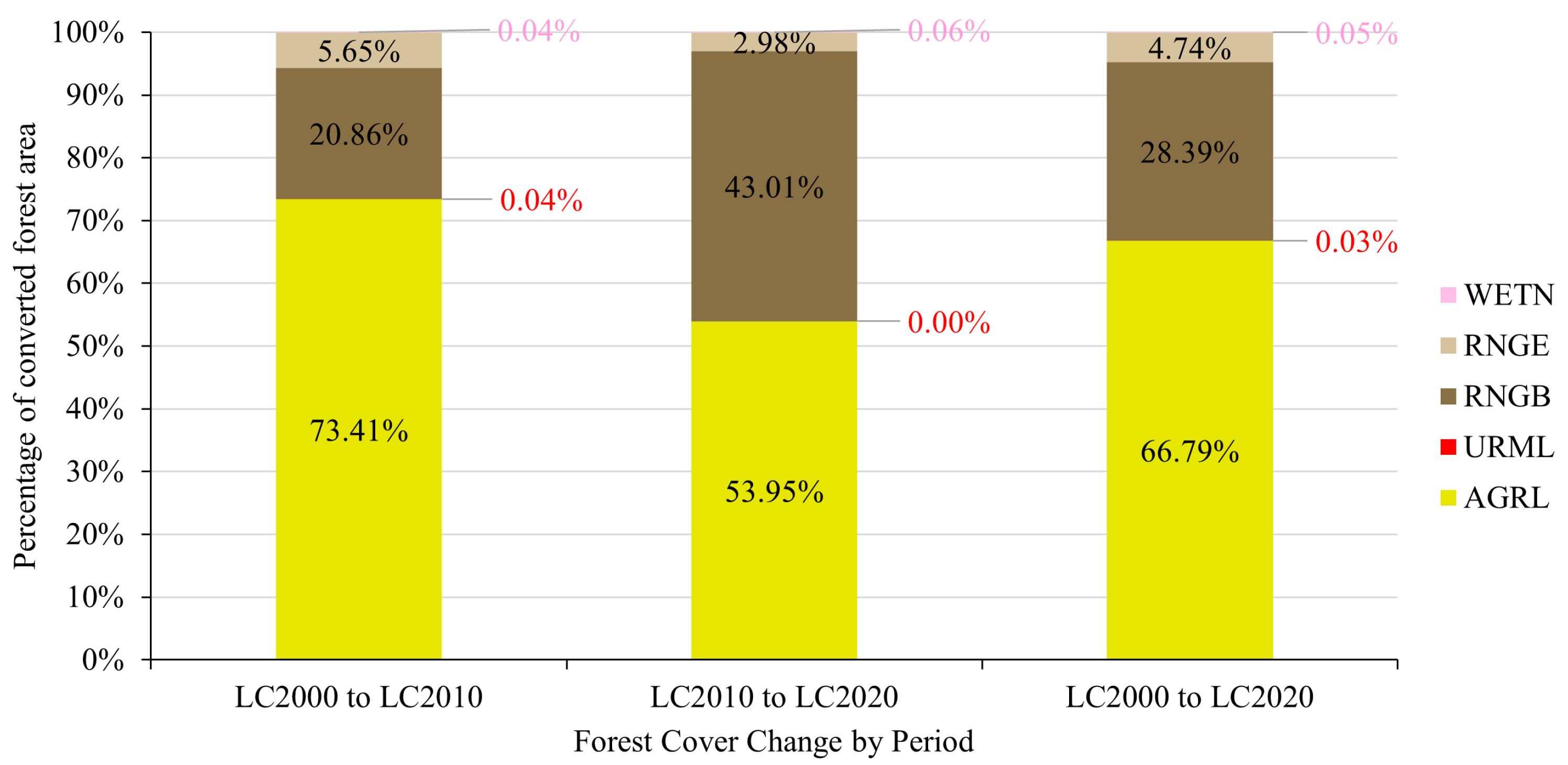
  • Investigate the predominant land use and land cover patterns replacing forests in the BRW;
  • Examine the changes in simulated hydrological responses at the watershed and subwatershed levels between three annual land cover datasets, (i.e., 2000, 2010, and 2020) and an alternative 2020 land cover scenario replacing agricultural lands in protected areas with evergreen forests.
To these authors’ knowledge, the present study is the first SWAT study to investigate the impacts of historical LULCC on hydrological responses focused on the full extent of the BRW. This study aims to elucidate the influence of human activities on hydrological regimes and examine the significance of protected areas for safeguarding vital forest stocks that stabilize hydrology in the region. The present study contributes to the current field of SWAT research by quantifying the effects of LULCC on watershed dynamics and building a foundation for water resource and sediment monitoring using hydrological models in the region.

2. Materials and Methods
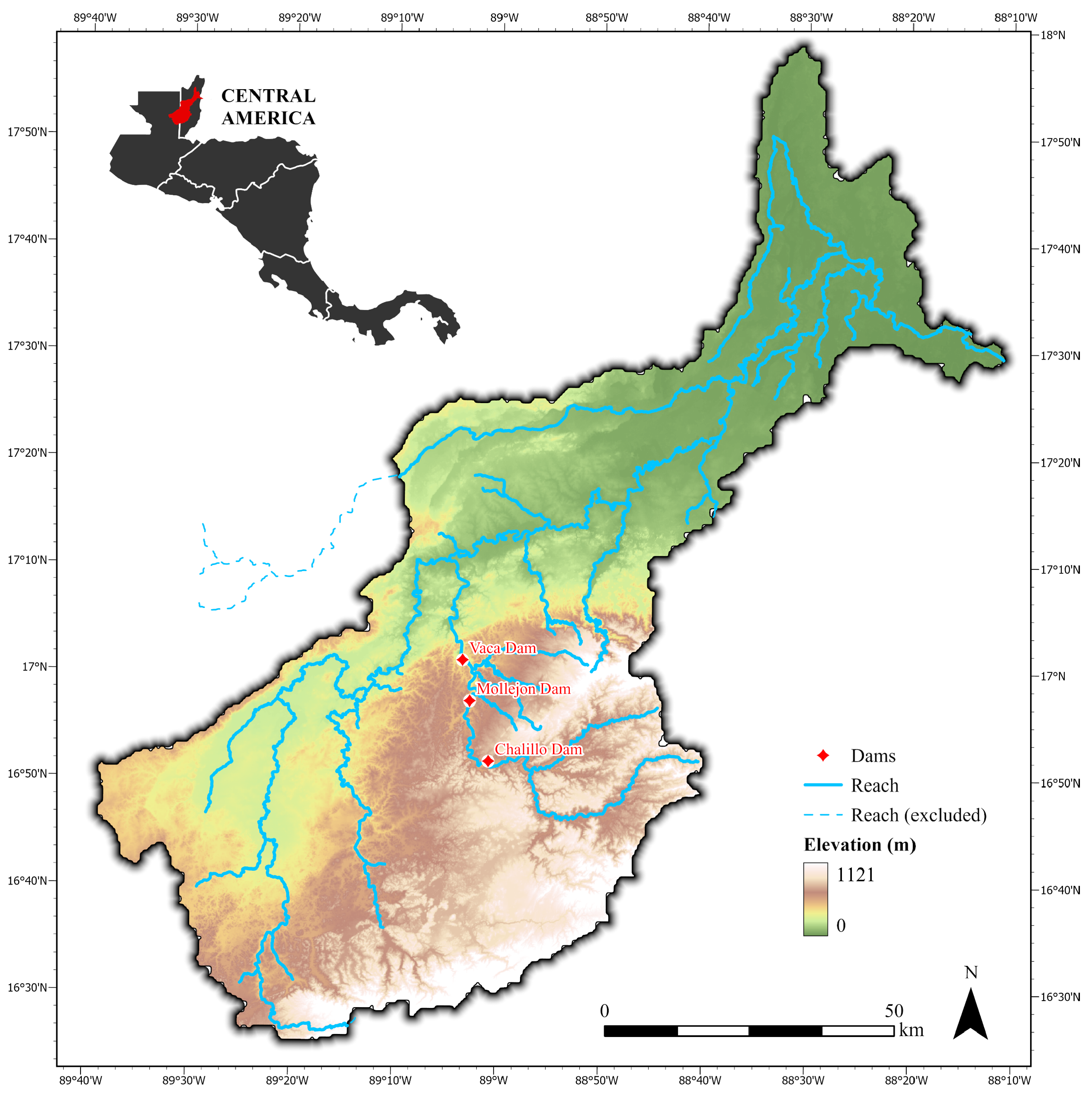
2.1. Study Area

The present study was conducted in the BRW (Figure 1), a transboundary catchment between Belize and Guatemala located between 17°58′ N, 88°9′ W and 16°25′ N, 89°38′ W. The BRW is the largest watershed in Belize and encompasses an area of approximately 8562 km2. The Belize River contains headwaters from the Mopan River and Macal River tributaries. The Mopan River originates in the western foothills of the Maya Mountains in Belize, and it stretches into Guatemala; its landscape is characterized by large swaths of agriculture and steeper slopes along the Maya Mountains. The Macal River drains from the Maya Mountains in western Belize and its catchment is heavily forested; however, forests in this region face threats from resource extraction and agricultural incursions [30]. The Macal River tributary also contains the Vaca, Mollejon, and Chalillo hydroelectric dams. Both rivers flow into the Belize River near San Ignacio, Belize, and the Belize River then discharges into the Caribbean Sea north of Belize City, Belize. Figure 1 depicts the extent of the BRW, its streams, and the associated dams.
The watershed’s climate is hot/humid and subtropical with distinct wet (May to November) and dry (December to April) seasons. Annual rainfall for the BRW ranges from 1600 mm to 2500 mm, with higher amounts falling in its upper reaches [48]. Annual temperatures range from 25 °C to 38 °C in the wet season and 16 °C to 28 °C in the dry season [48]. The watershed is largely forested with significant portions of terrain under protection, particularly in its upper reaches. Agricultural pressures are prevalent in the watershed’s upper Guatemalan reaches and its middle Belizean reaches. Wetlands and mangroves can be found in the lower reaches of the watershed. Permanent and seasonal wetlands are also found in Yaxhá-Nakum-Naranjo National Park, Guatemala [49].
As the largest watershed in Belize, at least 40% of the Belizean population live within the bounds of the BRW as of 2018 [50]. Over half of this population is rural [27,50]; however, there are various population centers throughout the BRW including Belmopan city, San Ignacio, and Benque Viejo del Carmen in Belize and Melchor de Mencos in Guatemala. Furthermore, a large Mennonite population in Spanish Lookout, Belize conducts significant large-scale agricultural activities in the region [51]. The soils in the BRW are predominantly made of cambisols [52,53], which can have a variable depth that reaches 25 cm in thickness and are in a transition stage of development between young soil and more mature soil [52,53]. However, soil characteristics are spatially variable throughout the soil profile and the watershed. The acidic, siliceous soils of the Maya Mountains are prone to erosion and composed of Paleozoic metamorphic and volcanic rocks with granitic intrusions [26,48]. In the middle reaches, the calcareous soils overlay Cretaceous limestones and dolomites, which have higher fertility and support agricultural stability [26,48]. The lower coastal reaches consist of Pleistocene alluvium deposits [48].

2.2. The SWAT Model

The SWAT model is an open-source, semi-physically based, continuous, semi-distributed hydrological model first developed by the United States Department of Agriculture Agricultural Research Service to model the impacts of management practices on watershed regimes [54]. The model has four main data inputs: land use, soil classes, elevation, meteorological forcing such as precipitation, air temperature, relative humidity/dewpoint temperature, wind speed, and solar radiation. The SWAT model includes components to simulate watershed processes such as water cycling, sediment yield and concentration, fertilizer and pesticide application, land management practices, nutrient cycling, and plant growth. The hydrological balances in SWAT are simulated on three spatial scales: basin level, sub-basin level, and hydrological response unit (HRU) level. HRUs are generated based on areas that share similar characteristics in land use, soil type, and slope. These HRUs are assumed to have homogeneous hydrological responses to changes in meteorological forcing. Generally, SWAT modeling can be performed at the daily, monthly, and annual temporal scales; however, some studies demonstrate sub-daily capacities for SWAT modeling [55,56,57].
To simulate hydrological balances in watersheds, SWAT uses the following equation:
S W t = S W 0 + i = 1 t ( R Q s r E T W s e e p Q g w ) ,
where S W t is final soil water depth (mm H2O); S W 0 is initial soil water depth (mm H2O); t is time (days); R is precipitation on day i (mm H2O); Q s r is surface runoff on day i (mm H2O); E T is ET on day i (mm H2O); W s e e p is percolation on day i (mm H2O); and Q g w is the return flow/baseflow on day i (mm H2O).
SWAT model calibration involves adjusting model inputs (i.e., model parameters) by comparing simulated results with in situ observations to improve model accuracy [58]. SWAT-CUP is a commonly used software for calibration. Various versions of the software exist such as SWAT-CUP 2012, SWAT-CUP 2019, SWATplus-CUP, and SWAT-CUP Premium. In this study, SWAT-CUP Premium was utilized for model calibration. SWAT-CUP Premium contains two calibration algorithms: Particle SWAT Organization (PSO) and SWAT Parameter Estimator (SPE) [59]. SPE is the successor to the widely used SWAT-CUP Sequential Uncertainty Fitting (SUFI-2) procedure, and various studies have found SUFI-2 to adequately perform model calibration using observed streamflow in tropical and subtropical catchments worldwide [29,35,41,43]. SPE is an iterative algorithm that uses a Latin hypercube program to sample parameters within preset ranges [59]. After sampling, the algorithm maps the target parameters while attempting to capture the in situ observations within the 95% confidence interval (95PPU) of the simulated results [59]. The algorithm’s output, the 95PPU band, is quantified and assessed using two statistics: p-factor and r-factor [59]. P-factor is the portion of observed data points that fall within the 95PPU band, and r-factor is the width of the 95PPU band [60]. These statistics may be used to perform uncertainty analysis in SWAT-CUP. Model performance in SWAT-CUP Premium can be assessed using 11 objective functions, or statistical measures, for comparing simulated results with observed data points [59]. SPE differs from SUFI-2 in that it allows for multi-objective functionality, where more than one objective function can be considered during the iterative calibration process [59]. In this study, we used SPE for model calibration, as its predecessor SUFI-2 has been successfully applied in various studies with similar catchment settings.

2.3. Data Acquisition and Preprocessing

Preprocessing of the spatial model inputs (i.e., digital elevation model (DEM), land cover, and soil map) was performed in ArcGIS Pro Ver 2.9.8. All geospatial datasets were projected in the NAD 1927 UTM Zone 16N projection and a cell resolution of 300 m was used. Ancillary datasets for the stream network, water bodies, protected area boundaries, and river stage were used for preprocessing and model setup.

2.3.1. Elevation Data and Stream Network
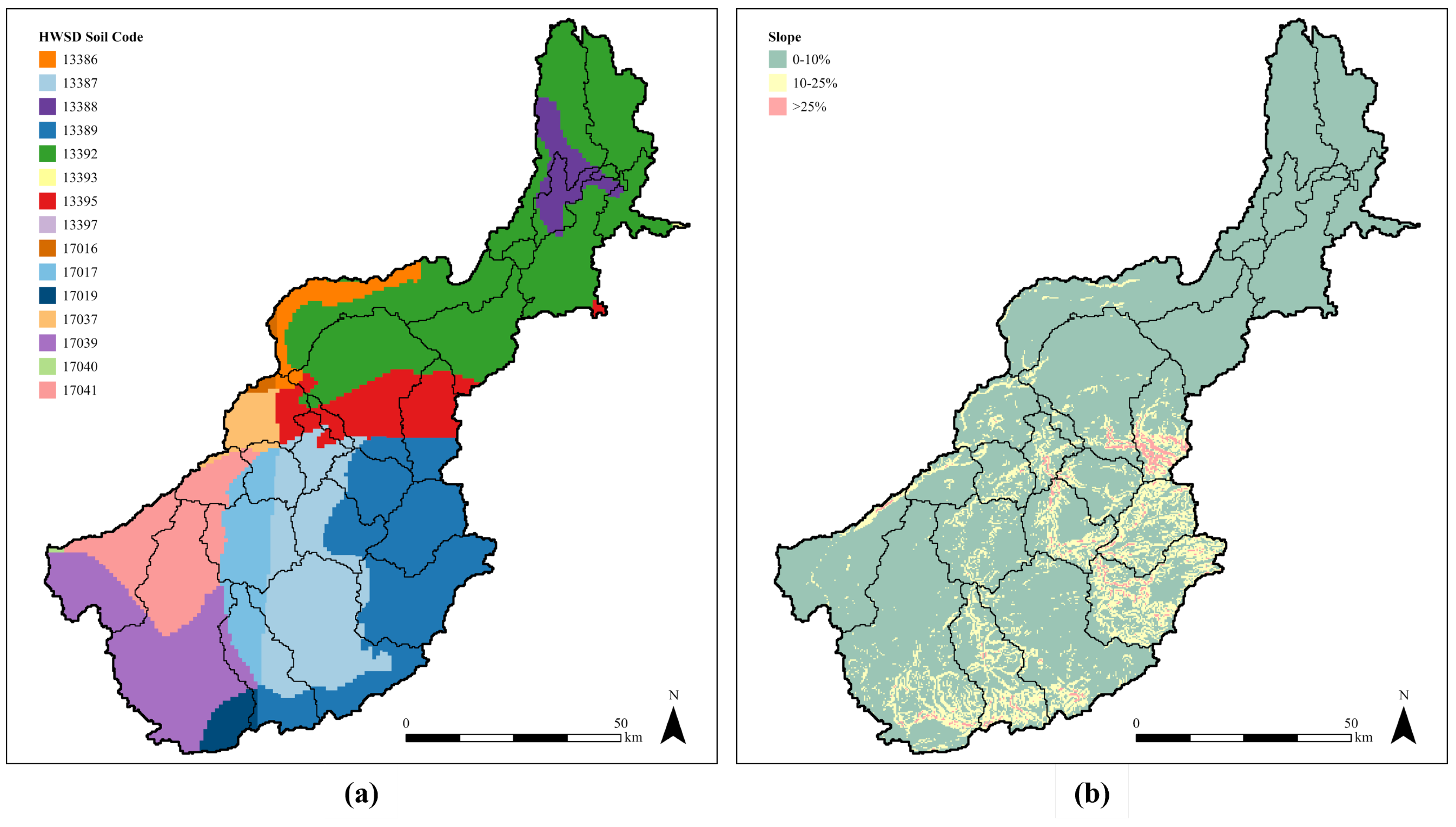
Four void-filled Shuttle Radar Topography Mission (SRTM) DEM tiles at 90 m resolution were collected from the United States Geological Survey’s (USGS) Earth Explorer for the elevation input [61]. The ease of accessibility and widespread usage of the STRM DEM for LULCC SWAT analyses made it an optimal candidate for elevation input in the BRW SWAT model [38,40,47,62,63]. To improve the representation of rivers in the DEM, the hydrographic network was ’burned into’ the DEM using the methodology outlined in Cherrington [64]. That hydrographic network data was based on map data provided by the U.K. Ordnance Survey, the Belize Land Information Centre, Mexico’s INEGI, and Guatemala’s National Geographic Institute.

2.3.2. Soil Data

A global soil map was collected from the Harmonized World Soil Database (HWSD) Ver 1.2 in the Food and Agriculture Organization of the United Nations (FAO) Soils Portal [53]. The HWSD is a commonly used soil map for simulating hydrological dynamics like streamflow and sediment yield with SWAT across global catchments [44,65,66]. The availability of the HWSD in SWAT format also improves its applicability for SWAT modeling [67]. Soil characteristics from the HWSD were appended to the SWAT User Soil Database to customize the model. Soil data for the topsoil (0 to 30 cm) and the subsoil (30 to 100 cm) were manually input into the database. Table 1 shows the 15 soil classes in the watershed and the percentage of watershed area representative of each class.

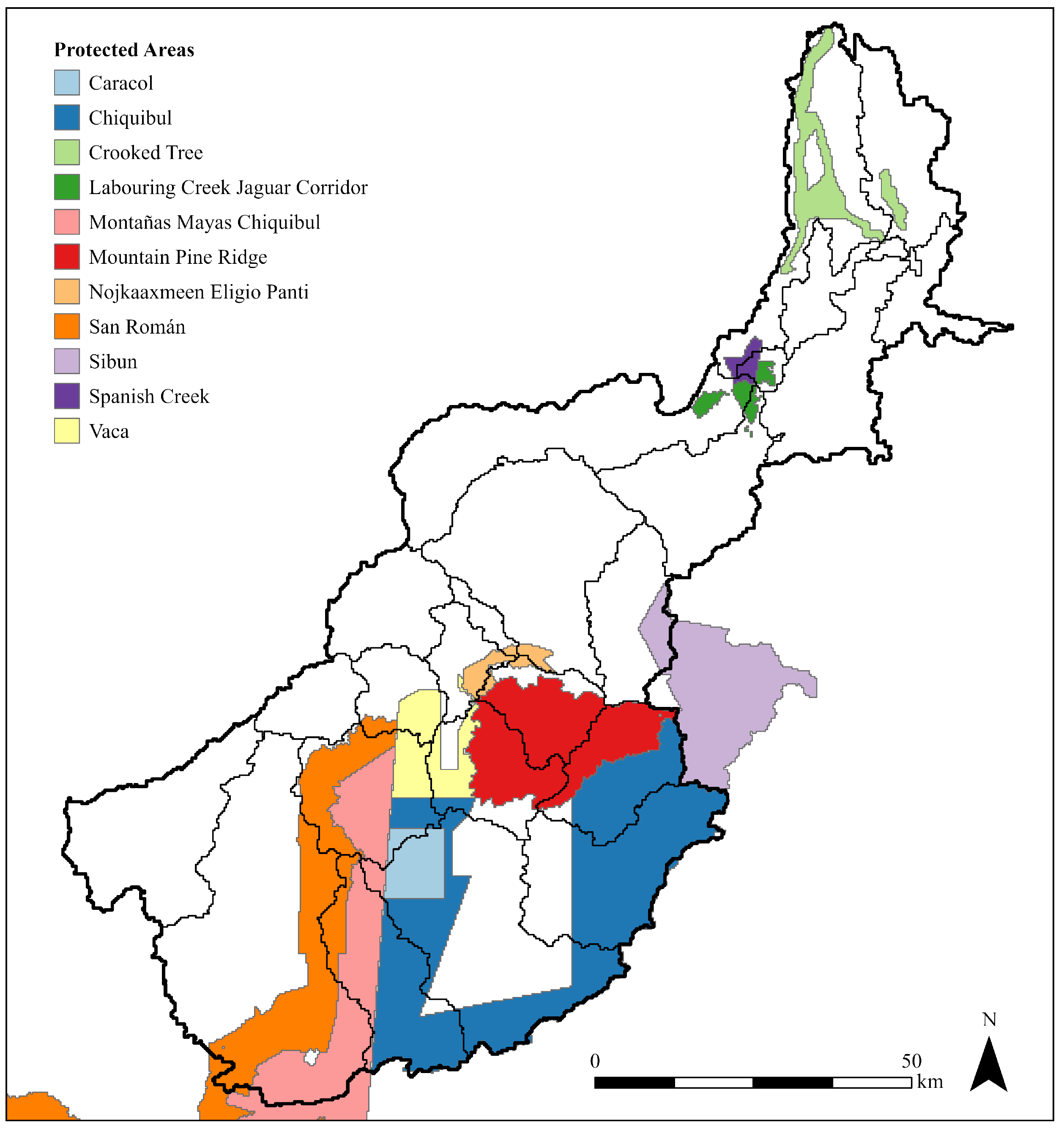
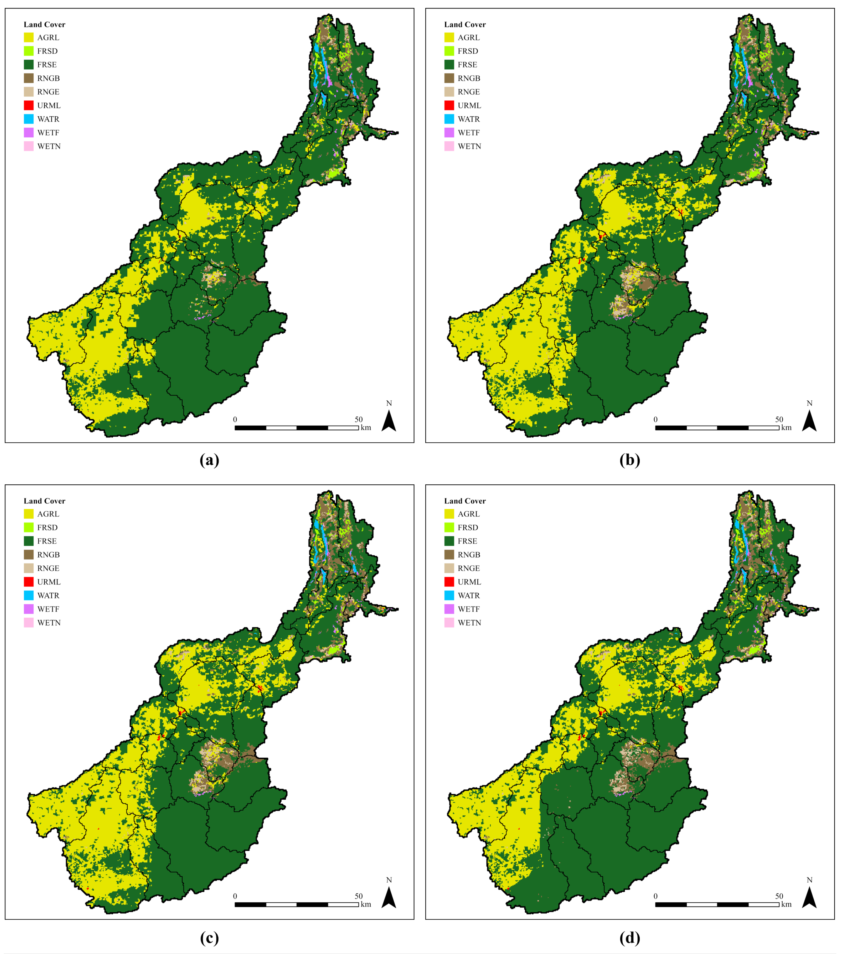
2.3.3. Land Cover and Protected Areas Data

Land cover data from the European Space Agency’s (ESA) Climate Change Initiative (CCI) was used because of its large period of availability and its capacity to cover the transboundary expanse of the study area. Land cover for 2000 and 2010 was acquired from Ver 2.0.7cds of the product, and land cover for 2020 was acquired from Ver 2.1.1 of the product [68,69]. Land cover datasets were converted to GeoTIFF format and clipped within a 2 km buffer of the watershed boundary. The land cover was then reclassified to align with SWAT land use classes. Table 2 shows the reclassified land cover classes.
Protected area boundaries from Belize and Guatemala were collected from Protected Planet to create the alternative 2020 scenario [70]. This scenario replaces agricultural cover within encroached protected areas in the actual 2020 land cover with evergreen forest cover. This scenario was created to understand the influence of forest cover in these areas on the watershed’s hydrology. Figure 2 shows the boundaries of the protected areas considered in this study.

2.3.4. Meteorological Data

Precipitation, temperature, and relative humidity measurements were obtained from the National Meteorological Service of Belize (NMSB) for sixteen manual and automatic stations across the BRW’s Belizean side. Due to the uneven spatial distribution of the stations as well as data gaps in the measured characteristics, it was necessary to incorporate the use of supplemental meteorological data from institutional and public databases. Daily precipitation and temperature data were available on the SWAT website from the Climate Hazards Group Infrared Precipitation with Stations (CHIRPS) and the Climate Hazards Group Infrared Temperature with Stations (CHIRTS-daily) [71,72]. CHIRPS and CHIRTS-daily were available in SWAT format and did not require preprocessing. Solar radiation and wind speed data were required to calculate ET with SWAT. Solar radiation and wind speed measurements were collected from the United States National Renewable Energy Laboratory’s Physical Solar Model Ver 3 from the National Solar Radiation Database (NSRDB) [73]. Like the soil data, preparation of meteorological data was also required for input into the SWAT database. Users can input monthly period averages for weather stations in the SWAT Weather Generator (WGEN) for long-term climate characteristics. Four manual stations in the watershed were selected for input into the WGEN based on data availability: NMSB Central Farm station, NMS Belmopan station, NMSB Punta Gorda International Airport (PGIA) station, and station SA_628835 from CHIRPS and CHIRTS-daily. The CHIRPS/CHIRTS-daily station closest to the centroid of the BV drainage basin was used to compensate for the absence of in situ stations in that region. Solar radiation and wind speed data for each WGEN station were aggregated into daily measurements for input into the database. After the preparation of all meteorological variables, the monthly period averages (1990 to 2020) of precipitation, minimum and maximum air temperature, solar radiation, relative humidity, and wind speed were calculated for each WGEN station using the WGNmaker4 Excel macro from the SWAT website [74]. Dewpoint temperature averages were derived in the WGNmaker4 Excel macro using relative humidity from the NMSB stations.

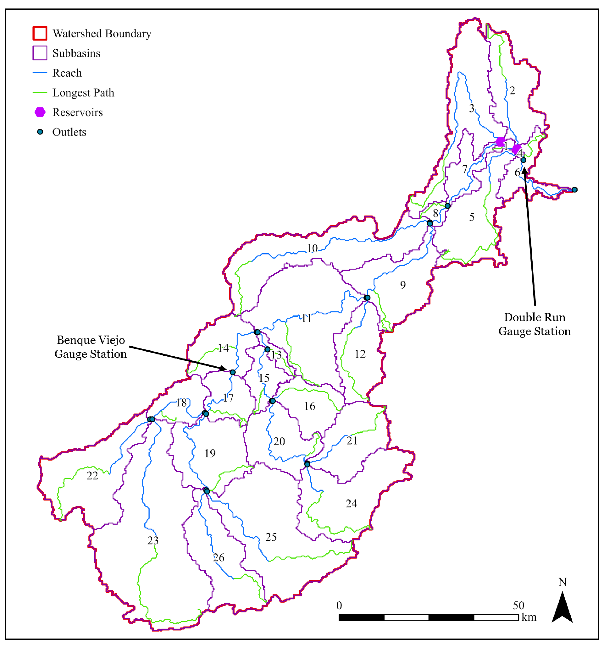
2.3.5. Hydrological Data

Daily average streamflow data from two gauge stations at the monthly time step were used for calibration and validation of the SWAT model: Double Run (DR) and Benque Viejo (BV). Streamflow and river stage data were provided by the National Hydrological Service of Belize (NHSB). The watershed boundary was delineated using HydroSHEDS’ DEM [75]. Two water body datasets were collected: one for Belize from the Biodiversity and Environmental Resource Data System of Belize (BERDS) and one for Guatemala from the World Bank Data Catalog [76,77]. When applicable, water body data was necessary for designating the fraction of reservoir/pond area and reservoir/pond volume for each sub-basin in the SWAT project database. In SWAT, reservoirs are defined as impoundments residing along the main river channel of a sub-basin [78]; in contrast, ponds are defined as sub-basin impoundments located outside the main channel [78]. Reservoirs and ponds may represent sinks for water flow in the catchment, and the inclusion of reservoirs and ponds in the SWAT model is significant for adequate simulation of streamflow contribution. The surface areas of reservoirs and ponds were available from the water body datasets; however, water body volume was unavailable. To calculate volume, depths were assumed using similar aquatic ecosystems from Pérez et al. [79], which surveyed water bodies across Mexico, Guatemala, and Belize. These assumed depths and the available surface areas were multiplied to calculate total reservoir/pond volumes.

2.4. SWAT Model Setup

For model setup, ArcSWAT 2012 in the ArcGIS Ver 10.8.2 interface was used. The setup methodology described below was repeated for the annual land cover datasets (2000, 2010, and 2020) and the 2020 reforestation scenario. These datasets are hereby referred to as LC2000, LC2010, LC2020, and LC2020PA, respectively. The first step was watershed delineation, which denotes the watershed’s boundary and the boundaries of its associated sub-basins (see Figure 3). For the elevation input, the preprocessed DEM was selected in the Watershed Delineation interface. A rasterized mask of the watershed boundary was selected to guide the watershed boundary delineation, and flow direction and flow accumulation were calculated by the model. After these steps, a streamflow network and outlet points were delineated. Outlet points were manually delineated for DR and BV to represent each station. The main outlet of the watershed was selected, after which the entire watershed boundary and its sub-basins were delineated. Twenty-six sub-basins were defined, and the total watershed area was calculated as 8743.23 km2. After watershed delineation, two reservoirs were specified: Jones Lagoon in sub-basin two and Spanish Creek and Northern Lagoon in sub-basin three. Figure 3 shows the boundary and sub-basins of the BRW as delineated in ArcSWAT.
Next, sub-basins were divided into HRUs. Lookup tables were created to reclassify land cover and soil types for HRU generation. Three slope classes were defined: 0–10% for gentle slopes, 10–25% for moderate slopes, and >25% for steep slopes. The four land cover datasets used in this research are shown in Figure 4. The distribution of soil types and slope classes is shown in Figure 5. HRU thresholds may be applied to combine smaller HRUs below the thresholds with larger HRUs. For this study, no thresholds were specified to preserve the greatest detail in HRU generation.
Next, weather inputs were selected. Two types of weather stations can be defined for sub-basins: individual weather stations and WGEN weather stations. Individual stations provide direct measurements of meteorological characteristics, and WGEN stations provide monthly period averages of climatic characteristics to interpolate missing weather data. For each station type, SWAT selects the station closest to a sub-basin’s centroid to represent its weather conditions. Twenty-six CHIRPS and CHIRTS-daily stations containing daily precipitation and temperature measurements were selected, and WGEN stations were defined for each sub-basin.
The Priestley–Taylor method was used to calculate potential ET (PET). Previous literature suggests that the Priestley–Taylor method is satisfactory for calculating PET in humid regions [80,81]. Priestley–Taylor PET is calculated using the following equation:
λ E T 0 = α · Δ Δ + γ · ( H N G ) ,
where λ is latent heat of vaporization (MJ/kg); E T 0 is potential ET (mm/day); α is a coefficient ( α = 1.28 ); Δ is the slope from the saturation vapor pressure-temperature curve, d e / d t (kPa/°C); γ is the psychrometric constant (kPa/°C); H N is the net radiation (MJ/m2/day); and G is the heat flux density to the ground (MJ/m2/day).
To calculate surface runoff, the initial runoff curve number (CN2) was calculated as a function of ET to reduce the overprediction of runoff in the default model. The SWAT theoretical documentation provides more information about the PET and CN2 methods [81]. Monthly simulations were performed for all land cover datasets from 1 January 2000 to 31 December 2020. Seventeen warm-up years were specified to ensure proper water cycling in the model before the period of interest, utilizing data available from the CHIRPS and CHIRTS-daily stations for the years 1983 to 1999.

2.5. Model Calibration and Validation

The present model was calibrated on streamflow measurements from BV, represented by the sub-basin 17 outlet point. This gauge station was selected for calibration because no major dams exist within its drainage basin. Dam activities may cause unnatural influences on streamflow, providing a challenge for streamflow calibration. Therefore, only parameters in the seven sub-basins draining into BV were altered during calibration. The model was calibrated from 1 January 2000 to 31 December 2006. SWAT calibration was performed using the SPE algorithm and its multi-objective functionality in SWAT-CUP Premium. Multi-objective functionality was used to consider three objective functions during SPE iterations: the coefficient of determination (R2), the Nash–Sutcliffe efficiency (NSE), and percent bias (PBIAS). R2 ranges from 0 to 1 and measures the proportion of variance between observed measurements and modeled results [58]. R2 values closer to 1 represent a better correlation between the observed and simulated data [58]. NSE ranges from −∞ to 1 and measures the fit of the observed versus the simulated data to the 1:1 line by comparing residual and observed data variances [58,82]. NSE values closer to 1 represent a better agreement between the observed and simulated data [58]. PBIAS ranges from −∞ to +∞ and measures the average deviation between the observed and simulated data points [58]. Negative PBIAS represent an overestimation bias and positive PBIAS represent an underestimation bias [58]; however, values closest to 0 are most desirable [58]. Table 3 was adapted from Houshmand Kouchi et al. [83] and Moriarsi et al. [58] and shows the model performance ratings for R2, NSE, and PBIAS used to assess the SWAT simulation in this study.
The following equations show how R2, NSE, and PBIAS were calculated:
R 2 = i = 1 n ( Q i o b s Q o b s ¯ ) ( Q i s i m Q s i m ¯ ) 2 i = 1 n ( Q i o b s Q o b s ¯ ) 2 · i = 1 n ( Q i s i m Q s i m ¯ ) 2 ; 0 R 2 1 ,
N S E = 1 i = 1 n ( Q i o b s Q i s i m ) 2 i = 1 n ( Q i o b s Q o b s ¯ ) 2 ; N S E 1 ,
P B I A S = i = 1 n ( Q i s i m Q i o b s ) · 100 i = 1 n ( Q i o b s ) ; P B I A S ,
where Q i o b s is the ith observed streamflow measurement, Q o b s ¯ is average observed streamflow, Q i s i m is the ith simulated streamflow measurement, Q s i m ¯ is the average simulated streamflow, and n is the total count of streamflow measurements.
The calibration methodology used in this study generally follows the steps outlined in Abbaspour et al. [84] who suggested applying parameter regionalization techniques to determine relevant model parameters. To determine the calibration parameters, 17 hydrologically influential parameters were selected for sensitivity analyses in SWAT-CUP Premium. Sensitivity analyses were used to determine the degree of model output change based on model inputs [58]. The most sensitive parameters were selected by performing four sensitivity analyses using parameter subsets based on the hydrological processes they impact. The categories for these subsets were ET, groundwater, surface runoff, and soil water. Parameters are considered sensitive when their p-value is less than 0.05 [59]. Large t-stat values are also indicative of a sensitive parameter [59]. Sensitive parameters are more likely to influence streamflow agreement between the simulated and observed measurements. Based on the four sensitivity analyses, the 11 parameters shown in Table 4 were selected for calibration.
The initial parameter ranges for the first SWAT-CUP Premium iteration are shown in Table 5. An iteration characterized a set of 500 model simulations and new parameter ranges were selected after each consecutive iteration. Every parameter aside from CANMX was calibrated across all soil types, land uses, and slope classes. Parallel processing functionality was utilized in SWAT-CUP Premium to decrease the processing time of the SWAT-CUP Premium iterations [85]. Subsequent iterations were performed until a satisfactory simulation was achieved based on the model performance ratings.
To validate the model, streamflow measurements from DR and BV were used. Despite influences from the Chalilo, Mollejon, and Vaca dams, DR is closest to the river’s mouth and represents streamflow contributions from most of the watershed’s drainage area. DR was represented by flow out of sub-basin four. In this study, validation at DR was used to determine if the parameters and their fitted values determined during BV calibration could be used to accurately simulate downstream flow. The validation period for BV and DR was 1 January 2007, to December 2013.
To validate the model, the model’s parameters were fitted during the calibration process. The primary soil class of the BV drainage basin was cambisols; therefore, soil parameters of soil types with the primary class of gleysols were not changed in the greater watershed.

2.6. Spatial Analysis of LULCCs Leading to Forest Cover Loss

To detect the spatial changes in land cover, a LULCC analysis was performed using the Change Detection Wizard in ArcGIS Pro Ver 3.3.0. The main LULCC of interest was the conversion of forest classes (i.e., evergreen forests, deciduous forests, and forested wetlands) to some other non-forest class. Annual land cover datasets were entered into the wizard in pairs. First, LC2000 and LC2010 were input to reveal forest cover losses during the first 10 years of the study period. A dataset containing the changes for that period was then produced. This process was repeated to reveal the spatial distribution of forest cover replacement from LC2010 to LC2020, LC2020 to LC2020PA, and LC2000 to LC2020PA. The Identity geoprocessing tool was used to overlay the change detection datasets with the BRW sub-basins to distinguish LULCCs by sub-basins. In the overlaid datasets from the Identity tool, the area in square kilometers of each unique land conversion was calculated using the Calculate Geometry Attributes geoprocessing tool. The area of each unique land conversion was then aggregated for the entire watershed and by sub-basin.

2.7. Analysis of Modeled Results

To determine the impacts of forest cover loss from LULCC on hydrological dynamics, the SWAT outputs for all four land cover simulations were analyzed on the monthly timescale from 2000 to 2020 using Microsoft Excel. For each scenario, the period averages of targeted hydrological dynamics for every month (i.e., January, February, etc.) were calculated and compared. For the entire watershed, the hydrological dynamics considered in this study were streamflow, water yield, sediment yield, surface runoff, ET, percolation, and baseflow. Three case studies were completed to analyze the localized impacts of forest cover loss on hydrological dynamics. For these case studies, three sub-basins were selected matching the following characteristics:
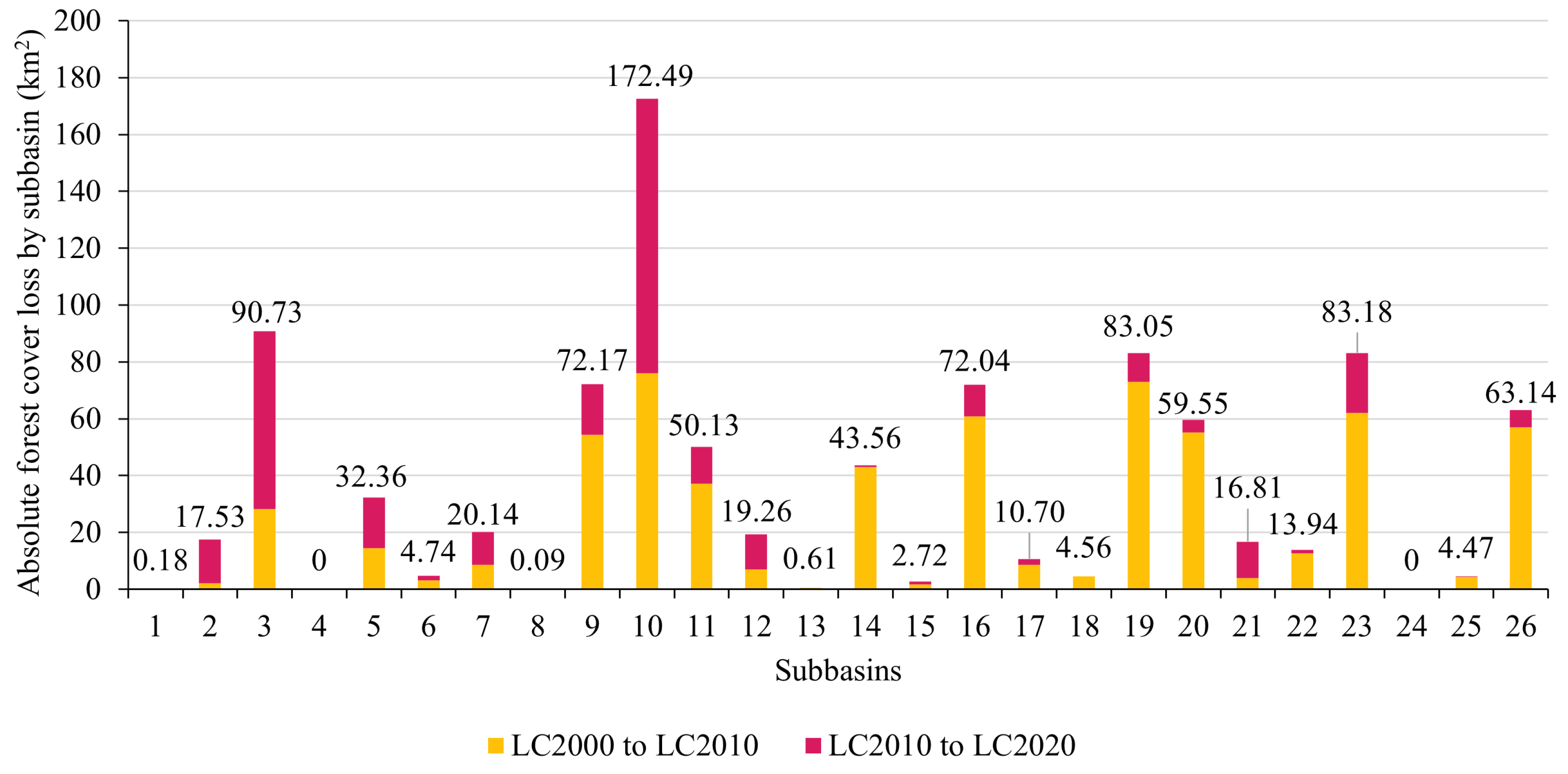
  • The sub-basin with the most absolute change in forest cover area from LC2000 to LC2020. This sub-basin was selected to identify the hydrological impacts of forest cover loss on the watershed region experiencing the most deforestation;
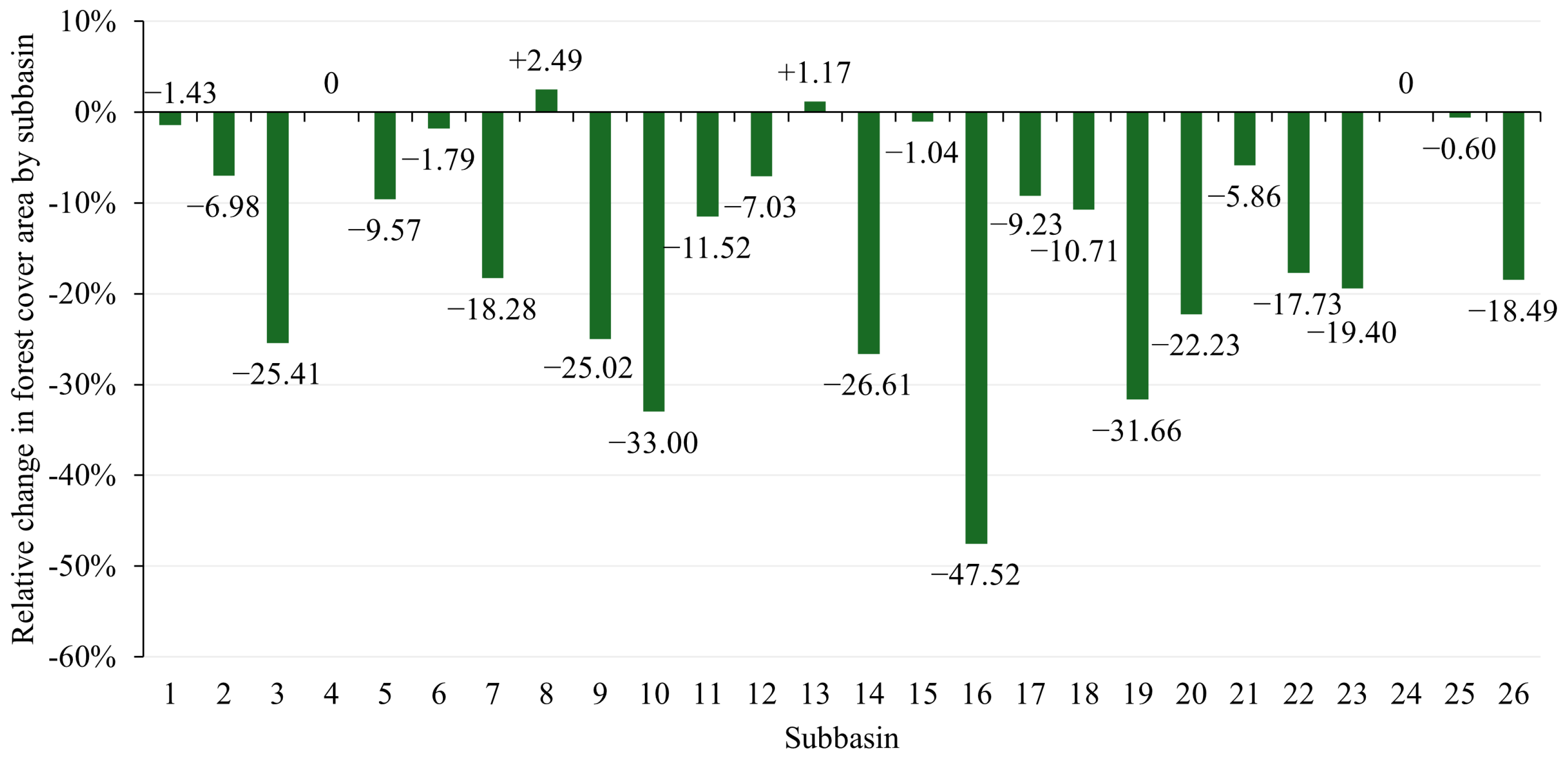
  • The sub-basin with the most relative change in forest cover area from LC2000 to LC2020. This sub-basin was selected to quantify the magnitude of localized hydrological impacts resulting from forest cover loss;
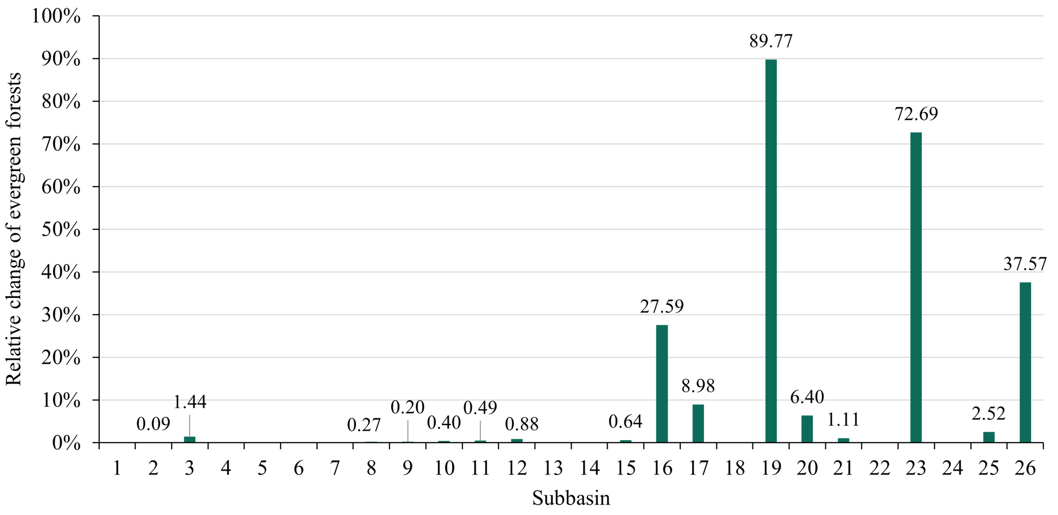
  • The sub-basin with the most relative change in forest cover areas from LC2020 to LC2020PA. This sub-basin was selected to understand the degree to which reforestation of agricultural encroachments in protected areas can alter local watershed hydrology.
The target hydrological dynamics for sub-basin analyses were water yield, sediment yield, surface runoff, ET, percolation, and base flow. Water yield is defined as the contribution of water to streamflow from surface runoff, baseflow, and lateral flow without pond abstractions [78], and this variable was used as a proxy for streamflow at the subwatershed level. Monthly period averages of each hydrological variable were calculated for each case study.

3. Results and Discussion

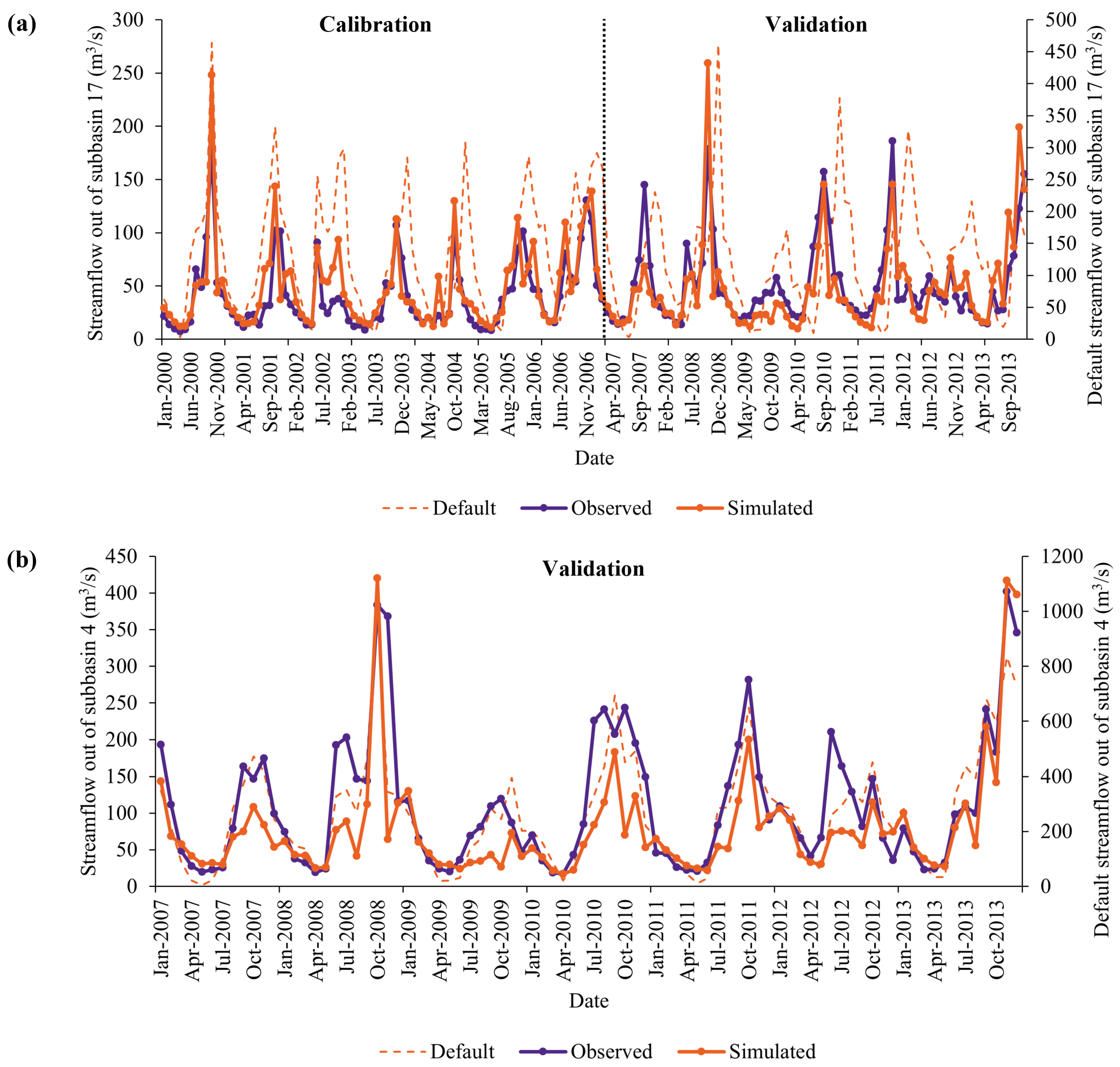
3.1. Model Performance and Evaluation

The SWAT model was calibrated on in situ streamflow from the BV gauge station (sub-basin 17). The calibration (2000 to 2006) was performed using daily average streamflow on the monthly time step. To calibrate the model, the chosen parameters were modified within their initial ranges using the iterative SPE algorithm until a satisfactory simulation was achieved in the fifth iteration. Table 6 shows the final ranges and fitted values for each chosen parameter.
The final sensitivity analysis is shown in Table 7. The most sensitive parameters in this study were, in order, SOL_K, GW_REVAP, and REVAPMN. These findings suggest that parameters controlling soil water, groundwater allocation, and ET are sensitive in the present model. Table 8 compares the parameter sensitivities of the current model to other SWAT models in subtropical and tropical watersheds. The parameters selected for calibration in this study have been determined as sensitive in other tropical and subtropical studies; however, the final sensitivity analysis of the present model differs from findings in previous studies. Other studies typically found CN2, which governs surface runoff, to be highly sensitive in tropical and subtropical watersheds.
In the present study, the inclusion of the somewhat uncommon cited ET parameter CANMX may have resulted in opposing parameter sensitivities typically observed in previous studies. During the calibration process, HRUs containing only evergreen forests were calibrated for CANMX based on findings from Jetten [86]. Jetten [86] determined that dry, evergreen forests in tropical Guyana intercepted around 17.3% of precipitation. Only HRUs covered by evergreen forests were selected for CANMX and CANMX depths in HRUs with other land cover types were not calibrated due to insufficient information about canopy storage and land cover class aggregation. The increase in CANMX in the calibrated model alters the water fluxes for soil water, groundwater, surface runoff, and ET; thereby, altering the interactions between model parameters dissimilarly to other models that do not incorporate CANMX.
SWAT model validation was performed using monthly in situ streamflow averages from BV and DR. Figure 6 compares the observed and simulated streamflow values from DR and BV during the calibration and validation periods. The monthly comparison between observed and simulated streamflow at BV shows satisfactory agreement between the in situ and modeled streamflows during calibration and validation. The monthly streamflow comparison at DR shows somewhat satisfactory agreement between the observed and simulated streamflow from 2007 to 2013. See Table 3 for the performance ratings used to evaluate the SWAT simulation in this study.
Table 9 presents the statistical results for R2, NSE, and PBIAS at BV and DR during the calibration and validation periods. At BV, the results for R2, NSE, and PBIAS were found satisfactory during the calibration and validation periods. For DR, R2 and NSE were satisfactory during validation. PBIAS was just below the satisfactory threshold from 2007 to 2013.
Calibration and validation were limited by the availability of in situ measurements. Streamflow data from the BV was unavailable from 2014 to 2020, limiting the duration of model calibration and validation during the study period. Direct measurements of other hydrological components like ET, groundwater fluxes, and surface runoff were also unavailable, requiring these processes to be inferred from available streamflow measurements. At the time of this study, in situ sediment concentrations were unavailable for incorporation into model calibration. Furthermore, integrating dam inflow and outflow data could improve the simulation accuracy of the present model. Reservoirs can alter downstream hydrological regimes and alter downstream flow patterns [87], and dam integration could reveal currently unaccounted streamflow regimes. Multi-gauge calibration is also recommended for larger watersheds. Using multiple gauges for calibration and validation would promote a more predictable streamflow uncertainty and capture more streamflow variation [88,89,90]. Previous research in Latin America demonstrated the potential for gathering time-series sediment concentration using satellite imagery [91,92,93]. These methods could be explored for their applicability in the BRW for calibration and validation.

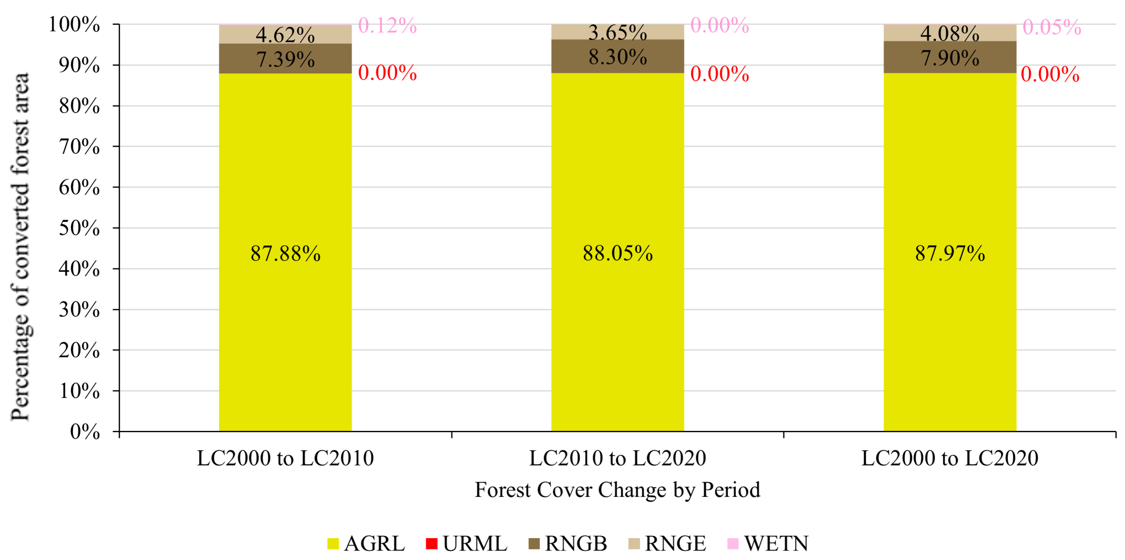
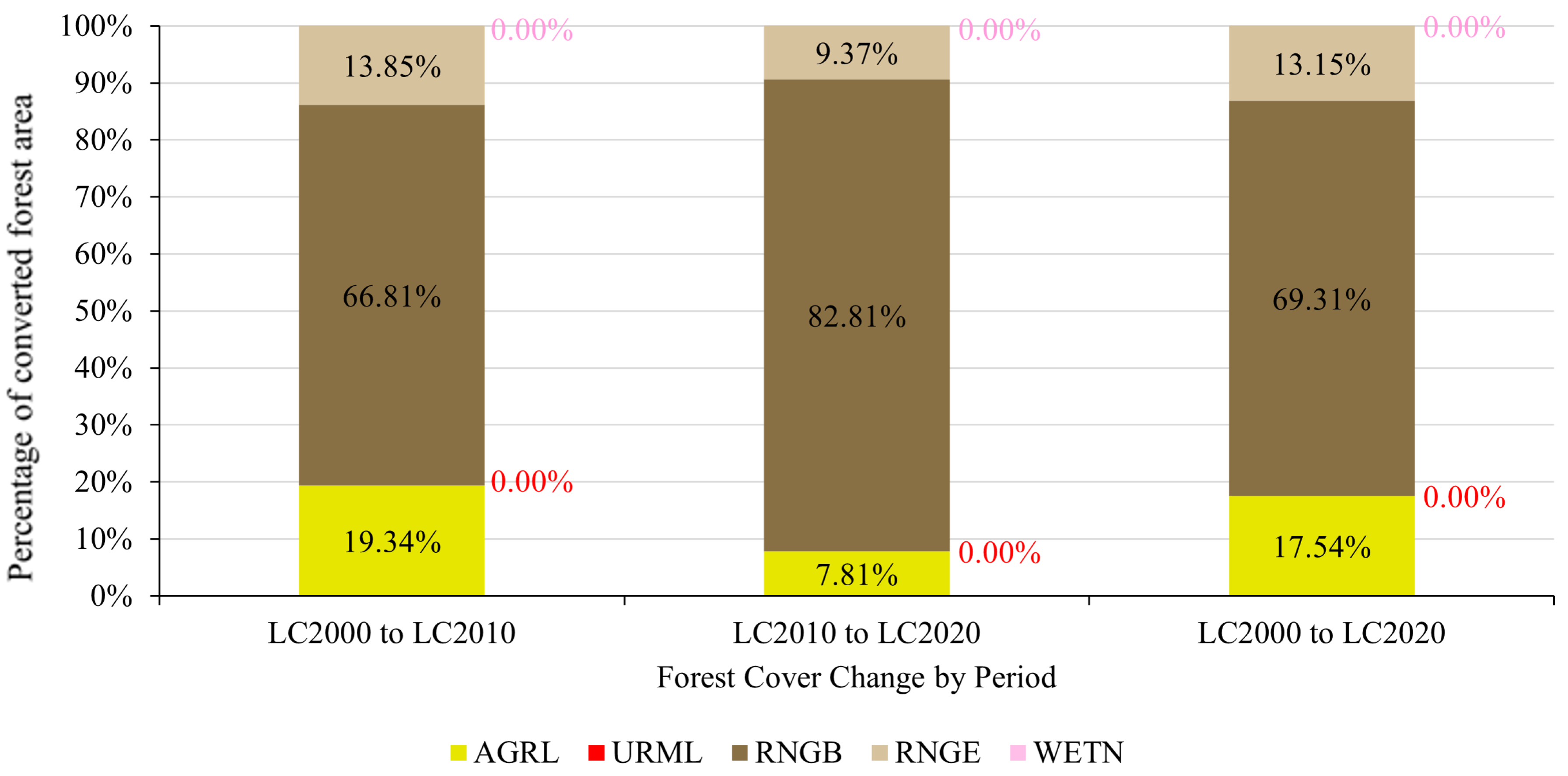
3.2. Trends in LULCC

3.2.1. Watershed-Level Trends

In this study, the total forest cover extent in the BRW declined from 71.38% (6240.60 km2) in 2000 to 60.65% (5302.44 km2) in 2020 Table 10. These figures translate to an absolute loss in forest cover area by 938.16 km2 and a relative decrease in forest cover area by 15.03% during the study period. The average forest cover loss rate from 2000 to 2020 was approximately 46.91 km2/yr. Temporally, the average rate of forest cover loss was higher from 2000 to 2010 (61.89 km2/yr) compared to 2010 to 2020 (31.92 km/yr). Agricultural expansion was identified in this study as the most predominant cause of forest cover replacement in the watershed from 2000 to 2020. Figure 7 shows that 66.79% (626.59 km2) of the total forest cover loss from 2000 to 2020 could be attributed to agricultural deforestation. The portion of forest cover lost due to agricultural expansion was greater from 2000 to 2010 (73.41%) compared to 2010 to 2020 (53.95%) (Figure 7). The second most prevalent LULCC contributing to forest cover loss in the BRW was forest degradation into shrublands. Figure 7 reveals that 28.40%, or 266.41 km2, of forest extent lost during the study period resulted from forest degradation into shrublands. The third most prevalent cause of forest cover loss was forest degradation into grassland, which consisted of 4.74%, or 44.50 km2, of total forest cover lost from 2000 to 2020. According to the results shown in Figure 7, forest conversion to urban areas or non-forested wetlands was relatively small during the study period. These findings corroborate with previous literature identifying agricultural expansion as a growing pressure on forested habitats and resources in the watershed [22,23,24,25,26,27,28]. Deforestation for agricultural purposes is common in the upper Guatemala reaches and middle reaches of the watershed [22,23,25]. Furthermore, denser populations in these regions put forests in these regions at higher risk of deforestation or degradation through logging, clear-cutting, and urban expansion [22]. LC2020PA was implemented to assess the influence of forest cover in these areas on watershed hydrological responses. Table 11 lists the portion of protected area extent converted to evergreen forests. Montañas Mayas Chiquibul was the protected area with the greatest increase in evergreen forest cover in LC2020PA. When applying this scenario, Table 10 shows that the total portion of BRW forest cover extent increased from 60.65% in LC2020 to 67.56% in LC2020PA. Significant portions of agricultural extent particularly in the upper Guatemalan regions of the watershed, were converted to evergreen cover. These findings provide implications for the effectiveness of protected areas in the region to safeguard against negative impacts on forest habitats from anthropogenic activities. The aggregation of ESA CCI land cover classes into simplified classes limited the representation of certain land covers in the study. All ESA CCI land cover classes representing croplands were aggregated, potentially leading to the overestimation of crop cover and the underrepresentation of forest cover. Furthermore, the coarser resolution of the ESA CCI global land cover may not capture smaller-scale land uses such as milpa cultivation. These are traditional intercropping systems encompassing an average area of 0.3 ha [94]. Pasturelands were also unclassified in the ESA CCI land cover dataset; therefore, pastures were indistinguishable from other land uses. Splitting agricultural classes into smaller crop or pasture classifications could be used to improve the present approach as seen in Astmann [95].

3.2.2. Case Study One: Sub-Basin with the Most Absolute Forest Change

Figure 8 depicts the absolute area of forest cover loss by sub-basin and reveals that sub-basin 10 experienced the most absolute forest cover loss of all sub-basins. From 2000 to 2020, Figure 8 shows that sub-basin 10 lost 172.49 km2 of forest cover from LULCCs. The rate of forest cover loss in sub-basin 10 increased from 7.59 km2/yr from 2000 to 2010 to 9.66 km2/yr from 2010 to 2020. Similar to the LULCC trends in the greater watershed, Figure 9 shows that agricultural expansion was the leading LULCC resulting in forest cover loss in sub-basin 10. About 87.97% of forest cover lost during the study period was caused by agricultural expansion (Figure 9).
Sub-basin 10 falls within the middle reaches of the watershed and this region is characterized by agricultural activities such as livestock farming and crop cultivation for sugarcane, grain, and citrus [22,28]. Furthermore, Spanish Lookout falls partially with sub-basin 10. Agricultural activities from this community contribute significantly to the Belizean economy; however, these activities also contribute to expansive land clearing and degradation [27,51]. The agricultural trends in sub-basin 10 identified in this study agree with previously discussed regional literature.

3.2.3. Case Study Two: Sub-Basin with the Most Relative Forest Change

Figure 10 shows the relative change in forest cover area by sub-basin from 2000 to 2020, and sub-basin 16 experienced the greatest relative change in forest cover of all sub-basins. The total area of forest cover in sub-basin 16 decreased from 152.28 km2 in 2000 to 79.92 km2 in 2020, constituting a nearly 50% relative decrease in forest area over the study period. The rate of forest cover loss decreased temporally from 6.14 km2/yr from 2000 to 2010 to 1.10 km2/yr from 2010 to 2020. Opposing the general LULCC trends previously identified, forest replacement with shrublands was identified as the leading cause of forest cover loss in sub-basin 16 (Figure 11). From 2000 to 2010, the portion of total replaced forest cover replaced by shrublands was 67% (Figure 11). This portion increased to 83% of forest cover losses from 2010 to 2020 (Figure 11).
Sub-basin 16 falls within the upper Belizean reaches of the BRW and contains a significant portion of the Mountain Pine Ridge Forest Reserve. This region faces a variety of natural and anthropogenic threats to local forests. Various studies and reports have reported increased tree mortality and disturbances in forest habitats resulting from beetle infestations [96,97,98,99]. Forest fires and hurricane damage may also provide potential natural causes of forest cover loss from degradation [100,101]. Previous studies also suggest that high road connectivity in the Mountain Pine Ridge Forest Reserve provides increased access to forest resources, which may put the region at higher risk for forest degradation [30,31]. The reported natural and anthropogenic activities may elucidate the drivers behind the LULCC trends observed in sub-basin 16.

3.2.4. Case Study Three: Sub-Basin with the Most Relative Forest Change in LC2020PA

Figure 12 depicts the relative change in LC2020 forest cover area when implementing LC2020PA by each sub-basin. Sub-basin 19 was the sub-basin with the largest relative change in forest cover in this scenario, increasing relatively by 89.77% from 2000 to 2020. The extent of evergreen forests increased from 49.87% of the sub-basin’s total area in LC2020 to 94.63% in LC2020PA. Reforestation of the [protected area] is behind the increase in forest cover area in the sub-basin. This sub-basin falls within the upper Guatemalan reaches of the watershed, which is characterized by high agricultural activity and denser populations than downstream reaches. Encroachment into protected areas in this region for agriculture and resource provision has been reported in this region [22,25].

3.3. Hydrological Responses to LULCC

3.3.1. Watershed-Level Responses

To isolate the impacts of LULCCs from the impacts of precipitation variation on hydrological response, the period averages (2000 to 2020) were calculated and compared for each land cover scenario. Table 12 depicts the relative changes in monthly averages of hydrological components for the watershed. This study found that the average monthly streamflow out of the BRW increased by 16.86% from 2000 to 2020 Table 12. Temporally, the average monthly streamflow experienced a greater relative change (12.22%) from 2000 to 2010 compared to the change (4.14%) from 2010 to 2020. This change is likely influenced by the larger rate of forest cover loss from 2000 to 2010 compared to 2010 to 2020. When implementing LC2020PA, the average monthly streamflow from LC2020 decreased by 11.67%. If agricultural lands were replaced by evergreen forests in 2020, the mean average streamflow would increase by 3.23% from 2000 to 2020. Therefore, the addition of evergreen forests within protected areas would mitigate some of the change in streamflow that has been experienced by the watershed. Table 12 shows that the components with the greatest relative change in their hydrological responses were sediment yield (+34.40%) and surface runoff (+24.95%). The components that had the least relative change over the study period were ET (−3.52%) and percolation (+3.40%). When the LC2020 is replaced by LC2020PA, sediment yield, and surface runoff have the greatest relative changes between the actual and alternative scenarios. ET and percolation in the watershed had the smallest relative change when the scenario was implemented by +2.32% and −0.77%, respectively.
Based on previous literature, groundwater recharge, to which percolation contributes significantly, is expected to decrease in deforested regions [11,12]. The hydrological response of percolation in this study opposed the expected response. Overestimation of CANMX by evergreen forests may have led to the underestimation of percolation in forested HRUs. More precipitation is intercepted by the forest canopy and less precipitation falls to the ground when CANMX is large; therefore, the model simulates less water infiltrating the soil and percolating through the subsurface. To combat this limitation, a lower CANMX could be selected in the default model for future models. Increases in streamflow corroborate with findings from previous SWAT studies in tropical and subtropical catchments that found that streamflow increased due to deforestation and agricultural expansion [34,36,40,46]. Moreover, studies of Belizean watersheds using empirical hydrological models to investigate LULCC impacts have suggested that surface runoff will increase due to deforestation and agricultural expansion [24,32]. Forest degradation and removal have led to increased erosion and reduced water quality in the BRW [22], and the current study has found that regions experiencing increased forest cover loss have also experienced increased runoff and sediment yields. However, the magnitude of the change in sediment yield could not be validated due the current unavailability of in situ sediment measurements. Results from this study suggest that the infiltration capacity of the BRW has been negatively impacted by LULCC. Reforestation in protected areas has potential to mitigate some of the hydrological changes experienced in the watershed by reducing water and sediment yields. The reforestation of agricultural areas scenario primarily affected Guatemalan protected areas in the steeper, upper reaches of the watershed. Land management changes in headwater catchments influence the accumulation of upper watershed streamflow and the transportation of fine sediments downstream [102]. This finding highlights the importance of forest cover in the watershed’s upper reaches for regulating downstream flow regimes and sediment transport. Various studies have indicated that reforestation and habitat restoration activities in upper watersheds help mitigate runoff and associated eroded sediments [103,104,105].

3.3.2. Case Study Responses

Sub-basin case studies were used to understand how land cover trends in the BRW have impacted hydrological responses at smaller scales. Sub-basin 10 was identified as the sub-basin with the largest absolute loss of forest extent in the watershed, primarily caused by agricultural expansion. Sediment yield was the hydrological component with the largest relative change (+354.73%) from 2000 to 2020 (Table 13). Water yield, the proxy for streamflow, increased by 65.70% due to LULCCs experienced in the sub-basin during the study period (Table 13). Surface runoff and baseflow also experienced substantial increases from 2000 to 2020. The relative percentage of percolation increases during this period as well, which may be attributed to loss of forest cover. Their removal likely causes less water to be removed via ET, leading to increased percolation. Furthermore, the composition of the soils of this sub-basin is dominated by humic nitisols which have low runoff potential.
Sub-basin 16 represents the sub-basin with the greatest relative change in forest cover extent due to LULCCs over the study period. The predominant vehicle of forest cover loss in the sub-basin was forest degradation into shrublands. Monthly average water yield in the sub-basin increased by 44.36% due to the LULCCs experienced over the study period (Table 14). Of the hydrological components, monthly average sediment yield experienced the greatest relative change (+537.84%) (Table 14). Baseflow and surface runoff also experienced significant increases. Percolation had the smallest relative change at +3.40%.
Sub-basin 19 represents the sub-basin with the greatest relative change in forest extent when replacing LC2020 with LC2020PA. The exploration of hydrological response changes in this sub-basin elucidated the impact of increased forest cover on watershed hydrology. In addition, this scenario highlighted the role of maintaining protected area forests in mitigating runoff and sediment-generating soil erosion in response to excessive precipitation. Sediment yield experienced the greatest relative change compared to the other modeled variables, decreasing by −99.18% from LC2020 when compared to the alternative land cover scenario (LC2020PA), falling from 29.29 tons/km2 annually to 0.24 tons/km2 annually (Table 15). Surface runoff and water yield experienced significant relative decreases due to increasing forest cover in the sub-basin. In LC2020PA, ET had the greatest relative change amongst the case studies, increasing by 17.74% compared to LC2020 (Table 15).
Increases in surface runoff depths are enhanced at the local scale from forest cover loss. Reduction in ET was greater locally due to larger concentrations of deforestation and degradation. Greater reductions in ET are correlated with greater losses of groundwater to baseflow in sub-basins experiencing forest cover loss. Decreased demands for soil water and less interception may influence this pattern from due to lessening forest cover. Furthermore, tropical deforestation may reduce local precipitation and lead to drier local climates [106], providing implications for water availability in the region.

4. Conclusions

This study assessed the impact of LULCC on the hydrological dynamics of the BRW from 2000 to 2020 using ArcSWAT. ESA CCI datasets were used to determine LULCCs in the watershed, and these were combined with soil, elevation, meteorological data, and ancillary datasets for protected areas, stream networks, water bodies, and river stages to build the BRW SWAT model. The predominant LULCC leading to the depletion of forest cover in the BRW was agricultural expansion, which was attributed to 66.79%, or 626.59 km2, of total forest cover loss during the study period. The decrease in forest cover extent from 71.38% in 2000 to 60.65% in 2020 was primarily caused by agricultural growth in the middle and upper reaches of the BRW. Agricultural expansion in Belize primarily occurred outside designated protected areas while protected areas in Guatemala were more likely to contain agricultural encroachment. Due to LULCCs in the BRW, findings from this study suggest that monthly average streamflow has increased by 16.86% from LC2000 to LC2020. Other alterations in monthly average hydrological responses found during the period were a 34.40% increase in sediment yield, a 24.95% increase in surface runoff, a 16.02% increase in water yield, an 11.58% increase in baseflow, a 3.40% increase in percolation, and a 3.52% decrease in ET. These results suggest that LULCCs in the BRW have decreased the ability of the watershed to retain water as soil moisture and groundwater recharge. When applying LC2020PA, streamflow was found to decrease by 11.67% compared to LC2020 and increase by 3.23% compared to LC2000. These findings suggest the importance of maintaining forests in protected areas to mitigate hydrological impacts from LULCCs. Generally, the methodology and results of this study present a foundation for LULCC analyses using hydrological modeling in data-scarce regions. Data gaps in meteorological measurements provided a challenge for model development; however, this was mitigated through the use of long-term period averages in SWAT’s WGEN. However, data gaps in streamflow measurements at in situ gauge stations limited the calibration and validation processes. Exploration of modeled streamflow measurements from initiatives such as the Group on Earth Observations Global Water Sustainability (GEOGLOWS) could provide a useful resource for mitigating streamflow data gaps and improving the accuracy of model calibration and validation [107]. Future studies in the region could build upon the foundation outlined in this study by implementing multi-variable and multi-gauge calibration and validation. Moreover, the evaluation of the other hydrological components presented here could refine the accuracy of the model and improve the understanding of the impacts of LULCCs on water resources in the region.

Author Contributions

Conceptualization, N.K.L.C., R.E.G., B.E.H.S. and E.A.C.; methodology, N.K.L.C., R.E.G., B.E.H.S., E.A.C. and C.D.; software, N.K.L.C.; validation, N.K.L.C.; formal analysis, N.K.L.C.; investigation, N.K.L.C.; resources, N.K.L.C., R.E.G., B.E.H.S., E.A.C., C.D. and T.H.; data curation, N.K.L.C.; writing—original draft preparation, N.K.L.C.; writing—review and editing, R.E.G., B.E.H.S., E.A.C., C.D. and T.H.; visualization, N.K.L.C.; supervision, R.E.G., B.E.H.S., E.A.C. and C.D.; project administration, R.E.G., B.E.H.S. and E.A.C.; funding acquisition, R.E.G. All authors have read and agreed to the published version of the manuscript.

Funding

This research was funded by NASA Cooperative Agreement (SERVIR) grant number 80MSFC22N0004.

Data Availability Statement

Elevation data were obtained from the Shuttle Radar Topography Mission (SRTM) using the United States Geological Survey (USGS) EarthExplorer (https://earthexplorer.usgs.gov/ (accessed on 8 June 2023)). Soil data were obtained from the Harmonized World Soil Database (HWSD) Ver 1.2 (www.fao.org/soils-portal/data-hub/soil-maps-and-databases/harmonized-world-soil-database-v12/en/ (accessed on 12 July 2023)). Land cover data were obtained from the European Space Agency’s (ESA) Climate Change Initiative (CCI) (https://cds.climate.copernicus.eu/datasets/satellite-land-cover?tab=overview (accessed on 9 June 2023)). Protected areas data were obtained from Protected Planet (https://www.protectedplanet.net/en (accessed on 24 January 2024)). Meteorological data for Belizean weather stations were requested from the National Meteorological Service of Belize (NMSB) (https://nms.gov.bz/ (accessed on 15 June 2023)). Additional precipitation and temperature data were obtained for Climate Hazards Group Infrared Precipitation with Stations (CHIRPS) and Climate Hazards Group Infrared Temperature with Stations (CHIRTS-daily) from the Soil and Water Assessment Tool (SWAT) website (https://swat.tamu.edu/software/ (accessed on 12 November 2023)). Solar radiation and wind speed data were obtained for the National Renewable Energy Laboratory’s (NREL) Physical Solar Model Ver 3 from the National Solar Radiation Database (NSRDB) (https://nsrdb.nrel.gov/data-viewer (accessed on 18 June 2024)). Belizean water body data were obtained from the Biodiversity and Environmental Resource Data System of Belize (BERDS) (https://datacatalog.worldbank.org/search/dataset/0040692 (accessed on 18 July 2024)). Guatemalan water body data were obtained from the World Bank Data Catalog (https://datacatalog.worldbank.org/search/dataset/0040692 (accessed on 18 July 2024)). Stream network and watershed boundary data were provided by SERVIR. In situ streamflow and stage measurements from the Belize River Watershed (BRW) were provided by the National Hydrological Service of Belize (NHSB). Data created during the present study are available on Zenodo (https://zenodo.org/records/15361440 (accessed on 7 May 2025)).

Acknowledgments

Authors wish to acknowledge Sundar Christopher of the University of Alabama in Huntsville for his supervision and direction. We wish to express sincere gratitude to the NHSB for providing hydrological data and providing local insights about the study area. Authors also wish to thank the NMSB for providing meteorological data for model development. We wish to give thanks to the SERVIR Science Coordination Office (principally Dan Irwin, Ashutosh Limaye, and Eric Anderson) for facilitating this research and providing methodological/conceptual support. Authors are thankful to all editors and reviewers who helped improve this manuscript.

Conflicts of Interest

The authors declare no conflicts of interest.

Abbreviations

The following abbreviations are used in this manuscript:
LULCCLand use and land cover change
ETEvapotranspiration
SWATSoil and Water Assessment Tool
BRWBelize River Watershed
N-SPECTNon-Point Source Pollution and Erosion Comparison Tool
HRUHydrological response unit
PSOParticle SWAT Organization
SPESWAT Parameter Estimator
SUFI-2SWAT-CUP Sequential Uncertainty Fitting
95PPU95% Confidence Interval
DEMDigital elevation model
SRTMShuttle Radar Topography Mission
USGSUnited States Geological Survey
HWSDHarmonized World Soil Database
FAOFood and Agriculture Organization of the United Nations
ESAEuropean Space Agency
CCIClimate Change Initiative
NMSBNational Meteorological Service of Belize
CHIRPSClimate Hazards Group Infrared Precipitation with Stations
CHIRTS-dailyClimate Hazards Group Infrared Temperature with Stations
NSRDBNational Solar Radiation Database
WGENSWAT Weather Generator
DRDouble Run
BVBenque Viejo
NHSBNational Hydrological Service of Belize
BERDSBiodiversity and Environmental Resource Data System of Belize
PETPotential evapotranspiration
R 2 Coefficient of determination
N S E Nash–Sutcliffe efficiency
P B I A S Percent bias
GEOGLOWS Group on Earth Observations Global Water Sustainability

References

  1. Garg, V.; Nikam, B.R.; Thakur, P.K.; Aggarwal, S.P.; Gupta, P.K.; Srivastav, S.K. Human-Induced Land Use Land Cover Change and Its Impact on Hydrology. HydroResearch 2019, 1, 48–56. [Google Scholar] [CrossRef]
  2. Hassan, Z.; Shabbir, R.; Ahmad, S.S.; Malik, A.H.; Aziz, N.; Butt, A.; Erum, S. Dynamics of Land Use and Land Cover Change (LULCC) Using Geospatial Techniques: A Case Study of Islamabad Pakistan. SpringerPlus 2016, 5, 812. [Google Scholar] [CrossRef] [PubMed]
  3. Lambin, E.F.; Turner, B.L.; Geist, H.J.; Agbola, S.B.; Angelsen, A.; Bruce, J.W.; Coomes, O.T.; Dirzo, R.; Fischer, G.; Folke, C.; et al. The Causes of Land-Use and Land-Cover Change: Moving Beyond the Myths. Glob. Environ. Change 2001, 11, 261–269. [Google Scholar] [CrossRef]
  4. Curtis, P.G.; Slay, C.M.; Harris, N.L.; Tyukavina, A.; Hansen, M.C. Classifying Drivers of Global Forest Loss. Science 2018, 361, 1108–1111. [Google Scholar] [CrossRef]
  5. Kroeger, T.; Klemz, C.; Boucher, T.; Fisher, J.R.B.; Acosta, E.; Cavassani, A.T.; Dennedy-Frank, P.J.; Garbossa, L.; Blainski, E.; Santos, R.C.; et al. Returns on Investment in Watershed Conservation: Application of a Best Practices Analytical Framework to the Rio Camboriú Water Producer Program, Santa Catarina, Brazil. Sci. Total Environ. 2019, 657, 1368–1381. [Google Scholar] [CrossRef]
  6. de Mello, K.; Taniwaki, R.H.; de Paula, F.R.; Valente, R.A.; Randhir, T.O.; Macedo, D.R.; Leal, C.G.; Rodrigues, C.B.; Hughes, R.M. Multiscale Land Use Impacts on Water Quality: Assessment, Planning, and Future Perspectives in Brazil. J. Environ. Manag. 2020, 270, 110879. [Google Scholar] [CrossRef]
  7. Taffarello, D.; Srinivasan, R.; Mohor, G.S.; Guimarães, J.L.B.; do Carmo Calijuri, M.; Mendiondo, E.M. Modeling Freshwater Quality Scenarios with Ecosystem-Based Adaptation in the Headwaters of the Cantareira System, Brazil. Hydrol. Earth Syst. Sci. 2018, 22, 4699–4723. [Google Scholar] [CrossRef]
  8. Anache, J.A.A.; Wendland, E.C.; Oliveira, P.T.S.; Flanagan, D.C.; Nearing, M.A. Runoff and Soil Erosion Plot-Scale Studies under Natural Rainfall: A Meta-Analysis of the Brazilian Experience. Catena 2017, 152, 29–39. [Google Scholar] [CrossRef]
  9. Bruijnzeel, L.A. Hydrological Functions of Tropical Forests: Not Seeing the Soil for the Trees? Agric. Ecosyst. Environ. 2004, 104, 185–228. [Google Scholar] [CrossRef]
  10. Costanza, R.; d’Arge, R.; de Groot, R.; Farber, S.; Grasso, M.; Hannon, B.; Limburg, K.; Naeem, S.; O’Neill, R.V.; Paruelo, J.; et al. The Value of the World’s Ecosystem Services and Natural Capital. Nature 1997, 387, 253–260. [Google Scholar] [CrossRef]
  11. Esen, S.E.; Hein, L.; Cuceloglu, G. Accounting for the Water Related Ecosystem Services of Forests in the Southern Aegean Region of Turkey. Ecol. Indic. 2023, 154, 110553. [Google Scholar] [CrossRef]
  12. Krishnaswamy, J.; Bonell, M.; Venkatesh, B.; Purandara, B.K.; Rakesh, K.N.; Lele, S.; Kiran, M.C.; Reddy, V.; Badiger, S. The Groundwater Recharge Response and Hydrologic Services of Tropical Humid Forest Ecosystems to Use and Reforestation: Support for the “Infiltration-Evapotranspiration Trade-off Hypothesis”. J. Hydrol. 2013, 498, 191–209. [Google Scholar] [CrossRef]
  13. Brookhuis, B.J.; Hein, L.G. The Value of the Flood Control Service of Tropical Forests: A Case Study for Trinidad. For. Policy Econ. 2016, 62, 118–124. [Google Scholar] [CrossRef]
  14. Menéndez, P.; Losada, I.J.; Torres-Ortega, S.; Narayan, S.; Beck, M.W. The Global Flood Protection Benefits of Mangroves. Sci. Rep. 2020, 10, 4404. [Google Scholar] [CrossRef]
  15. Gordon, L.J.; Steffen, W.; Jönsson, B.F.; Folke, C.; Falkenmark, M.; Johannessen, Å. Human Modification of Global Water Vapor Flows from the Land Surface. Proc. Natl. Acad. Sci. USA 2005, 102, 7612–7617. [Google Scholar] [CrossRef]
  16. Scanlon, B.R.; Jolly, I.; Sophocleous, M.; Zhang, L. Global Impacts of Conversions from Natural to Agricultural Ecosystems on Water Resources: Quantity versus Quality. Water Resour. Res. 2007, 43, W03437. [Google Scholar] [CrossRef]
  17. Akinnawo, S.O. Eutrophication: Causes, Consequences, Physical, Chemical and Biological Techniques for Mitigation Strategies. Environ. Chall. 2023, 12, 100733. [Google Scholar] [CrossRef]
  18. Owens, P.N. Soil Erosion and Sediment Dynamics in the Anthropocene: A Review of Human Impacts during a Period of Rapid Global Environmental Change. J. Soils Sediments 2020, 20, 4115–4143. [Google Scholar] [CrossRef]
  19. Rápalo, L.M.C.; Uliana, E.M.; Moreira, M.C.; da Silva, D.D.; de Melo Ribeiro, C.B.; da Cruz, I.F.; dos Reis Pereira, D. Effects of Land-Use and -Cover Changes on Streamflow Regime in the Brazilian Savannah. J. Hydrol. Reg. Stud. 2021, 38, 100934. [Google Scholar] [CrossRef]
  20. Sadhwani, K.; Eldho, T.I.; Jha, M.K.; Karmakar, S. Effects of Dynamic Land Use/Land Cover Change on Flow and Sediment Yield in a Monsoon-Dominated Tropical Watershed. Water 2022, 14, 3666. [Google Scholar] [CrossRef]
  21. Ware, H.H.; Chang, S.W.; Lee, J.E.; Chung, I.-M. Assessment of Hydrological Responses to Land Use and Land Cover Changes in Forest-Dominated Watershed Using SWAT Model. Water 2024, 16, 528. [Google Scholar] [CrossRef]
  22. Carrias, A.; Cano, A.; Saqui, P.; Ake, J.; Boles, E. Management Plan for the Belize River Watershed; University of Belize: Belmopan, Belize, 2018; pp. 1–197. [Google Scholar]
  23. Bridgewater, S. A Natural History of Belize: Inside the Maya Forest, 1st ed.; University of Texas Press: Austin, TX, USA, 2012; pp. 1–400. [Google Scholar]
  24. Cherrington, E.A.; Kay, E.; Waight-Cho, I. Modelling the Impacts of Climate Change and Land Use Change on Belize’s Water Resources: Potential Effects on Erosion and Runoff. Technical Report; University of Belize: Belmopan, Belize, 2015; pp. 1–32. [Google Scholar] [CrossRef]
  25. Chicas, S.D.; Omine, K.; Arevalo, B.; Ford, J.B.; Sugimura, K. Deforestation Along the Maya Mountain Massif Belize-Guatemala Border. Int. Arch. Photogramm. Remote Sens. Spat. Inf. Sci. 2016, 41, 597–602. [Google Scholar] [CrossRef]
  26. Coe, M.R. Landscape Effects on Soil Fertility Across Belize. Master’s Thesis, Montana State University, Bozeman, MT, USA, 2022. [Google Scholar]
  27. Di Fiore, S. Remote Sensing and Exploratory Data Analysis as Tools to Rapidly Evaluate Forest Cover Change and Set Conservation Priorities Along the Belize River, Belize. Master’s Thesis, Columbia University, New York, NY, USA, 2002. [Google Scholar]
  28. Young, C.A. Belize’s Ecosystems: Threats and Challenges to Conservation in Belize. Trop. Conserv. Sci. 2008, 1, 18–33. [Google Scholar] [CrossRef]
  29. Astmann, B.; Hobbs, S.R.; Martin, P. Monitoring and Modeling Glyphosate Transport in the Belize River Watershed. In Proceedings of the 2020 IEEE Global Humanitarian Technology Conference (GHTC), Virtual, 29 October–1 November 2020; pp. 1–8. [Google Scholar]
  30. Folkard-Tapp, H. Deforestation in Belize-What, Where and Why. bioRxiv 2020, 1–43. [Google Scholar] [CrossRef]
  31. Wyman, M.S.; Stein, T.V. Modeling Social and Land-Use/Land-Cover Change Data to Assess Drivers of Smallholder Deforestation in Belize. Appl. Geogr. 2010, 30, 329–342. [Google Scholar] [CrossRef]
  32. Martín-Arias, V.; Evans, C.; Griffin, R.; Cherrington, E.A.; Lee, C.M.; Mishra, D.R.; Gomez, N.A.; Rosado, A.; Callejas, I.A.; Jay, J.A.; et al. Modeled Impacts of LULC and Climate Change Predictions on the Hydrologic Regime in Belize. Front. Environ. Sci. 2022, 10, 848085. [Google Scholar] [CrossRef]
  33. Chen, Y.; Xu, C.-Y.; Chen, X.; Xu, Y.; Yin, Y.; Gao, L.; Liu, M. Uncertainty in Simulation of Land-Use Change Impacts on Catchment Runoff with Multi-Timescales Based on the Comparison of the HSPF and SWAT Models. J. Hydrol. 2019, 573, 486–500. [Google Scholar] [CrossRef]
  34. de Oliveira Serrão, E.A.; Silva, M.T.; Ferreira, T.R.; Paiva de Ataide, L.C.; Assis dos Santos, C.; Meiguins de Lima, A.M.; de Paulo Rodrigues da Silva, V.; de Assis Salviano de Sousa, F.; Cardoso Gomes, D.J. Impacts of Land Use and Land Cover Changes on Hydrological Processes and Sediment Yield Determined Using the SWAT Model. Int. J. Sediment Res. 2022, 37, 54–69. [Google Scholar] [CrossRef]
  35. Khalid, K.; Ali, M.F.; Rahman, N.F.A.; Mispan, M.R.; Haron, S.H.; Othman, Z.; Bachok, M.F. Sensitivity Analysis in Watershed Model Using SUFI-2 Algorithm. Procedia Eng. 2016, 162, 441–447. [Google Scholar] [CrossRef]
  36. Khorn, N.; Ismail, M.H.; Nurhidayu, S.; Kamarudin, N.; Sulaiman, M.S. Land Use/Land Cover Changes and Its Impact on Runoff Using SWAT Model in the Upper Prek Thnot Watershed in Cambodia. Environ. Earth Sci. 2022, 81, 466. [Google Scholar] [CrossRef]
  37. Lin, B.; Chen, X.; Yao, H. Threshold of Sub-Watersheds for SWAT to Simulate Hillslope Sediment Generation and Its Spatial Variations. Ecol. Indic. 2020, 111, 106040. [Google Scholar] [CrossRef]
  38. Lucas-Borja, M.E.; Carrà, B.G.; Nunes, J.P.; Bernard-Jannin, L.; Zema, D.A.; Zimbone, S.M. Impacts of Land-Use and Climate Changes on Surface Runoff in a Tropical Forest Watershed (Brazil). Hydrol. Sci. J. 2020, 65, 1956–1973. [Google Scholar] [CrossRef]
  39. Marhaento, H.; Booij, M.J.; Rientjes, T.H.M.; Hoekstra, A.Y. Attribution of Changes in the Water Balance of a Tropical Catchment to Land Use Change Using the SWAT Model. Hydrol. Process. 2017, 31, 2029–2040. [Google Scholar] [CrossRef]
  40. McGinn, A.J.; Wagner, P.D.; Htike, H.; Kyu, K.K.; Fohrer, N. Twenty Years of Change: Land and Water Resources in the Chindwin Catchment, Myanmar between 1999 and 2019. Sci. Total Environ. 2021, 798, 148766. [Google Scholar] [CrossRef] [PubMed]
  41. Moreira, L.L.; Schwamback, D.; Rigo, D. Sensitivity Analysis of the Soil and Water Assessment Tools (SWAT) Model in Streamflow Modeling in a Rural River Basin. Rev. Ambient. Água 2018, 13, e2221. [Google Scholar] [CrossRef]
  42. Nguyen, T.V.; Dietrich, J.; Dang, T.D.; Tran, D.A.; Van Doan, B.; Sarrazin, F.J.; Abbaspour, K.; Srinivasan, R. An Interactive Graphical Interface Tool for Parameter Calibration, Sensitivity Analysis, Uncertainty Analysis, and Visualization for the Soil and Water Assessment Tool. Environ. Model. Softw. 2022, 156, 105497. [Google Scholar] [CrossRef]
  43. Oo, H.T.; Zin, W.W.; Kyi, C.C.T. Analysis of Streamflow Response to Changing Climate Conditions Using SWAT Model. Civ. Eng. J. 2020, 6, 194–209. [Google Scholar] [CrossRef]
  44. Sinha, R.K.; Eldho, T.I. Effects of Historical and Projected Land Use/Cover Change on Runoff and Sediment Yield in the Netravati River Basin, Western Ghats, India. Environ. Earth Sci. 2018, 77, 111. [Google Scholar] [CrossRef]
  45. Wagner, P.D.; Kumar, S.; Schneider, K. An Assessment of Land Use Change Impacts on the Water Resources of the Mula and Mutha Rivers Catchment Upstream of Pune, India. Hydrol. Earth Syst. Sci. 2013, 17, 2233–2246. [Google Scholar] [CrossRef]
  46. Yan, B.; Fang, N.F.; Zhang, P.C.; Shi, Z.H. Impacts of Land Use Change on Watershed Streamflow and Sediment Yield: An Assessment Using Hydrologic Modelling and Partial Least Squares Regression. J. Hydrol. 2013, 484, 26–37. [Google Scholar] [CrossRef]
  47. Zhang, H.; Wang, B.; Liu, D.L.; Zhang, M.; Leslie, L.M.; Yu, Q. Using an Improved SWAT Model to Simulate Hydrological Responses to Land Use Change: A Case Study of a Catchment in Tropical Australia. J. Hydrol. 2020, 585, 124822. [Google Scholar] [CrossRef]
  48. Felgate, S.L.; Barry, C.D.G.; Mayor, D.J.; Sanders, R.; Carrias, A.; Young, A.; Fitch, A.; Mayorga-Adame, C.G.; Andrews, G.; Brittain, H.; et al. Conversion of Forest to Agriculture Increases Colored Dissolved Organic Matter in a Subtropical Catchment and Adjacent Coastal Environment. J. Geophys. Res. Biogeo. 2021, 126, e2021JG006295. [Google Scholar] [CrossRef]
  49. Ramsar Sites Information Service: Parque Nacional Yaxhá-Nakum-Naranjo. Available online: https://rsis.ramsar.org/ris/1599 (accessed on 27 November 2024).
  50. Annual Report: 2018–2019; Statistical Institute of Belize: Belmopan, Belize, 2019; pp. 1–44. Available online: www.sib.org.bz (accessed on 24 July 2023).
  51. Belize’s Fifth National Report to the Convention on Biological Diversity; Ministry of Forestry, Fisheries and Sustainable Development: Belmopan, Belize, 2014; pp. 1–141.
  52. Atlas Centroamericano para la Gestión Sostenible del Territorio; Comisión Centroamericana de Ambiente y Desarrollo (CCAD): San Salvador, El Salvador, 2011; pp. 1–162.
  53. FAO Soils Portal: Harmonized World Soil Database v 1.2. Available online: www.fao.org/soils-portal/data-hub/soil-maps-and-databases/harmonized-world-soil-database-v12/en/ (accessed on 12 July 2023).
  54. Gassman, P.W.; Reyes, M.R.; Green, C.H.; Arnold, J.G. The Soil and Water Assessment Tool: Historical Development, Applications, and Future Research Directions. Trans. ASABE 2007, 50, 1211–1250. [Google Scholar] [CrossRef]
  55. Li, D.; Qu, S.; Shi, P.; Chen, X.; Xue, F.; Gou, J.; Zhang, W. Development and Integration of Sub-Daily Flood Modelling Capability within the SWAT Model and a Comparison with XAJ Model. Water 2018, 10, 1263. [Google Scholar] [CrossRef]
  56. Maharjan, G.R.; Park, Y.S.; Kim, N.W.; Shin, D.S.; Choi, J.W.; Hyun, G.W.; Jeon, J.-H.; Ok, Y.S.; Lim, K.J. Evaluation of SWAT Sub-Daily Runoff Estimation at Small Agricultural Watershed in Korea. Front. Environ. Sci. Eng. 2013, 7, 109–119. [Google Scholar] [CrossRef]
  57. Yang, X.; Liu, Q.; He, Y.; Luo, X.; Zhang, X. Comparison of Daily and Sub-Daily SWAT Models for Daily Streamflow Simulation in the Upper Huai River Basin of China. Stoch. Environ. Res. Risk Assess 2016, 30, 959–972. [Google Scholar] [CrossRef]
  58. Moriasi, D.N.; Arnold, J.G.; Van Liew, M.W.; Bingner, R.L.; Harmel, R.D.; Veith, T.L. Model Evaluation Guidelines for Systematic Quantification of Accuracy in Watershed Simulations. Trans. ASABE 2007, 50, 885–900. [Google Scholar] [CrossRef]
  59. Abbaspour, K.C. User Manual for SWATCUP-2019/SWATCUP-Premium/SWATplusCUP Calibration and Uncertainty Analysis Programs; 2w2e Consulting GmbH Publication: Duebendorf, Switzerland, 2022; pp. 1–68. [Google Scholar]
  60. Abbaspour, K.C. SWAT Calibration and Uncertainty Programs—A User Manual; Eawag: Duebendorf, Switzerland, 2015; pp. 1–100. [Google Scholar]
  61. USGS EarthExplorer. Available online: https://earthexplorer.usgs.gov/ (accessed on 8 June 2023).
  62. Stehr, A.; Aguayo, M.; Link, O.; Parra, O.; Romero, F.; Alcayaga, H. Modelling the Hydrologic Response of a Mesoscale Andean Watershed to Changes in Land Use Patterns for Environmental Planning. Hydrol. Earth Syst. Sci. 2010, 14, 1963–1977. [Google Scholar] [CrossRef]
  63. Wang, H.; Sun, F.; Xia, J.; Liu, W. Impact of LUCC on Streamflow Based on the SWAT Model over the Wei River Basin on the Loess Plateau in China. HESS 2017, 21, 1929–1945. [Google Scholar] [CrossRef]
  64. Cherrington, E.A. Hydrologic Conditioning of Digital Elevation Models of Central America; Water Center for the Humid Tropics of Latin America & the Caribbean/Regional Visualization & Monitoring System (SERVIR): Panama City, Panama, 2006; pp. 1–7. [Google Scholar]
  65. Abbaspour, K.C.; Vaghefi, S.A.; Yang, H.; Srinivasan, R. Global Soil, Landuse, Evapotranspiration, Historical and Future Weather Databases for SWAT Applications. Sci. Data 2019, 6, 263. [Google Scholar] [CrossRef]
  66. Mararakanye, N.; Le Roux, J.J.; Franke, A.C. Long-Term Water Quality Assessments under Changing Land Use in a Large Semi-Arid Catchment in South Africa. Sci. Total Environ. 2022, 818, 151670. [Google Scholar] [CrossRef]
  67. Global FAO/UNESCO Soil Map of the World Reformatted with SWAT Format. Available online: https://doi.pangaea.de/10.1594/PANGAEA.901313 (accessed on 2 September 2024).
  68. Climate Data Store: Land Cover Classification Gridded Maps from 1992 to Present Derived from Satellite Observations. Available online: https://cds.climate.copernicus.eu/datasets/satellite-land-cover?tab=overview (accessed on 9 June 2023).
  69. Defourny, P.; Lamarche, C.; Bos, A.; Brockmann, C.; Boettcher, M.; Kirches, G. Product User Guide and Specification: CDR and ICDR Sentinel-3 Land Cover (v2.1.1); UCLouvain; Brockmann Consult GMBH; Copernicus Climate Change Service: Leuven, Belgium, 2024; pp. 1–43. Available online: https://dast.copernicus-climate.eu/documents/satellite-land-cover/WP2-FDDP-LC-2021-2022-SENTINEL3-300m-v2.1.1_PUGS_v1.1_final.pdf (accessed on 1 May 2025).
  70. UNEP-WCMC; IUCN. Protected Planet: The World Database on Portected Areas (WDPA) and World Database on Other Effective Area-Based Conservation Measures (WD-OECM). 2023. Available online: https://www.protectedplanet.net/en (accessed on 24 January 2024).
  71. Funk, C.C.; Peterson, P.J.; Landsfeld, M.F.; Pedreros, D.H.; Verdin, J.P.; Rowland, J.D.; Romero, B.E.; Husak, G.J.; Michaelsen, J.C.; Verdin, A.P. A Quasi-Global Precipitation Time Series for Drought Monitoring; U.S. Geological Survey: Reston, VA, USA, 2014; pp. 1–5. [Google Scholar]
  72. Verdin, A.; Funk, C.; Peterson, P.; Landsfeld, M.; Tuholske, C.; Grace, K. Development and Validation of the CHIRTS-daily Quasi-Global High-Resolution Daily Temperature Data Set. Sci. Data 2020, 7, 303. [Google Scholar] [CrossRef] [PubMed]
  73. National Renewable Energy Laboratory. Available online: https://nsrdb.nrel.gov/data-viewer (accessed on 18 June 2024).
  74. SWAT: Software. Available online: https://swat.tamu.edu/software/ (accessed on 19 October 2023).
  75. Lehner, B. HydroSHEDS Technical Documentation v1.3; Conservation Science Program: Washington, DC, USA, 2013; pp. 1–31. [Google Scholar]
  76. Meerman, J.; Clabaugh, J. Biodiversity and Environmental Resource Data System of Belize. 2017. Available online: http://www.biodiversity.bz (accessed on 18 July 2024).
  77. World Bank: Water Bodies in Guatemala. 2017. Available online: https://datacatalog.worldbank.org/search/dataset/0040692 (accessed on 18 July 2024).
  78. Arnold, J.G.; Kiniry, J.R.; Srinivasan, R.; Williams, J.R.; Haney, E.B.; Neitsch, S.L. SWAT 2012 Input/Output Documentation Version 2012; Texas Water Resources Institute: Forney, TX, USA, 2013; pp. 1–654. Available online: https://swat.tamu.edu/media/69296/swat-io-documentation-2012.pdf (accessed on 15 July 2024).
  79. Pérez, L.; Bugja, R.; Lorenschat, J.; Brenner, M.; Curtis, J.; Hoelzmann, P.; Islebe, G.; Scharf, B.; Schwalb, A. Aquatic Ecosystems of the Yucatán Peninsula (Mexico), Belize, and Guatemala. Hydrobiologia 2011, 661, 407–433. [Google Scholar] [CrossRef]
  80. Gunston, H.; Batchelor, C.H. A Comparison of the Priestley-Taylor and Penman Methods for Estimating Reference Crop Evapotranspiration in Tropical Countries. Agric. Water Manag. 1983, 6, 65–77. [Google Scholar] [CrossRef]
  81. Neitsch, S.L.; Arnold, J.G.; Kiniry, J.R.; Williams, J.R. Soil and Water Assessment Tool Theoretical Documentation Version 2009; Texas Water Resources Institute: Forney, TX, USA, 2011; pp. 1–618. [Google Scholar]
  82. Nash, J.E.; Sutcliffe, J.V. River Flow Forecasting through Conceptual Models Part I—A Discussion of Principles. J. Hydrol. 1970, 10, 282–290. [Google Scholar] [CrossRef]
  83. Houshmand Kouchi, D.; Esmaili, K.; Faridhosseini, A.; Sanaeinejad, S.H.; Khalili, D.; Abbaspour, K.C. Sensitivity of Calibrated Parameters and Water Resource Estimates on Different Objective Functions and Optimization Algorithms. Water 2017, 9, 384. [Google Scholar] [CrossRef]
  84. Abbaspour, K.C.; Rouholahnejad, E.; Vaghefi, S.; Srinivasan, R.; Yang, H.; Kløve, B. A Continental-Scale Hydrology and Water Quality Model for Europe: Calibration and Uncertainty of a High-Resolution Large-Scale SWAT Model. J. Hydrol. 2015, 524, 733–752. [Google Scholar] [CrossRef]
  85. Rouholahnejad, E.; Abbaspour, K.C.; Vejdani, M.; Srinivasan, R.; Schulin, R.; Lehmann, A. A Parallelization Framework for Calibration of Hydrological Models. Environ. Model. Softw. 2012, 31, 28–36. [Google Scholar] [CrossRef]
  86. Jetten, V.G. Interception of Tropical Rain Forest: Performance of a Canopy Water Balance Model. Hydrol. Process. 1996, 10, 671–685. [Google Scholar] [CrossRef]
  87. Zhang, N.; He, H.M.; Zhang, S.F.; Jiang, X.H.; Xia, Z.Q.; Huang, F. Influence of Reservoir Operation in the Upper Reaches of the Yangtze River (China) on the Inflow and Outflow Regime of the TGR-Based on the Improved SWAT Model. Water Resour. Manag. 2012, 26, 691–705. [Google Scholar] [CrossRef]
  88. Franco, A.C.L.; Oliveira, D.Y. de; Bonumá, N.B. Comparison of Single-Site, Multi-Site and Multi-Variable SWAT Calibration Strategies. Hydrol. Sci. J. 2020, 65, 2376–2389. [Google Scholar] [CrossRef]
  89. Makumbura, R.K.; Gunathilake, M.B.; Samarasinghe, J.T.; Confesor, R.; Muttil, N.; Rathnayake, U. Comparison of Calibration Approaches of the Soil and Water Assessment Tool (SWAT) Model in a Tropical Watershed. Hydrology 2022, 9, 183. [Google Scholar] [CrossRef]
  90. Piniewski, M.; Okruszko, T. Multi-Site Calibration and Validation of the Hydrological Component of SWAT in a Large Lowland Catchment. In Modelling of Hydrological Processes in the Narew Catchment; Świątek, D., Okruszko, T., Eds.; Springer: Berlin/Heidelberg, Germany, 2011; pp. 15–41. [Google Scholar]
  91. Gallay, M.; Martinez, J.-M.; Mora, A.; Castellano, B.; Yépez, S.; Cochonneau, G.; Alfonso, J.A.; Carrera, J.M.; López, J.L.; Laraque, A. Assessing Orinoco River Sediment Discharge Trend Using MODIS Satellite Images. J. S. Am. Earth Sci. 2019, 91, 320–331. [Google Scholar] [CrossRef]
  92. dos Santos, A.L.M.R.; Martinez, J.M.; Filizola, N.P.; Armijos, E.; Alves, L.G.S. Purus River suspended sediment variability and contributions to the Amazon River from satellite data (2000–2015). Comptes Rendus Geosci. 2018, 350, 13–19. [Google Scholar] [CrossRef]
  93. Yepez, S.; Laraque, A.; Martinez, J.-M.; De Sa, J.; Carrera, J.M.; Castellanos, B.; Gallay, M.; Lopez, J.L. Retrieval of Suspended Sediment Concentrations Using Landsat-8 OLI Satellite Images in the Orinoco River (Venezuela). Comptes Rendus Geosci. 2018, 350, 20–30. [Google Scholar] [CrossRef]
  94. Lopez-Ridaura, S.; Barba-Escoto, L.; Reyna-Ramirez, C.A.; Sum, C.; Palacios-Rojas, N.; Gerard, B. Maize Intercropping in the Milpa System. Diversity, Extent and Importance for Nutritional Security in the Western Highlands of Guatemala. Sci. Rep. 2021, 11, 3696. [Google Scholar] [CrossRef] [PubMed]
  95. Astmann, A.A. A Modeling Approach to Understanding Glyphosate Transport in the Belize River Watershed. Master’s Thesis, University of Kentucky, Lexington, KY, USA, 2022. [Google Scholar]
  96. Billings, R.F.; Clarke, S.R.; Espino Mendoza, V.; Cordón Cabrera, P.; Meléndez Figueroa, B.; Ramón Campos, J.; Baeza, G. Bark Beetle Outbreaks and Fire: A Devastating Combination for Central America’s Pine Forests. Unasylva 2004, 55, 15–21. [Google Scholar]
  97. Eckelmann, C. Natural Regeneration of Pine Following a Large Scale Bark Beetle Infestation in the Mountain Pine Ridge Forest Reserve, Belize; FAO Subregional Office for the Caribbean UN-House: Bridgetown, Barbados, 2008; pp. 1–20. [Google Scholar]
  98. Gomez, D.F.; Sathyapala, S.; Hulcr, J. Towards Sustainable Forest Management in Central America: Review of Southern Pine Beetle (Dendroctonus Frontalis Zimmermann) Outbreaks, Their Causes, and Solutions. Forests 2020, 11, 173. [Google Scholar] [CrossRef]
  99. Midtgaard, F.; Thunes, K.H. Pine Bark Beetles in the Mountain Pine Ridge Forest Reserve, Belize: Description of the Species and Advise on Monitoring and Combating the Beetle Infestations, 2nd ed.; Norwegian Forestry Group: Lilleaker, Norway, 2002; pp. 1–18. [Google Scholar] [CrossRef]
  100. Patterson, C. Deforestation, Agricultural Intensification, and Farm Resilience in Northern Belize: 1980–2010. Master’s Thesis, University of Otago, Dunedin, New Zealand, 2016. [Google Scholar]
  101. Voight, C.; Hernandez-Aguilar, K.; Garcia, C.; Gutierrez, S. Predictive Modeling of Future Forest Cover Change Patterns in Southern Belize. Remote Sens. 2019, 11, 823. [Google Scholar] [CrossRef]
  102. MacDonald, L.H.; Coe, D. Influence of Headwater Streams on Downstream Reaches in Forested Areas. For. Sci. 2007, 53, 148–168. [Google Scholar] [CrossRef]
  103. Hamilton, L.S. Towards Clarifying the Appropriate Mandate in Forestry for Watershed Rehabilitation and Management. East-West Environment and Policy Institute, Reprint No 94, East-West Center, Honolulu. Available online: https://www.fao.org/4/ad085e/AD085e06.htm (accessed on 18 June 2025).
  104. Miura, S.; Amacher, M.; Hofer, T.; San-Miguel-Ayanz, J.; Ernawati; Thackway, R. Protective functions and ecosystem services of global forests in the past quarter-century. For. Ecol. Manag. 2015, 352, 35–46. [Google Scholar] [CrossRef]
  105. Teal, J.M. Peterson, S. Restoration Benefits in a Watershed Context. J. Coast. Res. 2005, 40, 132–140. Available online: https://www.jstor.org/stable/25736621 (accessed on 18 June 2025).
  106. Smith, C.; Baker, J.C.A.; Spracklen, D.V. Tropical Deforestation Causes Large Reductions in Observed Precipitation. Nature 2023, 615, 270–275. [Google Scholar] [CrossRef] [PubMed]
  107. Hales, R.C.; Nelson, E.J.; Souffront, M.; Gutierrez, A.L.; Prudhomme, C.; Kopp, S.; Ames, D.P.; Williams, G.P.; Jones, N.L. Advancing global hydrologic modeling with the GEOGloWS ECMWF streamflow service. J. Flood Risk Manag. 2022, 18, e12859. [Google Scholar] [CrossRef]
Figure 1. Belize River Watershed (BRW) extent. Watershed elevation, stream network (i.e., reach), and hydroelectric dams are depicted.
Water 17 01915 g001
Figure 2. Boundaries of protected areas considered in the 2020 reforestation alternative scenario.
Water 17 01915 g002
Figure 3. BRW boundary and sub-basins ArcSWAT delineation.
Water 17 01915 g003
Figure 4. (a) Annual land cover from 2000 (LC2000), (b) annual land cover from 2010 (LC2010), (c) annual land cover from 2020 (LC2020), (d) alternative 2020 land cover scenario (LC2020PA).
Water 17 01915 g004
Figure 5. (a) Soil map, (b) slope classes.
Water 17 01915 g005
Figure 6. (a) BV calibration and validation, (b) DR validation.
Water 17 01915 g006
Figure 7. Portion of BRW forest cover loss replaced by other land cover types.
Water 17 01915 g007
Figure 8. Total area (km2) of forest cover replaced by other land cover types by sub-basin from 2000 to 2020.
Water 17 01915 g008
Figure 9. Portion of sub-basin 10 forest cover loss replaced by other land cover types.
Water 17 01915 g009
Figure 10. Relative change in forest cover extent by sub-basin from 2000 to 2020.
Water 17 01915 g010
Figure 11. Portion of sub-basin 16 forest cover loss replaced by other land cover types.
Water 17 01915 g011
Figure 12. Relative change in forest cover extent by sub-basin from LC2020PA to LC2020PA.
Water 17 01915 g012
Table 1. Harmonized World Soil Database (HWSD) soil classifications.
Primary ClassHWSD CodeTypeWatershed Area
Cambisols13386CMv-CMe-LPk-VRe2.29%
13387CMd-ACh-LPk-LVx13.37%
13389CMd-FRu-FRh-ACh2.90%
13392CMe-GLm-LPk-LVx17.40%
13395CMv-CMe-ACf6.41%
13397CMx-CMv-CMe-LPk<0.01%
17016CMv-CMe-LPk-VRe0.32%
17017CMd-ACh-LPk-LVx5.40%
17019CMd-FRu-FRh-ACh1.42%
17037CMv-CMe-ACf-CMx1.88%
17039CMx-CMv-CMe-LPk11.06%
17040CMe-CMd-CMg0.05%
17041CMv-CMe9.13%
Gleysols13388GLe253.44%
13393GLe-PLe-HSs0.04%
Table 2. European Space Agency’s (ESA) Climate Change Initiative (CCI) land cover reclassification to Soil and Water Assessment Tool (SWAT) land cover classes.
New SWAT ClassificationESA CCI ClassificationESA CCI Index
Agricultural Land—Generic (AGRL)Cropland, rainfed10
Cropland, rainfed, herbaceous cover11
Cropland, rainfed, tree, or shrub cover12
Mosaic cropland (>50%)/natural vegetation (tree, shrub, herbaceous cover) (<50%)30
Mosaic natural vegetation (tree, shrub, herbaceous cover) (>50%)/cropland (<50%)40
Forest—Evergreen (FRSE)Tree cover, broadleaved, evergreen, closed to open (>15%)50
Tree cover, needleleaved, evergreen, closed to open (>15%)70
Tree cover, mixed leaf type (broadleaved and needleleaved)90
Forest—Deciduous (FRSD)Tree cover, broadleaved, deciduous, closed to open (>15%)60
Tree cover, needleleaved, deciduous, closed to open (>15%)80
Range—Bush (RNGB)Mosaic tree and shrub (>50%)/herbaceous cover (<50%)100
Shrubland120
Range—Grasses (RNGE)Mosaic herbaceous cover (>50%)/tree and shrub (<50%)110
Grassland130
Sparse vegetation (tree, shrub, herbaceous cover) (<15%)150
Wetlands—Forested (WETF)Tree cover, flooded, fresh, or brackish water160
Tree cover, flooded, saline water170
Wetlands—Non-Forested (WETN)Shrub or herbaceous cover, flooded, fresh/saline/brackish water180
Residential—Med/Low Density (URML)Urban areas190
Water (WATR)Water bodies210
Table 3. Coefficient of determination ( R 2 ), Nash–Sutcliffe efficiency ( N S E ), and percent bias ( P B I A S ) performance ratings used for model evaluation [58,83].
Rating R 2 NSE PBIAS
Very good0.75 < R 2 ≤ 1.00.75 < N S E ≤ 1.0 P B I A S < ±10
Good0.65 < R 2 ≤ 0.750.65 < N S E ≤ 0.75±10 ≤ P B I A S < ±15
Satisfactory0.50 < R 2 ≤ 0.650.50 < N S E ≤ 0.65±15 ≤ P B I A S < ±25
Unsatisfactory R 2 ≤ 0.50 N S E ≤ 0.50 P B I A S ≥ ±25
Table 4. Model parameters used in calibration.
ParameterDefinitionProcessRangeDefault
GW_DELAYGroundwater delay timeGroundwater310–500
GWQMNThreshold shallow aquifer depth for return flow occurrenceGroundwater10000–5000
GW_REVAPGroundwater re-evaporation (revap) coefficientGroundwater; Evapotranspiration (ET)0.020.02–0.2
REVAPMNThreshold shallow aquifer depth for revap or deep aquifer percolationGroundwater; ET7500–1000
RCHRG_DPDeep aquifer percolation fractionGroundwater0.050–1
CANMXMaximum canopy storageET00–10
CN2Initial runoff curve numberSurface runoff25–92 1,235–98
SOL_ZSoil layer depthSoil water300–1000 10–3500
SOL_BDMoist bulk densitySoil water1.22–1.65 10.9–2.5
SOL_AWCAvailable water capacity of soilSoil water0.015–0.15 10–1
SOL_KSaturated hydraulic conductivitySoil water0.6–210 10–2000
Notes: 1 Default range is based on spatial inputs. 2 Certain land uses and hydrologic groups may have generated CN2 values lower than 35, (e.g., Evergreen forests (FRSE) with hydrologic group “A”).
Table 5. Initial parameter ranges.
Type of ChangeParameterMinimumMaximum
Replace 1GW_DELAY.gw0500
GWQMN.gw05000
GW_REVAP.gw0.020.2
REVAPMN.gw01000
RCHRG_DP.gw01
CANMX.hru0100
Relative 2CN2.mgt−0.50.07
SOL_Z().sol01.5
SOL_BD().sol−0.10.15
SOL_AWC().sol−0.50.5
SOL_K().sol−0.5−0.5
Notes: 1 Default parameter was replaced by fitted parameter value. 2 Default parameter was multiplied by the fitted parameter value plus one.
Table 6. Final parameter ranges and fitted parameters.
Type of ChangeParameterMinimumMaximumFitted Value
ReplaceGW_DELAY.gw126.866882235.198151159.6913
GWQMN.gw1711.6135253352.555422162.8726
GW_REVAP.gw0.1483010.1827670.1774
REVAPMN.gw601.774048738.796509674.2589
RCHRG_DP.gw0.1183890.4512930.2552
CANMX.hru70.77962590.26268881.281
RelativeCN2.mgt−0.328869−0.202067−0.2374
SOL_Z().sol0.833011.0082220.9211
SOL_BD().sol−0.0057260.0391960.0246
SOL_AWC().sol0.5673890.8618930.831
SOL_K().sol−1−0.810555−0.9627
Table 7. Final sensitivity analysis.
ParameterRankt-Statp-Value
SOL_K().sol1−25.190
GW_REVAP.gw22.450.01
REVAPMN.gw3−2.030.04
RCHRG_DP.gw4−1.990.05
CANMX.hru51.910.06
SOL_BD().sol6−1.860.06
CN2.mgt71.700.09
SOL_AWC().sol8−1.570.12
GW_DELAY.gw90.950.34
GWQMN.gw100.910.36
SOL_Z().sol110.070.95
Table 8. Rank of parameter sensitivity comparison with other SWAT studies in tropical and subtropical catchments. It should be noted that the other studies listed may have differing amounts of parameters than the present analysis.
Belize River Watershed Belize River WatershedLangat River WatershedXixi WatershedBak Nong River Watershed
BelizeBelizeMalaysiaChinaVietnam
ParametersPresent StudyAstmann [29]Khalid et al. [35]Lin et al. [37]Nguyen et al. [42]
SOL_K().sol1-954
GW_REVAP.gw281088
REVAPMN.gw3915-11
RCHRG_DP.gw4121416
CANMX.hru5----
SOL_BD().sol6-20--
CN2.mgt71131
SOL_AWC().sol855210
GW_DELAY.gw94269
GWQMN.gw10221-7
SOL_Z().sol11-18--
Table 9. Statistical results for Benque Viejo (BV) and Double Run (DR) gauge stations.
2000 to 20062007 to 2013
Gauge Station R 2 NSE PBIAS R 2 NSE PBIAS
BVCalibrationValidation
(Sub-basin 17)0.740.59−17.96%0.660.587.32%
DRCalibrationValidation
(Sub-basin 4)---0.630.5127.85%
Table 10. Total forest cover extent for LC2000, LC2010, LC2020, and LC2020PA.
ScenarioTotal Area (Forest Cover Change)Watershed Portion (Relative Change)
LC20006240.60 km271.38%
LC20105621.67 km2 (−618.93 km2)64.30% (−9.92%)
LC20205302.44 km2 (−319.23 km2)60.65% (−5.68%)
Period Total(−938.16 km2)(−15.03%)
LC2020PA5906.97 km2 (+604.53 km2 *)67.5% (+11.40% *)
Note: * Values representing the change from LC2020 to LC2020PA.
Table 11. Protected area summary and the portion of protected areas reforested.
CountryNameStatus YearDesignationManagement Authority% Reforested Area
BelizeCaracol1995Archaeological ReserveNational Institute of Culture and History8.36
Chiquibul1991National ParkForest Department/Friends for Conservation and Development0.22
Crooked Tree1984Wildlife SanctuaryForest Department/Belize Audubon Society2.50
Labouring Creek Jaguar Corridor2011Wildlife SanctuaryForest Department/ PANTHERA4.92
Mountain Pine Ridge1959Forest ReserveForest Department8.79
Nojkaaxmeen Eligio Panti2001National ParkForest Department/Itzama Society4.02
Sibun1959Forest ReserveForest Department0.53
Spanish Creek2002Wildlife SanctuaryForest Department/Rancho Dolores Environmental Development Group0.38
Vaca1991Forest ReserveForest Department1.37
GuatemalaMontañas Mayas Chiquibul1995Biosphere ReserveNational Council for Protected Areas (CONAP)30.72
San Román1995Biological ReserveCONAP11.46
Table 12. Relative change in monthly average hydrological responses for the BRW.
(BRW)Annual Land CoverAlternative Land Cover
ComponentLC2000 to LC2010LC2010 to LC2020LC2000 to LC2020LC2020 to LC2020PALC2000 to LC2020PA
Streamflow+12.22%+4.14%+16.86%−11.67%+3.23%
Water Yield+11.04%+4.48%+16.02%−11.22%+3.00%
Percolation+1.76%+1.61%+3.40%−0.77%+2.60%
ET−2.30%−1.25%−3.52%+2.32%−1.28%
Runoff+18.28%+5.64%+24.95%−18.66%+1.63%
Baseflow+5.35%+5.91%+11.58%−2.47%+8.82%
Sediment Yield+27.65%+5.29%+34.40%−45.18%−26.32%
Table 13. Relative change in monthly average hydrological responses for the sub-basin 10.
(Sub-Basin 10)Annual Land Cover
ComponentLC2000 to LC2010LC2010 to LC2020LC2000 to LC2020
Water Yield+28.88%+28.58%+65.70%
Percolation+8.13%+8.02%+16.80%
ET−4.10%−5.48%−9.36%
Runoff+46.68%+46.07%+114.26%
Baseflow+37.72%+25.09%+72.28%
Sediment Yield+151.12%+81.08%+354.73%
Table 14. Relative change in monthly average hydrological responses for the sub-basin 16.
(Sub-Basin 16)Annual Land Cover
ComponentLC2000 to LC2010LC2010 to LC2020LC2000 to LC2020
Water Yield+37.68%+4.86%+44.36%
Percolation+2.75%+0.63%+3.40%
ET−7.08%−1.36%−8.35%
Runoff+55.07%+6.15%+64.61%
Baseflow+158.48%+13.06%+192.25%
Sediment Yield+417.23%+23.32%+537.84%
Table 15. Relative change in monthly average hydrological responses for the sub-basin 19.
(Sub-Basin 19)Alternative Land Cover
ComponentLC2020 to LC2020PALC2000 to LC2020PA
Water Yield−59.39%−40.20%
Percolation−9.75%−7.01%
ET+17.74%+7.93%
Runoff−71.21%−52.02%
Baseflow−37.93%−35.97%
Sediment Yield−99.18%−96.74%
Disclaimer/Publisher’s Note: The statements, opinions and data contained in all publications are solely those of the individual author(s) and contributor(s) and not of MDPI and/or the editor(s). MDPI and/or the editor(s) disclaim responsibility for any injury to people or property resulting from any ideas, methods, instructions or products referred to in the content.

