
Utilizing Hybrid Deep Learning Models for Streamflow Prediction


Abstract
1. Introduction
2. Approach
2.1. Model Algorithm
2.1.1. Convolutional Neural Networks (CNN)
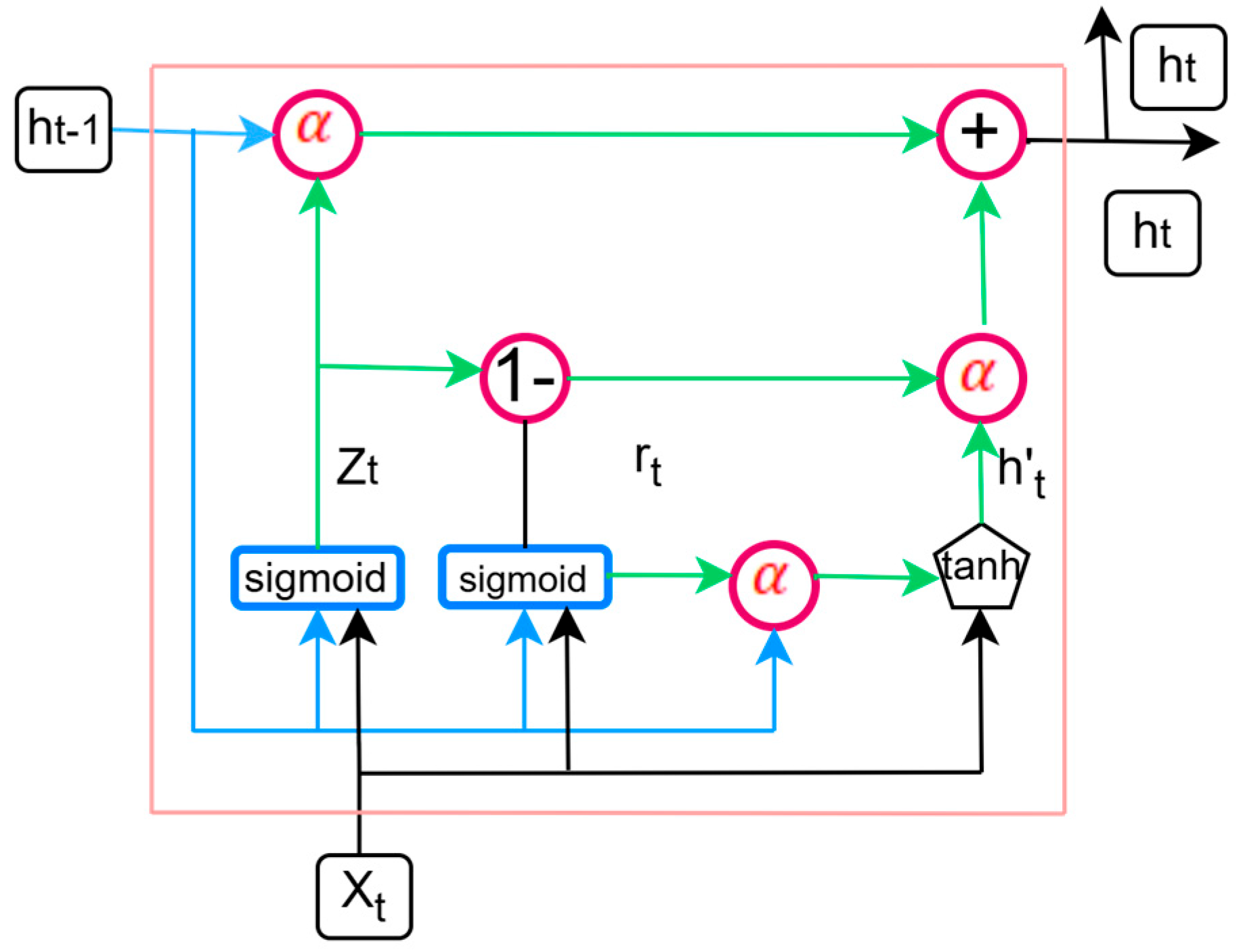
2.1.2. Gated Recurrent Unit (GRU)
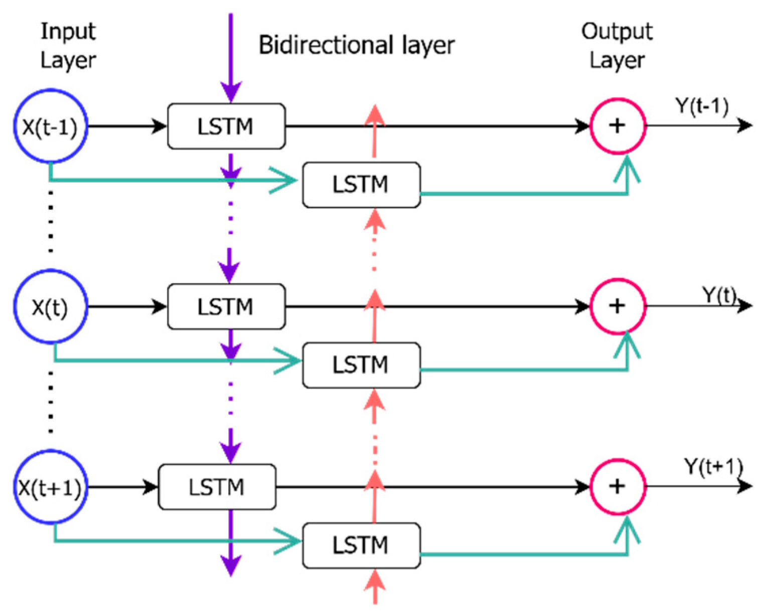
2.1.3. Bidirectional Long Short-Term Memory (BiLSTM)
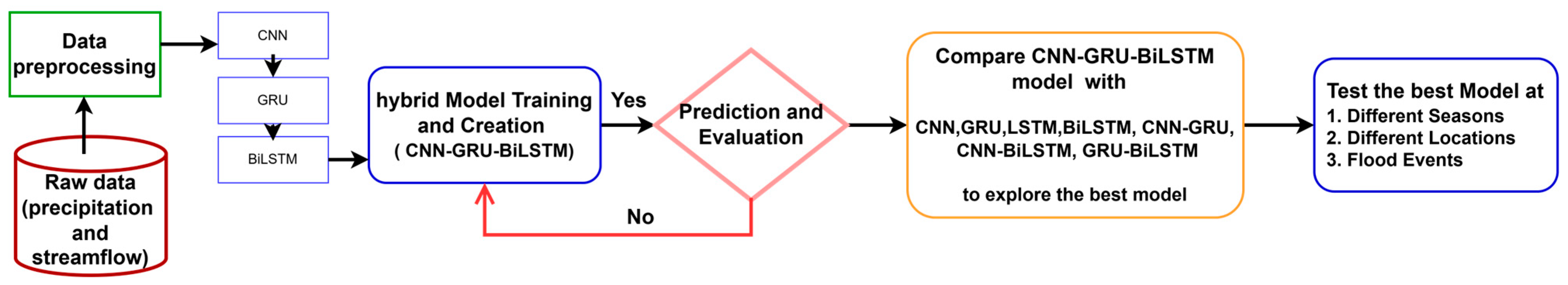
2.1.4. CNN-GRU-BiLSTM Model
2.2. Data Preparation and Model Evaluation
3. Study Area and Data
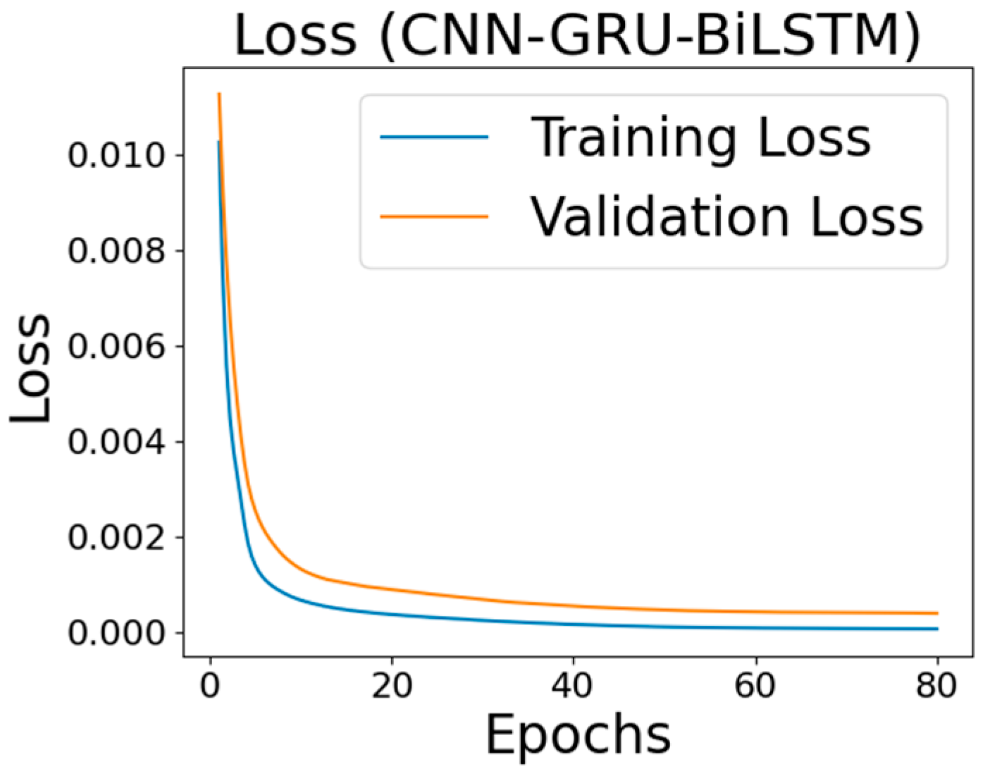
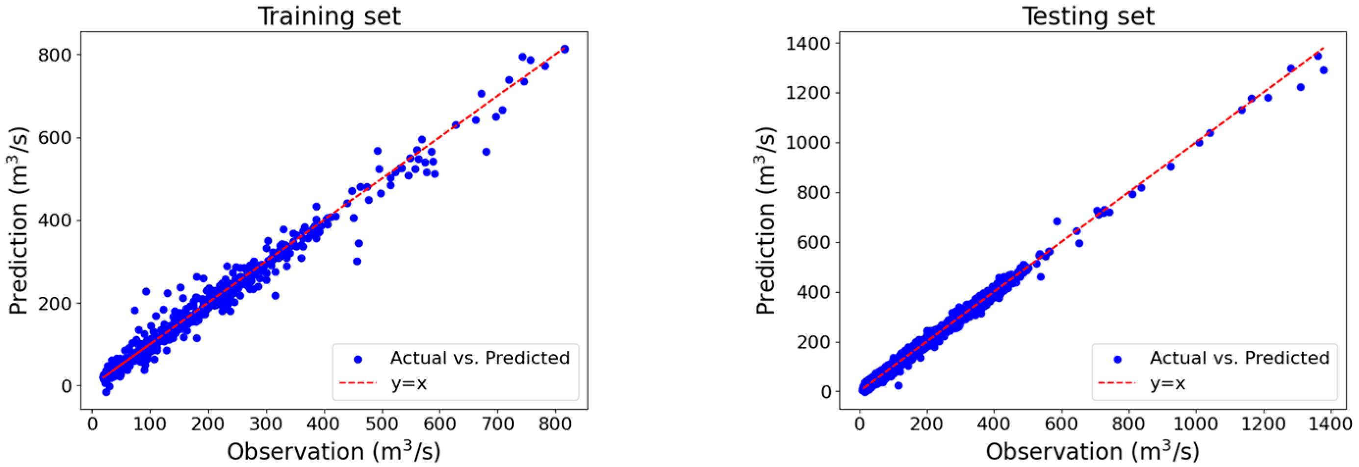
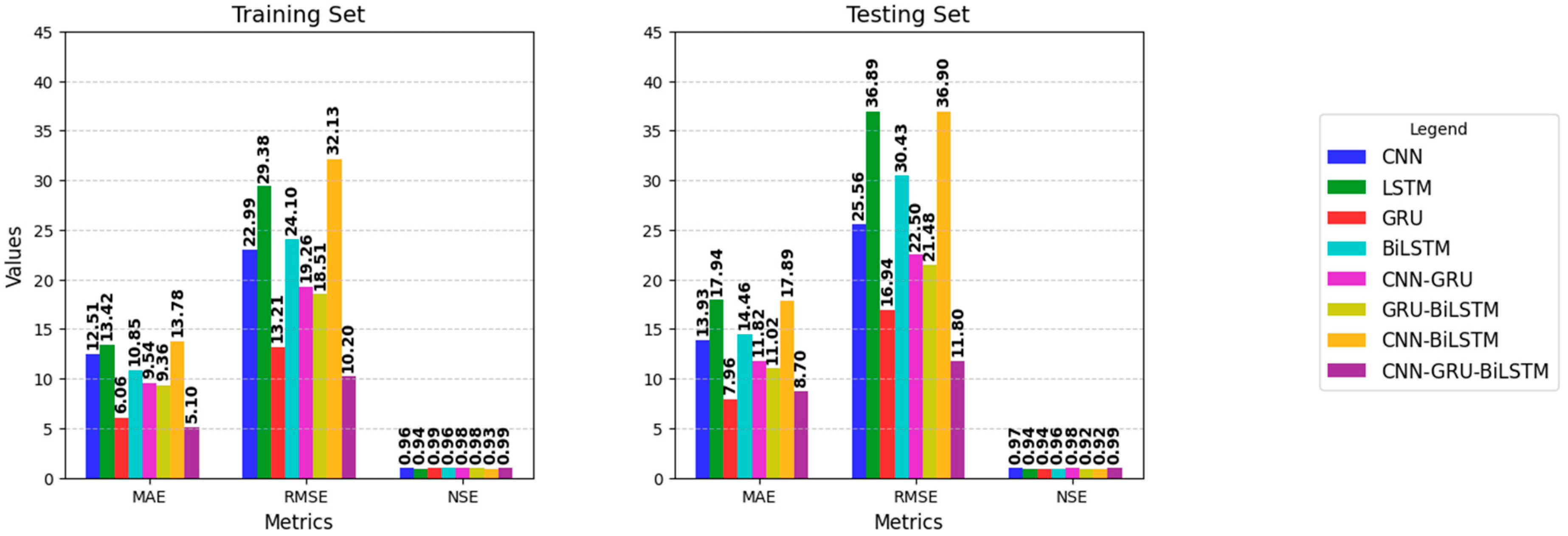
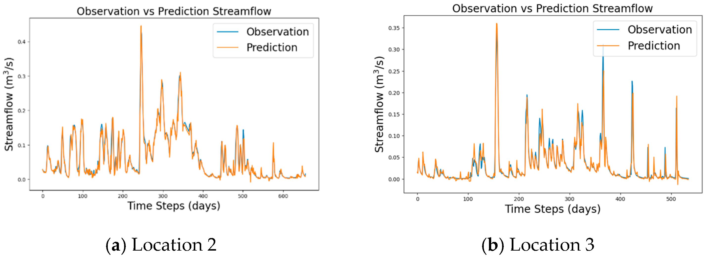
4. Results and Discussions
5. Conclusions
Author Contributions
Funding
Data Availability Statement
Acknowledgments
Conflicts of Interest
References
- Parisouj, P.; Mokari, E.; Mohebzadeh, H.; Goharnejad, H.; Jun, C.; Oh, J.; Bateni, S.M. Physics-Informed Data-Driven Model for Predicting Streamflow: A Case Study of the Voshmgir Basin, Iran. Appl. Sci. 2022, 12, 7464. [Google Scholar] [CrossRef]
- Chen, S.; Huang, J.; Huang, J.-C. Improving daily streamflow simulations for data-scarce watersheds using the coupled SWAT-LSTM approach. J. Hydrol. 2023, 622, 129734. [Google Scholar] [CrossRef]
- Beven, K. Deep learning, hydrological processes and the uniqueness of place. Hydrol. Process. 2020, 34, 3608–3613. [Google Scholar] [CrossRef]
- Yang, S.; Yang, D.; Chen, J.; Santisirisomboon, J.; Lu, W.; Zhao, B. A physical process and machine learning combined hydrological model for daily streamflow simulations of large watersheds with limited observation data. J. Hydrol. 2020, 590, 125206. [Google Scholar] [CrossRef]
- Lin, Y.; Wang, D.; Wang, G.; Qiu, J.; Long, K.; Du, Y.; Xie, H.; Wei, Z.; Shangguan, W.; Dai, Y. A hybrid deep learning algorithm and its application to streamflow prediction. J. Hydrol. 2021, 601, 126636. [Google Scholar] [CrossRef]
- Özdoğan-Sarıkoç, G.; Dadaser-Celik, F. Physically based vs. data-driven models for streamflow and reservoir volume prediction at a data-scarce semi-arid basin. Environ. Sci. Pollut. Res. 2024, 31, 39098–39119. [Google Scholar] [CrossRef]
- Li, B.; Sun, T.; Tian, F.; Ni, G. Enhancing process-based hydrological models with embedded neural networks: A hybrid approach. J. Hydrol. 2023, 625, 130107. [Google Scholar] [CrossRef]
- Latif, S.D.; Ahmed, A.N. Streamflow Prediction Utilizing Deep Learning and Machine Learning Algorithms for Sustainable Water Supply Management. Water Resour. Manag. 2023, 37, 3227–3241. [Google Scholar] [CrossRef]
- Hu, X.; Shi, L.; Lin, G.; Lin, L. Comparison of physical-based, data-driven and hybrid modeling approaches for evapotranspiration estimation. J. Hydrol. 2021, 601, 126592. [Google Scholar] [CrossRef]
- Hauswirth, S.M.; Bierkens, M.F.; Beijk, V.; Wanders, N. The potential of data driven approaches for quantifying hydrological extremes. Adv. Water Resour. 2021, 155, 104017. [Google Scholar] [CrossRef]
- Ng, K.; Huang, Y.; Koo, C.; Chong, K.; El-Shafie, A.; Ahmed, A.N. A review of hybrid deep learning applications for streamflow forecasting. J. Hydrol. 2023, 625, 130141. [Google Scholar] [CrossRef]
- Shu, X.; Ding, W.; Peng, Y.; Wang, Z.; Wu, J.; Li, M. Monthly Streamflow Forecasting Using Convolutional Neural Network. Water Resour. Manag. 2021, 35, 5089–5104. [Google Scholar] [CrossRef]
- Wang, Z.; Si, Y.; Chu, H. Daily Streamflow Prediction and Uncertainty Using a Long Short-Term Memory (LSTM) Network Coupled with Bootstrap. Water Resour. Manag. 2022, 36, 4575–4590. [Google Scholar] [CrossRef]
- Latif, S.D.; Ahmed, A.N. A review of deep learning and machine learning techniques for hydrological inflow forecasting. Environ. Dev. Sustain. 2023, 25, 12189–12216. [Google Scholar] [CrossRef]
- Zhao, X.; Wang, H.; Bai, M.; Xu, Y.; Dong, S.; Rao, H.; Ming, W. A Comprehensive Review of Methods for Hydrological Forecasting Based on Deep Learning. Water 2024, 16, 1407. [Google Scholar] [CrossRef]
- Tiwari, M.K.; Deo, R.C.; Adamowski, J.F. Short-term flood forecasting using artificial neural networks, extreme learning machines, and M5 model tree. In Advances in Streamflow Forecasting; Elsevier: Amsterdam, The Netherlands, 2021; pp. 263–279. [Google Scholar] [CrossRef]
- Ougahi, J.H.; Rowan, J.S. Enhanced streamflow forecasting using hybrid modelling integrating glacio-hydrological outputs, deep learning and wavelet transformation. Sci. Rep. 2025, 15, 2762. [Google Scholar] [CrossRef] [PubMed]
- Yu, Q.; Jiang, L.; Wang, Y.; Liu, J. Enhancing streamflow simulation using hybridized machine learning models in a semi-arid basin of the Chinese loess Plateau. J. Hydrol. 2023, 617, 129115. [Google Scholar] [CrossRef]
- He, M.; Jiang, S.; Ren, L.; Cui, H.; Du, S.; Zhu, Y.; Qin, T.; Yang, X.; Fang, X.; Xu, C.-Y. Exploring the performance and interpretability of hybrid hydrologic model coupling physical mechanisms and deep learning. J. Hydrol. 2025, 649, 132440. [Google Scholar] [CrossRef]
- Kilinc, H.C.; Yurtsever, A. Short-Term Streamflow Forecasting Using Hybrid Deep Learning Model Based on Grey Wolf Algorithm for Hydrological Time Series. Sustainability 2022, 14, 3352. [Google Scholar] [CrossRef]
- Vatanchi, S.M.; Etemadfard, H.; Maghrebi, M.F.; Shad, R. A Comparative Study on Forecasting of Long-term Daily Streamflow using ANN, ANFIS, BiLSTM and CNN-GRU-LSTM. Water Resour. Manag. 2023, 37, 4769–4785. [Google Scholar] [CrossRef]
- Fang, J.; Yang, L.; Wen, X.; Li, W.; Yu, H.; Zhou, T. A deep learning-based hybrid approach for multi-time-ahead streamflow prediction in an arid region of Northwest China. Hydrol. Res. 2024, 55, 180–204. [Google Scholar] [CrossRef]
- Pokharel, S.; Roy, T. A parsimonious setup for streamflow forecasting using CNN-LSTM. J. Hydroinform. 2024, 26, 2751–2761. [Google Scholar] [CrossRef]
- Jin, X.; Yu, X.; Wang, X.; Bai, Y.; Su, T.; Kong, J. Prediction for Time Series with CNN and LSTM. In Proceedings of the 11th International Conference on Modelling, Identification and Control (ICMIC2019), Tianjin, China, 13–15 July 2019; Lecture Notes in Electrical, Engineering. Wang, R., Chen, Z., Zhang, W., Zhu, Q., Eds.; Springer: Singapore, 2020; Volume 582, pp. 631–641. [Google Scholar] [CrossRef]
- Barzegar, R.; Aalami, M.T.; Adamowski, J. Coupling a hybrid CNN-LSTM deep learning model with a Boundary Corrected Maximal Overlap Discrete Wavelet Transform for multiscale Lake water level forecasting. J. Hydrol. 2021, 598, 126196. [Google Scholar] [CrossRef]
- Kumshe, U.M.M.; Abdulhamid, Z.M.; Mala, B.A.; Muazu, T.; Muhammad, A.U.; Sangary, O.; Ba, A.F.; Tijjani, S.; Adam, J.M.; Ali, M.A.H.; et al. Improving Short-term Daily Streamflow Forecasting Using an Autoencoder Based CNN-LSTM Model. Water Resour. Manag. 2024, 38, 5973–5989. [Google Scholar] [CrossRef]
- ArunKumar, K.; Kalaga, D.V.; Kumar, C.M.S.; Kawaji, M.; Brenza, T.M. Comparative analysis of Gated Recurrent Units (GRU), long Short-Term memory (LSTM) cells, autoregressive Integrated moving average (ARIMA), seasonal autoregressive Integrated moving average (SARIMA) for forecasting COVID-19 trends. Alex. Eng. J. 2022, 61, 7585–7603. [Google Scholar] [CrossRef]
- Le, X.-H.; Nguyen, D.-H.; Jung, S.; Yeon, M.; Lee, G. Comparison of Deep Learning Techniques for River Streamflow Forecasting. IEEE Access 2021, 9, 71805–71820. [Google Scholar] [CrossRef]
- Zhang, X.; Qi, Y.; Liu, F.; Li, H.; Sun, S. Enhancing daily streamflow simulation using the coupled SWAT-BiLSTM approach for climate change impact assessment in Hai-River Basin. Sci. Rep. 2023, 13, 15169. [Google Scholar] [CrossRef]
- Workneh, H.A.; Jha, M.K. Utilizing Deep Learning Models to Predict Streamflow. Water 2025, 17, 756. [Google Scholar] [CrossRef]
- Wei, Q.; Yang, J.; Fu, F.; Xue, L. Dynamic classification and attention mechanism-based bidirectional long short-term memory network for daily runoff prediction in Aksu River basin, Northwest China. J. Environ. Manag. 2025, 374, 124121. [Google Scholar] [CrossRef]
- Liu, Y.; Hou, D.; Bao, J.; Yong, Q. Multi-step Ahead Time Series Forecasting for Different Data Patterns Based on LSTM Recurrent Neural Network. In Proceedings of the 2017 14th Web Information Systems and Applications Conference (WISA), Liuzhou, China, 11–12 November 2017; pp. 305–310. [Google Scholar] [CrossRef]
- Sun, X.; Li, Z.; Tian, Q. Assessment of hydrological drought based on nonstationary runoff data. Hydrol. Res. 2020, 51, 894–910. [Google Scholar] [CrossRef]
- Xie, T.; Zhang, G.; Hou, J.; Xie, J.; Lv, M.; Liu, F. Hybrid forecasting model for non-stationary daily runoff series: A case study in the Han River Basin, China. J. Hydrol. 2019, 577, 123915. [Google Scholar] [CrossRef]
- Rathnayake, D.; Perera, P.B.; Eranga, H.; Ishwara, M. Generalization of LSTM CNN ensemble profiling method with time-series data normalization and regularization. In Proceedings of the 2021 21st International Conference on Advances in ICT for Emerging Regions (ICter), Colombo, Sri Lanka, 2–3 December 2021; pp. 1–6. [Google Scholar] [CrossRef]
- Nifa, K.; Boudhar, A.; Ouatiki, H.; Elyoussfi, H.; Bargam, B.; Chehbouni, A. Deep Learning Approach with LSTM for Daily Streamflow Prediction in a Semi-Arid Area: A Case Study of Oum Er-Rbia River Basin, Morocco. Water 2023, 15, 262. [Google Scholar] [CrossRef]


| Model | Architecture Type | Primary Role | Strengths in Streamflow Modeling |
|---|---|---|---|
| CNN | Feed-forward with convolutional layers | Extracts local patterns/features | Captures short-term temporal patterns and reduces noise in time series |
| GRU | Recurrent neural network with gating mechanisms | Learns sequential dependencies | Efficiently models time series with fewer parameters than LSTM, reducing overfitting risk |
| BiLSTM | Recurrent with forward and backward LSTM layers | Captures both past and future context | Improves learning of complex temporal dependencies by accessing full sequence context |
| Layer/Operation | Description |
|---|---|
| Input | (4380, 3, 1) |
| CNN layers 1 and 2 | Conv1D (64 and 32 filters, respectively, Tanh) |
| GRU layers 1 and 2 | 8 and 2 units. Tanh activation |
| BiLSTM layers 1 and 2 | 4 and 2 units, respectively. Tanh activation |
| Dense layer 1 | 30 units, Tanh |
| Output layer | Dense (1 unit regression output) |
| Compile | Adam optimizer, MSE loss function. |
| Early stopping | 4 |
| Model | Training Set | Testing Set | Training Time (s) | ||||
|---|---|---|---|---|---|---|---|
| MAE | RMSE | NSE | MAE | RMSE | NSE | 45.3 | |
| CNN | 12.51 | 22.99 | 0.965 | 13.93 | 25.56 | 0.971 | 52.1 |
| LSTM | 13.42 | 29.38 | 0.944 | 17.94 | 36.89 | 0.939 | 61.4 |
| GRU | 6.06 | 13.21 | 0.988 | 7.96 | 16.94 | 0.937 | 70.4 |
| BiLSTM | 10.85 | 24.10 | 0.962 | 14.46 | 30.43 | 0.959 | 72.3 |
| CNN-GRU | 9.54 | 19.26 | 0.976 | 11.82 | 22.50 | 0.977 | 79.8 |
| GRU-BiLSTM | 9.36 | 18.51 | 0.978 | 11.02 | 21.48 | 0.920 | 81.3 |
| CNN-BiLSTM | 13.78 | 32.13 | 0.933 | 17.89 | 36.90 | 0.920 | 93.1 |
| CNN-GRU-BiLSTM | 5.1 | 10.2 | 0.993 | 8.7 | 11.8 | 0.994 | 95.6 |
| Seasons | Training | Testing | ||||
|---|---|---|---|---|---|---|
| MAE | RMSE | NSE | MAE | RMSE | NSE | |
| Fall | 11.98 | 19.15 | 0.956 | 11.8 | 21.12 | 0.952 |
| Winter | 21.22 | 22.78 | 0.968 | 22.14 | 23.52 | 0.899 |
| Spring | 16.67 | 19.18 | 0.961 | 21.79 | 23.52 | 0.963 |
| Summer | 11.36 | 14.23 | 0.944 | 25.74 | 16.35 | 0.972 |
| Season | Training | Testing |
|---|---|---|
| Fall |  | 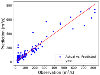 |
| Winter | 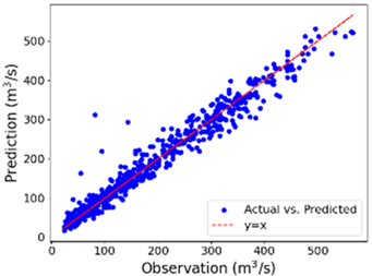 | 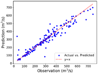 |
| Spring | 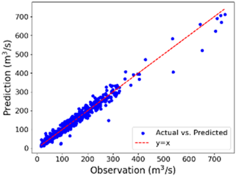 | 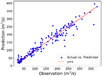 |
| Summer | 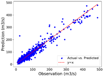 |  |
Disclaimer/Publisher’s Note: The statements, opinions and data contained in all publications are solely those of the individual author(s) and contributor(s) and not of MDPI and/or the editor(s). MDPI and/or the editor(s) disclaim responsibility for any injury to people or property resulting from any ideas, methods, instructions or products referred to in the content. |
© 2025 by the authors. Licensee MDPI, Basel, Switzerland. This article is an open access article distributed under the terms and conditions of the Creative Commons Attribution (CC BY) license (https://creativecommons.org/licenses/by/4.0/).
Share and Cite
Workneh, H.; Jha, M. Utilizing Hybrid Deep Learning Models for Streamflow Prediction. Water 2025, 17, 1913. https://doi.org/10.3390/w17131913
Workneh H, Jha M. Utilizing Hybrid Deep Learning Models for Streamflow Prediction. Water. 2025; 17(13):1913. https://doi.org/10.3390/w17131913
Chicago/Turabian StyleWorkneh, Habtamu, and Manoj Jha. 2025. "Utilizing Hybrid Deep Learning Models for Streamflow Prediction" Water 17, no. 13: 1913. https://doi.org/10.3390/w17131913
APA StyleWorkneh, H., & Jha, M. (2025). Utilizing Hybrid Deep Learning Models for Streamflow Prediction. Water, 17(13), 1913. https://doi.org/10.3390/w17131913