Groundwater Potential Mapping in Semi-Arid Areas Using Integrated Remote Sensing, GIS, and Geostatistics Techniques

Abstract

Groundwater serves as a vital resource for sustainable water supply, particularly in semi-arid regions where surface water availability is limited. This study explores groundwater potential zones in the East Desert, Qift–Qena, Egypt, using a multidisciplinary approach that integrates remote sensing (RS), geographic information systems (GIS), geostatistics, and field validation with water wells to develop a comprehensive groundwater potential mapping framework. Sentinel-2 imagery, ALOS PALSAR DEM, and SMAP datasets were utilized to derive critical thematic layers, including land use/land cover, vegetation indices, soil moisture, drainage density, slope, and elevation. The results of the groundwater potentiality map of the study area from RS reveal four distinct zones: low, moderate, high, and very high. The analysis indicates a notable spatial variability in groundwater potential, with “high” (34.1%) and “low” (33.8%) potential zones dominating the landscape, while “very high” potential areas (4.8%) are relatively scarce. The limited extent of “very high” potential zones, predominantly concentrated along the Nile River valley, underscores the river’s critical role as the primary source of groundwater recharge. Moderate potential zones include places where infiltration is possible but limited, such as gently sloping terrain or regions with slightly broken rock structures, and they account for 27.3%. These layers were combined with geostatistical analysis of data from 310 groundwater wells, which provided information on static water level (SWL) and total dissolved solids (TDS). GIS was employed to assign weights to the thematic layers based on their influence on groundwater recharge and facilitated the spatial integration and visualization of the results. Geostatistical interpolation methods ensured the reliable mapping of subsurface parameters. The assessment utilizing pre-existing well data revealed a significant concordance between the delineated potential zones and the actual availability of groundwater resources. The findings of this study could significantly improve groundwater management in semi-arid/arid zones, offering a strategic response to water scarcity challenges.

1. Introduction

Groundwater is a critical resource for sustaining life, particularly in semi-arid regions where surface water is often scarce or unavailable [1]. With increasing demand driven by population growth, urbanization, meteorological drought, and agricultural activities, effective groundwater management has become essential for ensuring long-term water security [2,3,4,5,6]. These issues associated with groundwater are of paramount importance in numerous areas characterized by elevated population densities and robust economic growth [7,8]. In arid and semi-arid environments, the scarcity of water has markedly intensified due to a deficit in surface water availability [9]. Research has indicated that groundwater resources account for over 70% of the overall water supply [10] and are progressively being depleted at a rate of approximately 545 km³ annually as a result of unsustainable extraction practices [11,12]. As asserted by [13], the majority of groundwater utilized in arid regions constitutes fossil water, which is not viable for long-term sustainability. Fossil water, a crucial non-renewable water resource, is stored within geographically isolated geological structures known as fossil aquifers. These aquifers are typically disconnected from contemporary hydrological systems and surface ecosystems [14,15]. The phenomenon of excessive pumping has resulted in a notable decline in groundwater levels [16,17]. Therefore, groundwater represents a critical element of the hydrological system, manifesting within subsurface geological formations known as aquifers [18]. As indicated by sources [19,20], the presence and accessibility of groundwater are contingent upon the recharge mechanisms, which are influenced by a multitude of factors, including lithological attributes, physiographic characteristics, drainage pattern, land utilization, and vegetative cover, in addition to climatic elements, such as precipitation, temperature, and evapotranspiration, as well as the geological context characterized by fractures and lineament features. Consequently, the potential for groundwater exhibits significant spatial and temporal variability, occasionally varying by mere meters, even within a singular aquifer. This observation substantiates the disparities in groundwater potential observed across different geographic locales [21,22].

The challenge lies in accurately identifying groundwater potential zones, which requires a detailed understanding of surface and subsurface characteristics [23,24]. The identification of groundwater potential zones is rendered complex due to a deficiency in a unified comprehension of the various environmental, climatic, and topographical factors [25,26]. Furthermore, the delineation of potential regions necessitates the evaluation of numerous geospatial variables grounded in empirical methodologies [11]. A significant number of prior studies have employed traditional methodologies for groundwater exploration, which rely on principles of geophysics, geology, and hydrogeology [27]. These conventional methods employ techniques such as geophysical (e.g., electrical resistivity, seismic) surveys, and borehole logging to identify aquifer zones and characterize groundwater systems [8,28]. While these approaches offer detailed insights into localized groundwater conditions, they are often limited in scope and practicality when applied to large or diverse terrains, such as semi-arid regions [29]. Geophysical surveys, for instance, are resource-intensive, requiring significant time, labor, and financial investment, which limits their applicability over extensive areas [30]. Geological and hydrogeological studies depend heavily on field observations, which are often constrained by challenges like inaccessible terrain, insufficient spatial coverage, and the absence of consistent data across regions. Moreover, traditional methods frequently focus on subsurface characteristics without adequately integrating surface features and environmental variables, such as land use/land cover, soil moisture, vegetation, and drainage patterns, which play critical roles in groundwater recharge processes. They also lack the ability to dynamically incorporate advancements in spatial data analysis and modeling, which are essential for addressing the complexity of groundwater systems influenced by both natural and anthropogenic factors. Another limitation lies in the absence of decision-support frameworks. Traditional approaches seldom provide mechanisms for prioritizing groundwater potential zones or systematically evaluating the interplay of multiple contributing factors. This creates challenges in holistic groundwater resource management, particularly in regions facing water scarcity and the impacts of climate variability. These gaps highlight the need for more detailed, region-specific studies that adopt integrative methodologies, combining the precision of traditional techniques with the scalability and analytical capabilities of modern geospatial technologies.

Remote sensing (RS) data have been proven to be efficient tools in locating groundwater potential zones [31,32] and in assessing its vulnerability to deterioration [33,34]. Generally, the main idea behind using remote sensing data in groundwater studies is based on calculating several surface criteria that affect groundwater behavior [31]. Among these criteria are lithology, lineament density, slope, soil moisture, and drainage density, which have formed the basis for numerous studies on groundwater potentiality in recent years [31,35,36,37]. RS and geographic information systems (GIS) have emerged as powerful tools in groundwater studies due to their ability to provide spatially extensive, high-resolution datasets [38,39,40,41,42]. However, most previous research on groundwater potential mapping in semi-arid regions has relied either on RS- and GIS-based analyses or geostatistical interpolation techniques in isolation. While these approaches offer valuable insights, they often lack a comprehensive integration of multi-source datasets, leading to limitations in accuracy and reliability. Moreover, many studies do not incorporate field validation with groundwater well data, which is essential for verifying the accuracy of predicted groundwater potential zones. To address these gaps, this study develops an integrated framework that combines RS, GIS, and geostatistics, supplemented by extensive field validation using data from 310 groundwater wells. High-resolution Sentinel-2 imagery, ALOS PALSAR DEM, and SMAP datasets were utilized alongside static water level (SWL) and total dissolved solids (TDS) measurements to enhance the accuracy of groundwater potential assessments. Additionally, GIS-based weighted overlay analysis enabled the spatial integration of multiple influencing factors, improving the precision of groundwater recharge predictions.

This research aimed to identify groundwater potential zones in the East Desert, Qift–Qena, Egypt, serving as a case study for semi-arid regions. By leveraging high-resolution satellite imagery, digital elevation models, and field data, this study established a more robust, validated, and multidisciplinary approach to groundwater potential mapping. The resulting groundwater potential map provides a valuable tool for sustainable groundwater management, supporting decision making in water resource planning and helping mitigate the impacts of water scarcity in semi-arid and arid regions.

2. Materials and Methods

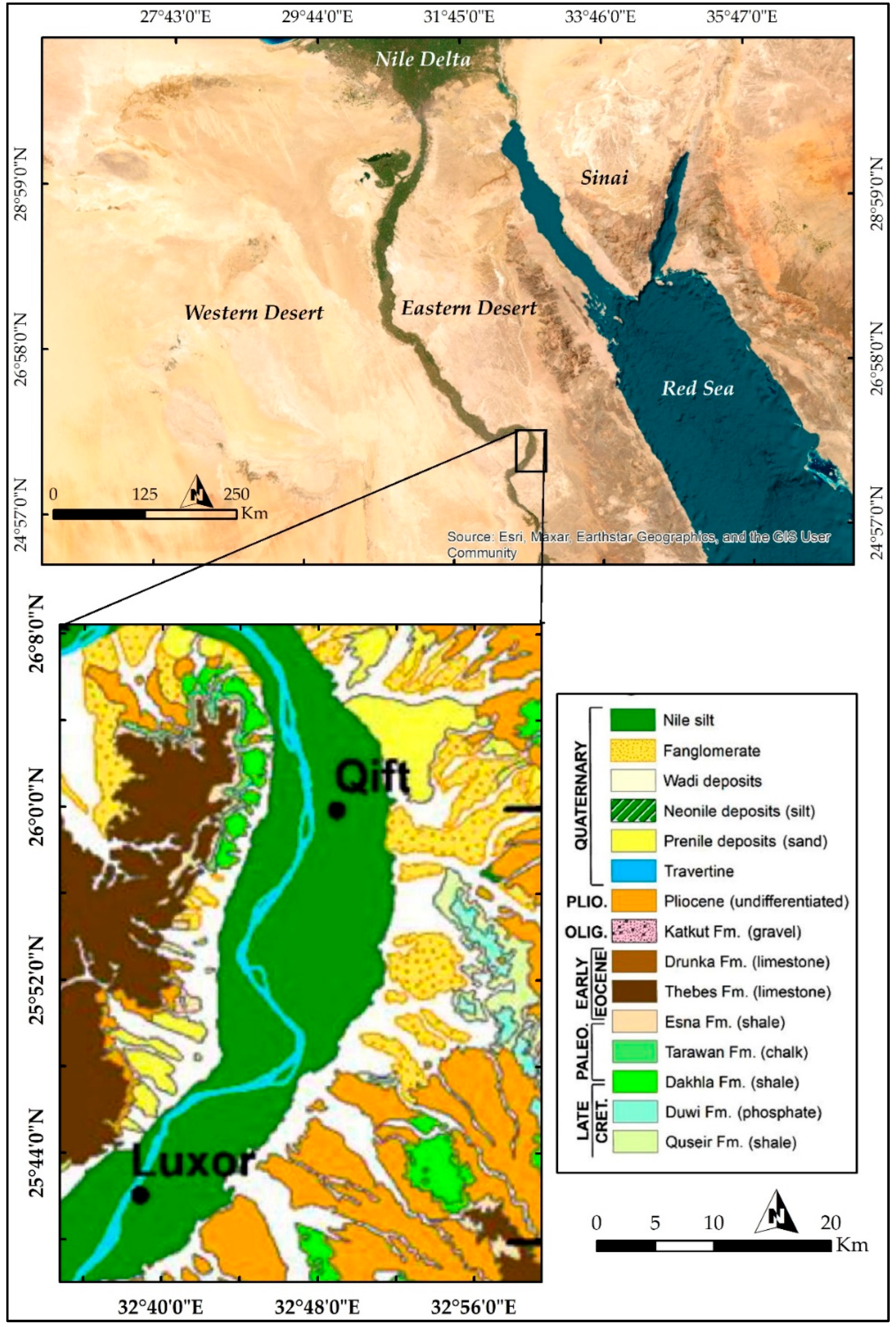
2.1. Study Area and Geological Setting

This research was carried out in the East Desert, specifically within the Qift–Qena region of Egypt. This area experiences semi-arid climatic conditions, with limited availability of surface water, making groundwater exploration essential to meet the increasing demands for domestic, agricultural, and industrial water usage. Geographically, the Qift study area lies within the Qena district, a well-developed region in southeastern Egypt, spanning approximately 2 km². It is situated between longitude 32.84° E and latitude 25.916° N, extending to longitude 32.912° E and latitude 26.058° N (Figure 1). The study area encompasses three distinct geomorphological units: the Nile floodplain and the Eastern and Western Plateaus flanking the valley [43] (Figure 1). These plateaus are primarily composed of Early Eocene massive limestone formations (brown). Along the footslopes overlooking the valley, outcrops of Cretaceous–Paleocene rocks, primarily consisting of marls and shales, are observed. The valley itself is filled with Pliocene–Quaternary alluvial and fluvial deposits. Geologically, the Qena region forms part of the Stable Shelf described by [44]. The origin of the Qena Bend is attributed by many authors to the rejuvenation of old northeast–southwest Precambrian faults that underlie northwest–southeast and north–south trends. El Kazzaz (1999) [45] proposed that this is a complex zone accommodating shifts between different segments of the Nile Valley that were caused by the reactivation of the northeast–southwest Qena–Safaga Shear Zone during the Red Sea rifting. This reactivation, involving leftward movement, diverted the Nile. While El-Gaby et al. 1988 [46] see this shear zone extending across the bend, Akawy 2002 [47] links it to the Aqaba fault system. Later studies by Akawy and Kamal El Din (2006) [48] suggested that after the Early Eocene, the area was affected by rightward movement along northwest–southeast and then north–south faults, which eventually became normal faults before the Pliocene.

2.2. Data Collection and Preparation

A comprehensive and multidisciplinary approach was adopted, integrating RS, GIS, geostatistics, and the AHP for groundwater potential locations. Multiple parameters were selected to delineate the groundwater locations. The data sources included the following:

Satellite Imagery: A cloud-free image acquired by the Sentinel-2A satellite was obtained from the European Space Agency (ESA) platform. This multispectral imagery offers a spatial resolution ranging from 10 to 60 m, depending on the specific spectral band [49,50]. Its spectral characteristics encompass a wide range, including visible, near-infrared, and shortwave infrared wavelengths, providing detailed information about the Earth’s surface. The Sentinel-2 data underwent reprojection to the WGS-84 UTM zone 36 N coordinate system, and atmospheric effects were corrected using the Sen2Cor tool to derive accurate bottom-of-atmosphere (BOA) reflectance values for subsequent analysis. Sentinel-2 imagery was utilized for land use/land cover (LULC) mapping and vegetation indices analysis. A 10- LU/LC map was generated using the latest Global Land Cover Map (GLCM) provided by Esri, which also relies on Sentinel-2 data.

Digital Elevation Model (DEM): Phased Array type L-band Synthetic Aperture Radar (PALSAR) Digital Elevation Model (DEM) acquired from the Alaska Satellite Facility (https://asf.alaska.edu/). The ALOS-PALSAR Fine Beam Single polarization (FBS, HH) RT1 product, which is radiometrically terrain-corrected with 12.5-m pixel spacing, was utilized. As an active microwave sensor operating in the L-band, PALSAR offers the advantage of day-and-night and all-weather land observation capabilities, crucial for obtaining high-resolution DEMs regardless of the environmental conditions. ALOS PALSAR DEM was utilized for deriving topographic parameters, including slope and drainage density. The L-band (1.27 GHz) synthetic aperture radar used in PALSAR is an active microwave sensor that helps to achieve high-resolution digital elevation models (DEMs).

Soil Moisture: Soil moisture was mapped using the 3 km Soil Moisture Active Passive data (SMAP/Sentinel-1 L2_SM_SP). The near-surface soil moisture (approximately the top 0–5 cm) was mapped at a 3 km spatial resolution utilizing the Soil Moisture Active Passive (SMAP) L2_SM_SP product, which synergistically combines L-band passive microwave radiometry from SMAP and active microwave radar data from Sentinel-1. While this integrated approach offers reasonable spatial detail, the fundamental sensitivity of the L-band and C-band microwave frequencies to soil moisture primarily reflects the water content within this uppermost soil layer. The effective sensing depth can be influenced by soil characteristics and vegetation cover, but the derived soil moisture estimates predominantly represent conditions in the immediate surface soil. Despite the shallow sensing depth (approximately 0–5 cm), the near-surface soil moisture data derived from the SMAP/Sentinel-1 L2_SM_SP product serve as a good surface indicator for potential groundwater resources. While not a direct subsurface measurement, surface soil moisture content can exhibit a strong correlation with underlying groundwater conditions. Therefore, mapping the surface soil moisture provides an indirect yet informative proxy for assessing the potential groundwater availability.

To strengthen soil moisture estimation, SMAP (Soil Moisture Active Passive) data were used and carefully validated prior to integration due to their relatively coarse spatial resolution. The SMAP-derived soil moisture values were compared with the soil moisture index (SMI) from Sentinel-2 imagery over the period 2020–2024. The spatial comparisons showed reasonable agreement, particularly in identifying higher moisture near the Nile Valley and lower values in the eastern desert.

While optical data provide finer spatial detail, they are limited by cloud cover and atmospheric variability. In contrast, SMAP offers stable, wide-area soil moisture estimates and has been successfully applied in similar studies [51]. Its inclusion was validated to ensure it contributed meaningfully and contextually to our methodology. By comparing both datasets, we aimed to offer the most accurate and reproducible approach possible, supporting broader applications in future groundwater assessments.

Field Data: Geostatistical analysis based on information from 310 groundwater wells, providing data on static water level (SWL) and total dissolved solids (TDS).

All datasets were pre-processed using widely approved methods to ensure data consistency and quality. This included the atmospheric correction of Sentinel-2 imagery using the Sen2Cor processor, projection harmonization to WGS-84 UTM Zone 36N, resampling and filling of the DEM data, and quality checks on the well data. All datasets were converted into raster format and integrated within a GIS environment (ArcMap v.10.8) for subsequent groundwater potential mapping.

2.3. Thematic Layer Generation

Expert consultation involved engaging both domain specialists and local residents familiar with the hydrogeological conditions of the study area. Experts, including geologists, hydrologists, and water resource professionals, were asked to evaluate and rank the importance of various factors influencing groundwater potential in the study area. Their insights were complemented by local knowledge, particularly regarding land use practices, water availability, and recharge behavior. Based on this consultation, the most important factors identified for groundwater potential in this study area were land use/land cover, vegetation indices, soil moisture, drainage density, slope, and elevation. The experts rated each criterion relative to the others, and these ratings informed the weighting and prioritization of the thematic layers used in the analysis.

Although rock type is a widely recognized factor in groundwater potential mapping, it was not included in the current study due to the unique characteristics of the study area. Significant heterogeneities and localized variations in the surface geology, often driven by anthropogenic influences, complicate the use of generalized lithological data. Additionally, lithofacies variations within single units and undifferentiated lithologies, such as the extensive Pliocene formations depicted in the geological map, limit the reliability of rock type as a discriminating layer. Moreover, proximity to the Nile Valley and intensive irrigation activities can facilitate recharge across various lithologies, reducing the spatial consistency needed to treat rock type as a meaningful predictor.

Given the nature and specific characteristics of the study area, a set of thematic maps was developed to represent the key factors influencing groundwater recharge potential. These thematic layers were generated, analyzed, and prioritized based on expert consultation and the geologic and geomorphologic attributes of the terrain.

Land Use/Land Cover (LULC): The LULC was classified from Sentinel-2 imagery using supervised classification techniques. The LULC significantly influences groundwater recharge by affecting infiltration rates and runoff. For example, urban areas with impervious surfaces, like concrete and asphalt, promote rapid runoff, reducing the amount of water that can infiltrate and recharge groundwater. Agricultural practices also play a role, with certain methods increasing or decreasing recharge depending on soil management and irrigation. Thus, it was given special importance in the current research as the study area has a significant number of urbanized areas.

Vegetation Indices: The normalized difference vegetation index (NDVI) was computed to assess vegetation cover. The NDVI was calculated using a Sentinel-2 scene acquired in 2023 to assess the vegetation cover in the study area, which indirectly supports groundwater potential analysis. The NDVI was derived by applying the standard equation NDVI = (NIR − RED)/(NIR + RED), where NIR refers to the near-infrared band and RED refers to the red band. For Sentinel-2 imagery, Band 8 (842 nm) was used as the NIR band, and Band 4 (665 nm) as the RED band. This index helps in identifying areas with higher vegetation density, which may indicate better conditions for groundwater recharge due to enhanced infiltration and reduced runoff. Vegetation cover, as indicated by the NDVI, is a strong indicator of evapotranspiration and infiltration. Areas with dense vegetation tend to have higher evapotranspiration rates, which can reduce the amount of water available for groundwater recharge. However, vegetation also enhances soil permeability and reduces surface runoff, which can increase infiltration. Higher NDVI values often indicate areas where water is available to support plant life, suggesting potential groundwater presence. In this research, vegetation was also easily visualized through simple false color combination (FCC), which clearly distinguishes vegetation from other exposed covers.

Soil Moisture: SMAP data were processed to visualize and quantify spatial variations in the soil moisture. Soil moisture is a direct indicator of water availability. Higher soil moisture levels generally indicate a greater potential for water to infiltrate and reach the water table. Its spatial distribution provides valuable insights into areas with higher recharge potential.

Drainage Density: The drainage network was derived from ALOS PALSAR DEM and using standard hydrological modeling tools available in the ArcGIS Spatial Analyst toolbox, specifically under the Hydrology toolset. The workflow included a sequence of models commonly used for DEM-based hydrological analysis, including Fill (to remove sinks), Flow Direction, Flow Accumulation, and Stream Definition. These tools were applied to the ALOS PALSAR DEM to extract the drainage network and calculate the drainage density across the study area. Drainage density reflects the efficiency of water removal from a watershed. Areas with high drainage density, characterized by numerous closely spaced streams, tend to have rapid runoff and limited infiltration, reducing groundwater recharge. Conversely, areas with low drainage density, with fewer and more widely spaced streams, allow more time for water to infiltrate, increasing recharge potential. Drainage density also indicates the permeability of the underlying geology, influencing how quickly water can move through the subsurface.

Slope and Elevation: Extracted from DEM data to understand topographic influences on groundwater recharge. Slope and elevation are fundamental topographic factors that influence groundwater recharge by controlling runoff and infiltration. Steeper slopes promote rapid runoff, reducing the time for water to infiltrate and recharge groundwater. Conversely, gentler slopes allow more time for infiltration. Elevation dictates the overall flow of water, with higher elevations acting as recharge areas and lower elevations as discharge areas. Elevation also helps define the drainage pattern of the area.

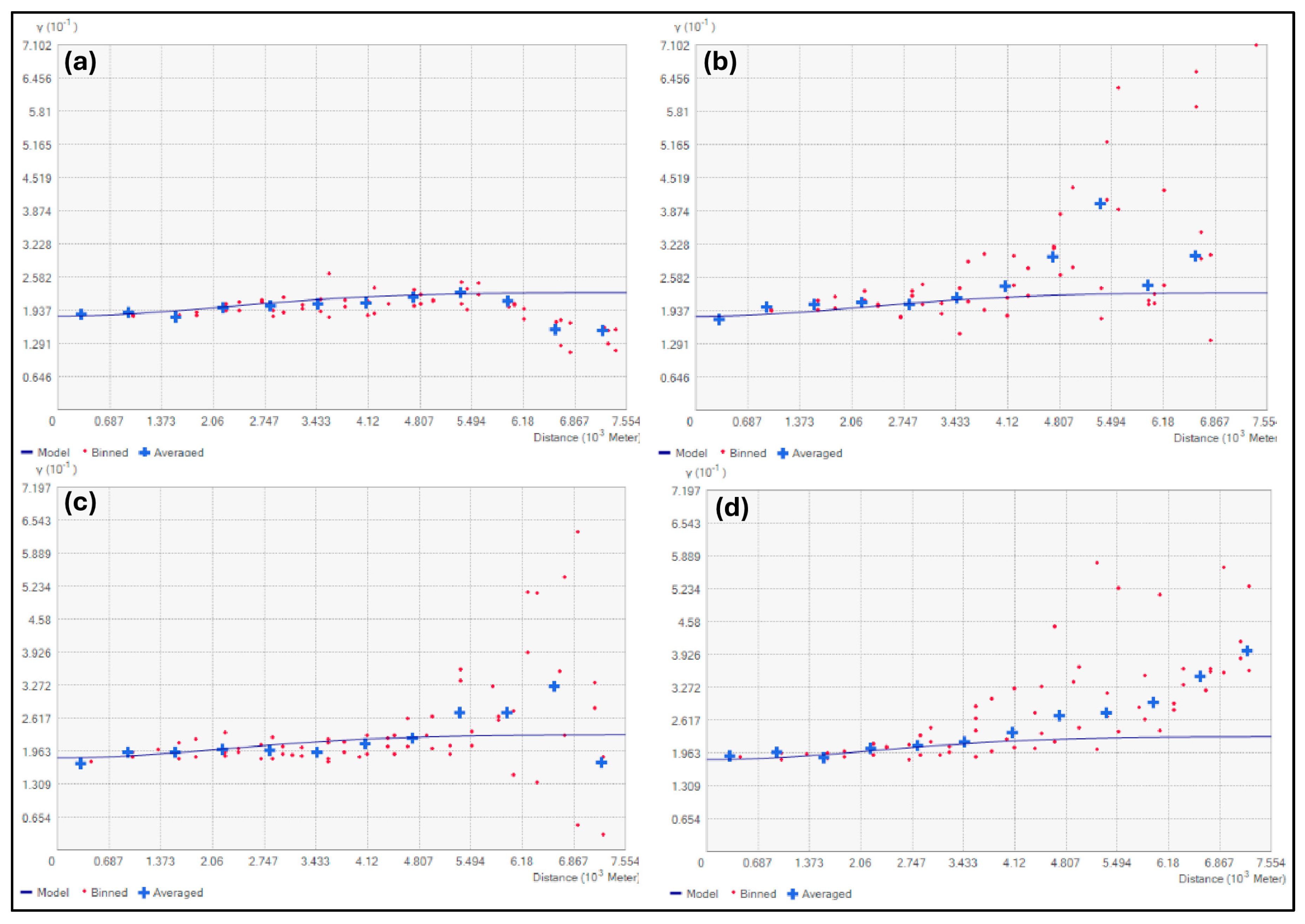
2.4. Geostatistical Analysis Theory

The geostatistical analysis in this study began with exploratory data analysis (EDA) to assess the spatial characteristics and distribution patterns of SWL and TDS. The cumulative frequency distributions of these parameters were evaluated, and transformations, such as log normalization, were applied to better approximate normal distributions, facilitating more accurate geostatistical modeling [52]. The analysis involved the derivation and modeling of empirical variograms for the transformed parameters. Empirical variograms describe the spatial continuity of the data by quantifying the variance among values at varying distances [53,54]. The standard equation used to calculate the empirical variogram is as follows:

$$\gamma \left(h\right)={\displaystyle \frac{1}{2N\left(h\right)}}\sum _{i=1}^{N\left(h\right)}{\left[\left(z\left(x_i\right)-z\left(x_i+h\right)\right)\right]}^2$$

(1)

where $\gamma \left(h\right)$ is the semivariance for lag distance $h$, $N\left(h\right)$ is the number of pairs of sample points separated by $h$, and $z\left(x_i\right)$ and $z\left(x_i+h\right)$ are the values at two points separated by $h$.

Model variograms, such as spherical and exponential models, were fitted to the empirical variograms:

$$\gamma \left(h\right)=n+s\left(1-exp\left(-{\displaystyle \frac{h}{r}}\right)\right)$$

(2)

where $n$ is the nugget effect, $s$ is the sill, and $r$ represents the practical range. The model parameters were estimated using maximum likelihood estimation techniques. Cross-validation was employed to assess the model’s accuracy, wherein data points were sequentially removed and predicted using kriging interpolation. The standardized differences between the observed and predicted values were expected to be unbiased and follow a standard normal distribution.

For prediction, ordinary kriging (OK) was employed as a least-squares linear regression estimator. This method assigns weights ${\lambda }_i$ to each data point in a given neighborhood, ensuring unbiased estimates and minimal error variance:

$$Z^{\ast }\left(x\right)=\sum _{i=1}^N{\lambda }_{i}z\left(x_i\right)$$

(3)

where $N$ is the number of neighboring points considered, and ${\lambda }_i$ are the kriging weights determined by minimizing the estimation variance.

Interpolation maps of SWL and TDS were generated using QGIS, applying the kriging technique with six neighboring points and a smoothing factor of 0.2. The error variance ${\sigma }_E^2$ was calculated as follows:

$${\sigma }_E^2=Var\left[Z^{\ast }\left(x\right)\right]+\mu$$

(4)

where $\mu$ is a Lagrange multiplier. These predictive maps provide insights into the spatial distribution of groundwater quality parameters, supporting informed decision making in groundwater potential assessment. This comprehensive geostatistical workflow facilitated a robust understanding of the spatial patterns and trends in the groundwater parameters, laying the foundation for future environmental and hydrological research.

2.5. Analytical Hierarchy Process (AHP) and Groundwater Potential Mapping

Expert input was obtained through consultations with both subject-matter specialists and local inhabitants who possess practical knowledge of the region’s hydrogeological setting. Professionals such as geologists, hydrologists, and water resource experts participated in evaluating and ranking the relative significance of factors influencing groundwater potential. This collaborative consultation process led to the identification of land use/land cover (lowest rank), vegetation indices, soil moisture, drainage density, slope, and elevation (highest rank) as the most influential factors in the study area. Each factor was rated in comparison to the others, and these ratings were used to guide the weighting and hierarchical structuring of the thematic layers in the AHP-based analysis. The analytical hierarchy process (AHP) technique was employed to assign weights to the selected thematic layers (LU/LC, NDVI, soil moisture, drainage density, slope, and elevation) based on their relative influence on groundwater potential. The AHP is a well-established and efficient multi-criteria decision-making (MCDM) approach that has been widely recommended in similar groundwater potential mapping (GWPM) studies [55,56]. Previous research has shown that multiple parameters, such as NDVI, soil moisture, slope, and LU/LC, significantly contribute to delineating groundwater potential zones [57].

Geographic information systems (GIS) technology was utilized as the core platform for integrating the weighted thematic layers and producing the final groundwater potential map. Following the determination of criterion weights through the AHP process, the weighted linear combination (WLC) [58,59] method was employed to overlay thematic maps based on their assigned importance. This process involved three key steps: (1) the reclassification of all thematic layers onto a standardized scale to ensure consistency; (2) application of the WLC method, which aggregated the reclassified layers using their respective AHP-derived weights; and (3) the delineation of groundwater potential zones by classifying the resulting composite map into categories ranging from low to high groundwater potential. This integrative GIS-based approach enabled the spatial representation of groundwater potential across the study area with enhanced precision.

2.6. Validation and Accuracy Assessment

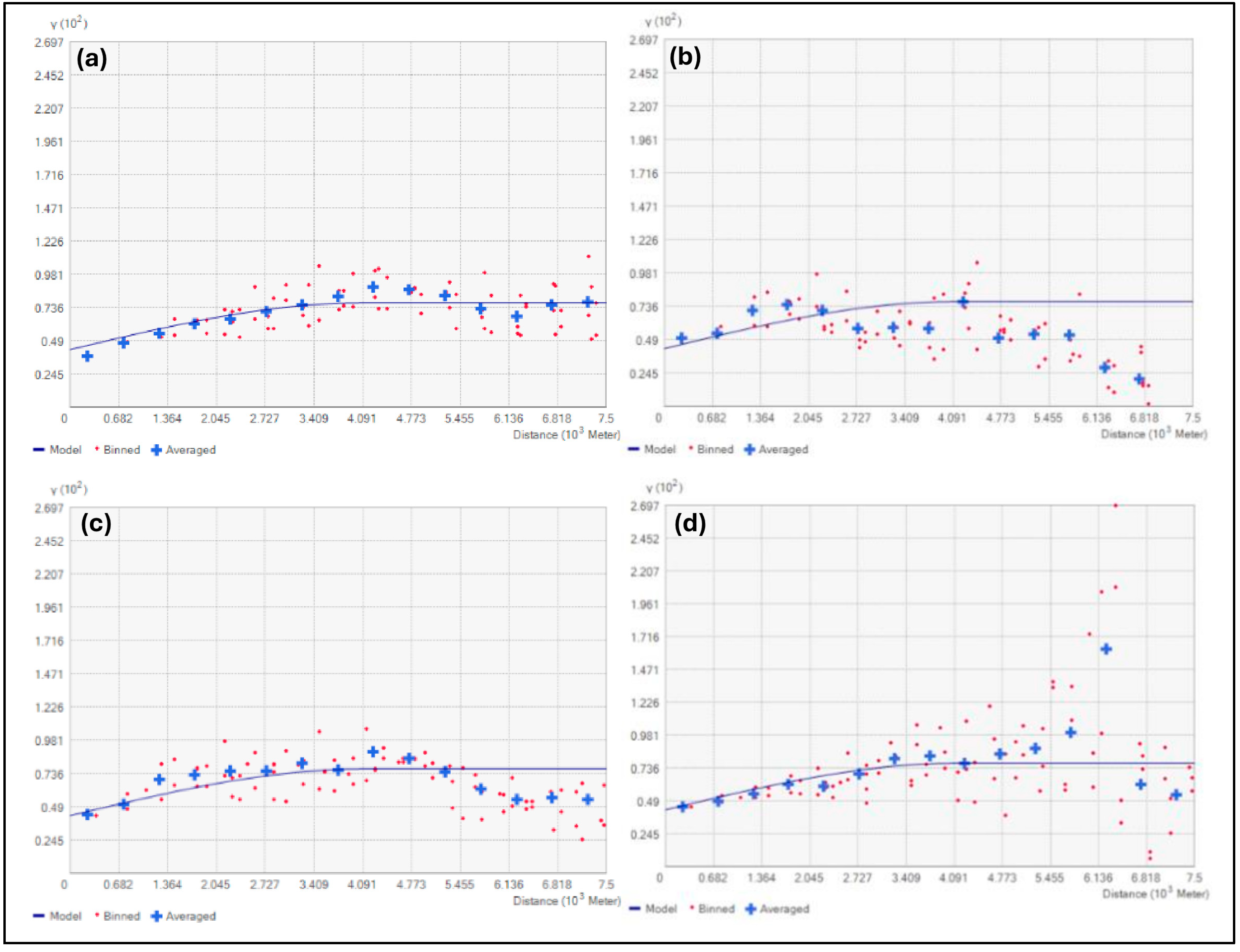
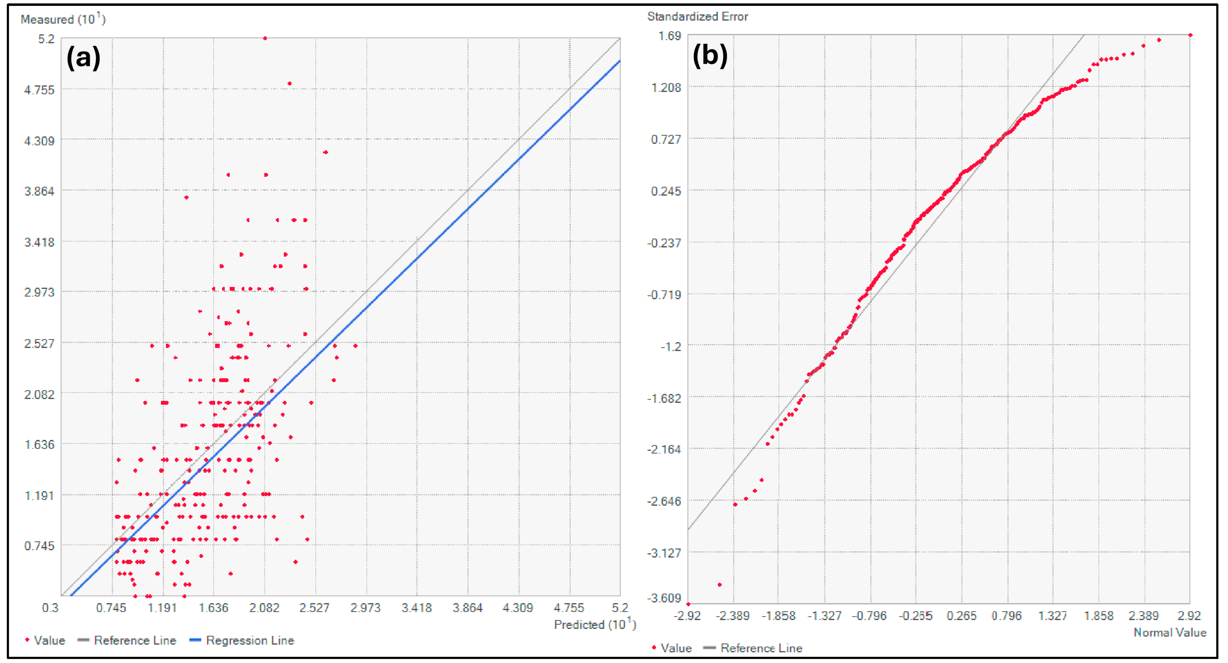
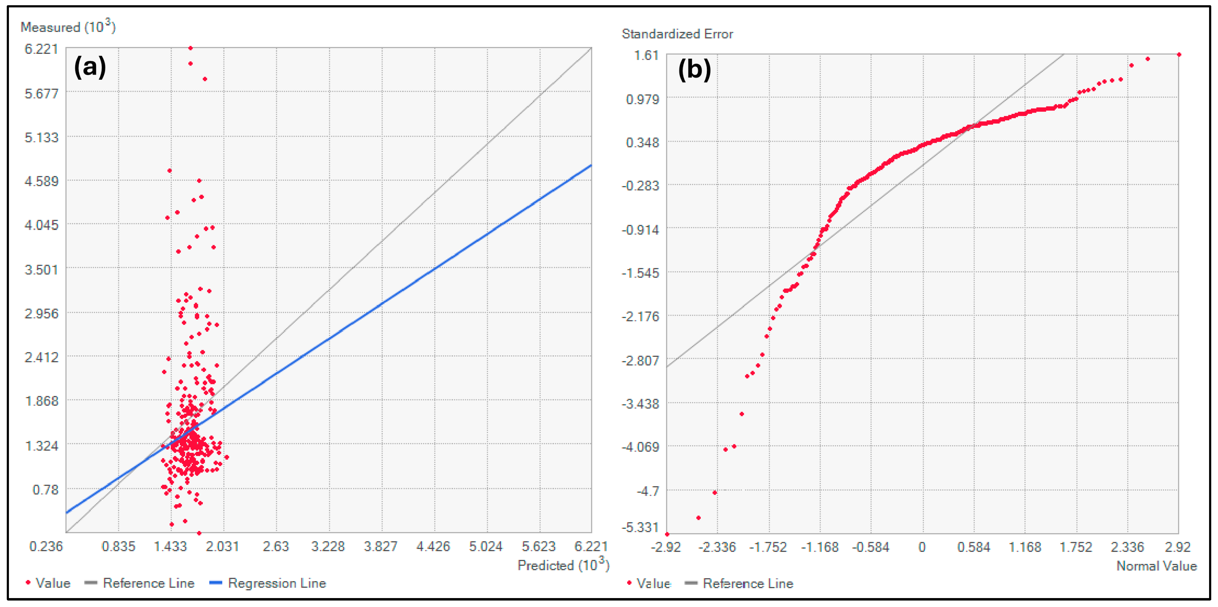
2.6.1. Geostatistical Model Validation

The validation of the groundwater potential model was supported by a comprehensive field-based dataset obtained from the Ministry of Water Resources and Irrigation (MWRI), Egypt, which was used to construct and evaluate the geostatistical model. This dataset includes observations from 310 groundwater wells distributed across the study area, providing measured values for both static water level (SWL) in meters and total dissolved solids (TDS) in parts per million (ppm). The broad spatial coverage of these wells ensures that various geomorphological and hydrogeological settings are well represented, contributing to the reliability of the model validation process.

Table 1. Statistical summary of the verification dataset.

Parameter	Statistical Index
	Count	Mean	Std	Min	Max	Skewness	Kurtosis	IQR	Range
SWL	310	15.867	8.9	3	52	1.0080	0.8331	11	49
TDS	310	1661.5	909.7	236	6221	2.1856	2.1856	664	5985

presents a detailed statistical summary of the verification dataset, including descriptive indices that reflect central tendency, dispersion, and distribution shape. These statistics provide insight into the spatial variability and potential uncertainty of the observed groundwater parameters.

For SWL, the measured values ranged from 3 m to 52 m, with a mean of 15.87 m and a standard deviation of 8.9 m, indicating moderate variability in groundwater depth across the region. The distribution is positively skewed (skewness = 1.008), suggesting the presence of a number of deeper wells, particularly in higher-elevation or recharge-limited zones. The kurtosis value of 0.83 indicates a slightly flatter-than-normal distribution. The interquartile range (IQR) was 11 m, and the total range was 49 m, highlighting considerable variation in aquifer conditions.

For TDS, the values ranged from 236 ppm to 6221 ppm, with a mean of 1661.5 ppm and a standard deviation of 909.7 ppm, reflecting substantial heterogeneity in groundwater salinity. The distribution is strongly right-skewed (skewness = 2.19) and leptokurtic (kurtosis = 2.19), indicating the presence of significant outliers with elevated salinity levels, possibly due to localized geological or anthropogenic influences. The IQR was 664 ppm, and the range spanned 5985 ppm, emphasizing the importance of incorporating water quality variability into groundwater potential assessments.

In addition to the statistical summaries, the following metrics were employed to evaluate model accuracy:

• Accuracy Metrics: Both the root mean square error (RMSE) and mean absolute error (MAE) were calculated to quantify prediction performance.

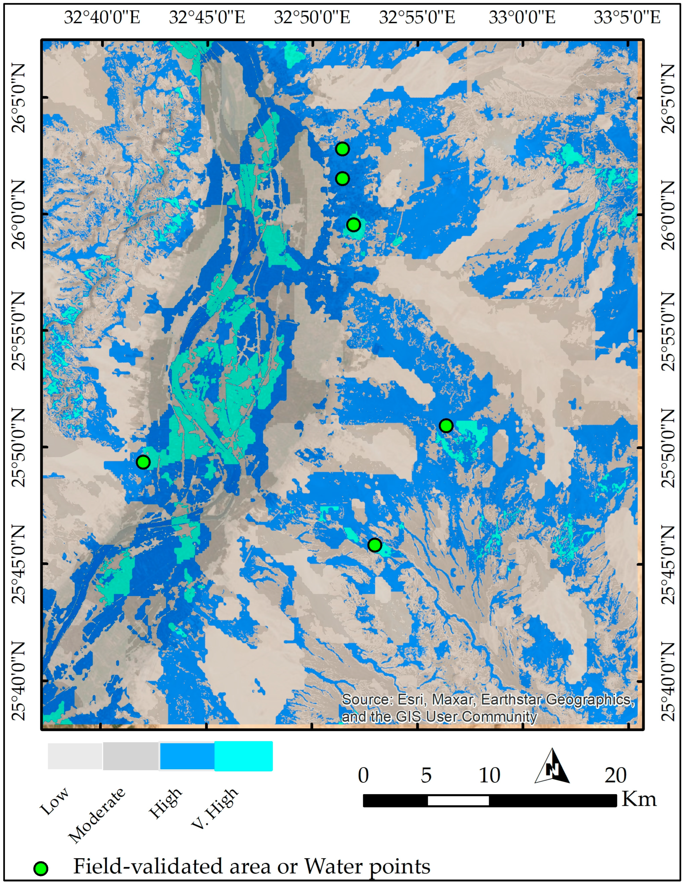
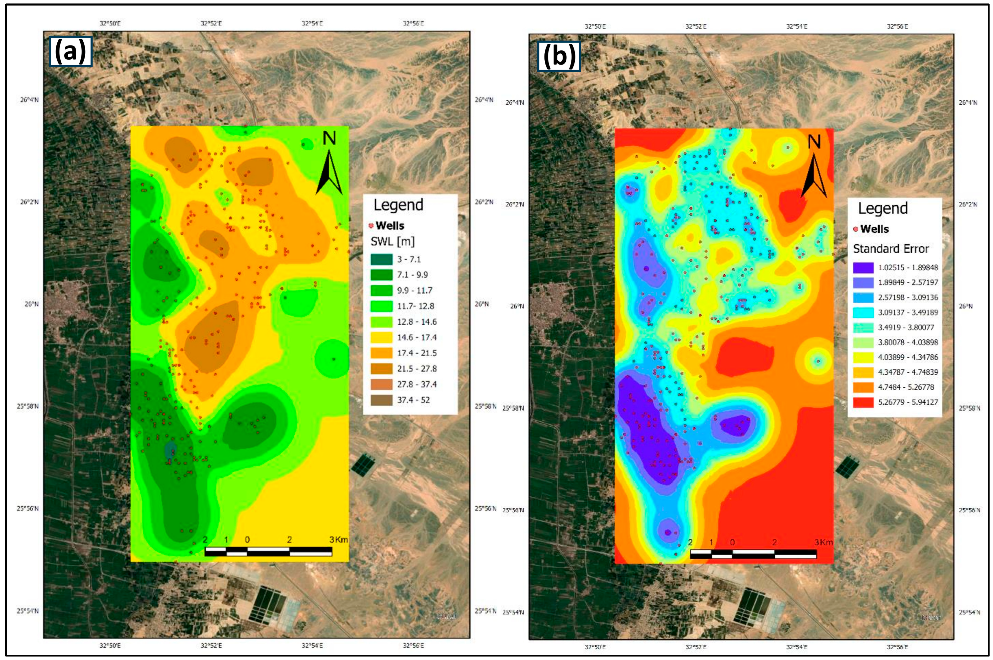
2.6.2. Field Validation

Ground-truthing was conducted by comparing the predicted zones with on-site measurements. Six verification points were spatially distributed across the study area, specifically located within zones identified as having high to very high groundwater potential based on the GWPM results. These points were selected to represent a range of hydrogeological settings and were either verified through direct field visits or confirmed to host existing water wells. The verification process involved cross-referencing the mapped zones with actual groundwater presence and well performance, thereby validating the model’s predictive capability.

3. Results and Discussion

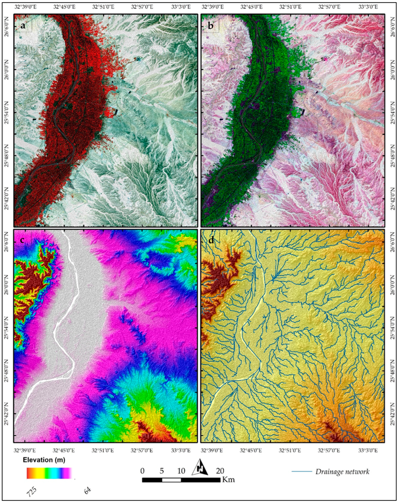
3.1. Remote Sensing

The current research integrated several remote sensing datasets, including Sentinel-2 data, ALOS PALSAR data, and the 3-km Soil Moisture Active Passive data (SMAP/Sentinel-1 L2_SM_SP). Launched by ESA, a pair of analogous satellites positioned within the same orbit forms the cornerstone of the Copernicus Sentinel-2 program. Sentinel-2 satellites provide high-resolution imagery up to 10 m with 13 spectral bands through their multispectral imager. For the purpose of the current research, the S2A_MSIL2A scene was utilized to better understand the characteristics of the study area. Many image processing methods were used to distinguish between the exposed land covers in the research area, but false color composites (FCCs) were chosen because they are the most straightforward and produce easily understood images. For example, a Sentinel-2 FCC of 8-4-3 in RGB used these wavelengths, including NIR, to clearly show the red vegetation cover. Furthermore, all of the exposed lithologies can be reasonably identified using Sentinel-2’s RGB FCC of 12/6/2. Through these FCCs (Figure 2a,b), the vegetation, water, and lithologies were clearly distinguished. The elevations (Figure 2c) were visualized using the ALOS-PALSAR DEM RT1 (Radiometric Terrain-Corrected) with pixel spacing of 12.5 m. The drainage pattern within the study area is entirely dictated by elevation, as illustrated in Figure 2d. This topographic control manifests in the direction and density of water flow, with higher elevations acting as water divides, and lower elevations (Nile valley) serving as accumulation zones. Consequently, the arrangement of streams and rivers directly reflects the underlying elevation gradients, highlighting the fundamental influence of topography on the hydrological network and in the ground water potentiality within the study area.

Further analysis of the drainage density (Figure 3a) and slope (Figure 3b) reinforces this relationship. Higher drainage densities typically correlate with steeper slopes, indicating rapid runoff and limited infiltration. Conversely, areas with lower drainage densities and gentler slopes exhibit slower runoff and increased potential for water accumulation. This interplay between drainage density and slope directly impacts the soil moisture content (Figure 3c), where areas of higher moisture often coincide with lower slopes and denser drainage networks. Finally, the distribution of the LULC (Figure 3d) reveals how human activities and natural vegetation patterns interact with these hydrological characteristics, influencing runoff, infiltration, and ultimately, groundwater recharge.

By integrating these findings (elevation, drainage patterns, drainage density, slope, soil moisture, and LULC), a comprehensive groundwater potentiality map was developed. This integration was achieved through the AHP. The resulting groundwater potentiality map, presented in Figure 4, spatially delineates areas of varying groundwater potential, ranging from high to low, reflecting the combined influence of these factors.

The groundwater potential map (Figure 4) and the calculated area percentages (from GIS) reveal several key insights into the distribution and influencing factors of groundwater resources within the study area. The analysis indicates a notable spatial variability in groundwater potential, with “high” (34.1%) and “low” (33.8%) potential zones dominating the landscape, while “very high” potential areas (4.8%) are relatively scarce. The limited extent of “very high” potential zones, predominantly concentrated along the Nile River valley, underscores the river’s critical role as the primary source of groundwater recharge. This finding aligns with the understanding of arid and semi-arid environments, where perennial rivers, like the Nile, serve as major conduits for aquifer replenishment through infiltration [60]. The consistent supply of water from the river, coupled with irrigation practices in the adjacent areas, contributes to the localized zones of high groundwater accumulation. The network of irrigation channels, while essential for agriculture, also inadvertently facilitates groundwater recharge through seepage, further explaining the high potential observed in these areas. The influence of topography on groundwater potential is evident in the spatial distribution patterns. Lower-lying areas, particularly the Nile valley and its floodplains, naturally act as zones of water accumulation, receiving both direct river recharge and runoff from surrounding higher elevations.

As noted in the data sources, the drainage patterns within the study area are “entirely dictated by elevation,” with higher elevations acting as water divides and lower elevations serving as accumulation zones. This topographical control manifests in the higher groundwater potential observed in these low-lying regions. Conversely, areas with steeper slopes and higher elevations, characterized by higher drainage densities, exhibit lower infiltration rates and increased runoff, resulting in the “low” groundwater potential observed across a substantial portion of the study area. The distribution of the LULC also plays a significant role in shaping groundwater potential. Agricultural areas, particularly those under irrigation, are often associated with higher recharge rates due to the application of irrigation water. However, other land use types, such as urban areas or barren lands, may exhibit lower infiltration rates and reduced groundwater recharge.

The application of the AHP in this study provided a systematic framework for integrating the various influencing factors and generating the groundwater potentiality map. The AHP’s ability to incorporate both quantitative data (e.g., elevation, slope) and qualitative factors (e.g., LULC) allowed for a comprehensive assessment of the groundwater potential. However, it is important to acknowledge that the accuracy of the map and the calculated percentages is dependent on the quality and resolution of the input data, as well as the assigned weights in the AHP analysis. The findings of this study have significant implications for water resource management in the region. The identification of “high” and “very high” potential zones provides valuable information for prioritizing areas suitable for groundwater extraction and development. Conversely, the delineation of “low” potential areas highlights the need for careful water resource planning and the exploration of alternative water sources. Sustainable groundwater management strategies should consider the spatial variability in groundwater potential, the influence of the Nile River, and the impact of human activities on recharge rates.

3.2. Geostatistical Analysis Results

The histograms for SWL and TDS distributions and their log-transformed are shown in Figure 5. Figure 5a,c show the original distributions of the SWL and TDS, respectively. Both exhibit a positive skew, indicating a concentration of values toward the lower end of the range and a long tail extending toward higher values. This suggests that the data are not normally distributed and have high variability. The distributions following log transformation are shown in Figure 5b,d. The transformed SWL and TDS data exhibit a more symmetrical, bell-shaped curve, approximating a normal distribution. The variability is also reduced after the transformation. This suggests that the log transformation effectively normalized the data, making it more suitable for geostatistical analyses that assume normality.

Figure 6 and Figure 7 display the directional empirical variograms for the log-transformed SWL and TDS data, respectively, calculated using a 500 m lag. Omnidirectional variograms for both variables are presented in Figure 8, with a focus on the short-range variation (also using a 500 m lag) to illustrate convergence toward the nugget effect. Visual inspection of the spatial correlation patterns in the SWL and TDS datasets, as shown in the respective figures, indicates the absence of significant anisotropy. Therefore, an isotropic spherical variogram model was selected as the most appropriate representation of spatial dependence. This model was fitted to the data using the restricted maximum likelihood (REML) estimation method, which provides robust parameter estimates by minimizing bias in small sample sizes. The estimated model parameters, including nugget, sill, and range, are summarized in

Table 2. Parameters of the fitted isotropic spherical variogram models for SWL and TDS, estimated using the restricted maximum likelihood.

Parameters	SWL	TDS
Lag size	500	500
Number of lags	12	12
Nugget	33	1.8
Sill	74	2.3
Range	4330	5475

. As expected, the nugget and range parameters, which characterize short-range variability, are primarily determined by the behavior of the empirical variogram near the origin. To assess the suitability of the selected variogram model, a comparison was conducted among three commonly used theoretical models: spherical, exponential, and Gaussian. Each model was fitted to the empirical variograms of both the SWL and TDS datasets, and their performance was evaluated using cross-validation metrics, including the root mean square error (RMSE), mean absolute error (MAE), and mean standardized error. The spherical model consistently yielded the lowest RMSE and MAE, along with standardized error values closest to zero, indicating both accuracy and lack of systematic bias. In contrast, the Gaussian and exponential models showed slightly higher error values and less favorable standardized residuals. These statistically meaningful differences affirm that the spherical model provides the most reliable spatial predictions for both variables in this study. Therefore, the selection of the spherical model was not only guided by visual inspection of isotropy but also validated by quantitative performance criteria.

For the cross-validation of SWL and TDS interpolation variables, the accuracy of the kriging interpolation models for both SWL and TDS was evaluated using leave-one-out cross-validation in ArcGIS Pro [53,54], a robust method that assesses model performance by systematically removing each data point and predicting its value using the remaining dataset. The cross-validation statistics for both variables demonstrate the reliability and suitability of the applied geostatistical approach.

For SWL (

Table 3. Cross-validation performance metrics for the SWL prediction surface, including error statistics that evaluate the accuracy, bias, and reliability of the kriging interpolation model.

Index	Value
Count	286
Mean Absolute Error (MAE)	0.040
Root Mean Square Error (RMSE)	3.135
Mean Standardized	0.015
Root Mean Square Standardized (RMSS)	0.935

), the model was validated using 286 data points. The mean absolute error (MAE) was exceptionally low at 0.040, indicating a high degree of agreement between the predicted and observed values. The RMSE was calculated as 3.135, reflecting minimal dispersion of prediction errors and suggesting that the model performs well even for larger deviations. Furthermore, the mean standardized error was 0.015, very close to zero, confirming the absence of significant systematic bias in the predictions. The root mean square standardized (RMSS) value of 0.935, being close to the ideal value of 1, indicates that the kriging standard errors are well calibrated and that the uncertainty estimates are statistically reliable. The associated prediction and normal Q-Q plots (Figure 9) visually support the consistency between the observed and predicted SWL values, further reinforcing the model’s robustness.

In the case of TDS (

Table 4. Cross-validation performance metrics for the TDS prediction surface, summarizing key error statistics used to assess the accuracy, bias, and predictive reliability of the kriging interpolation model.

Index	Value
Count	286
Mean Absolute Error (MAE)	1.305
Root Mean Square Error (RMSE)	186.862
Mean Standardized	−0.002
Root Mean Square Standardized (RMSS)	1.036

), the kriging model also showed satisfactory performance, with 286 validation points. The MAE was 1.305, which is reasonable considering the broader range and variability typically associated with TDS measurements. The RMSE was 186.862, slightly higher than SWL due to the naturally wider distribution of TDS values, but still acceptable for regional-scale groundwater quality assessment. The mean standardized error was nearly zero at −0.002, suggesting unbiased predictions, while the RMSS value was 1.036, again close to the ideal value of 1, confirming appropriate model variance estimation. Figure 10 further illustrates the validity of the model through consistent distribution patterns in the prediction and Q-Q plots.

The predictive performance of the kriging interpolation models was quantitatively assessed using two widely accepted error metrics: RMSE and MAE. For the SWL, the model yielded an RMSE of 3.135 m and an MAE of 0.040 m, relative to an observed range of 3 to 52 m. These values represent a small fraction of the total variation, approximately 6.4% and <0.1%, respectively, indicating a high degree of predictive accuracy. Similarly, for the TDS, the model produced an RMSE of 186.86 ppm and an MAE of 1.305 ppm, within an observed range of 236 to 6221 ppm. These errors correspond to only 3.1% and <0.1% of the TDS range, respectively. According to established benchmarks in hydrogeological modeling, RMSE values below 10–20% of the observed data range are generally indicative of models with good descriptive and predictive skill, whereas values exceeding 30% suggest poor model reliability [61]. Based on these criteria, the results confirm that the geostatistical models developed in this study, based on an integrated remote sensing, GIS, and kriging approach, provided statistically robust and spatially reliable predictions for groundwater depth and salinity in the study area.

The kriging results presented in Figure 11 and Figure 12 provide valuable insights into the spatial distribution of groundwater resources in the study area. Figure 11 reveals a heterogeneous pattern of the SWL, with areas of higher potential concentrated in the central and western portions, while lower SWL values are observed in the east and along the southern fringes. This suggests variations in aquifer characteristics, recharge rates, and pumping regimes across the region. The corresponding standard error map (Figure 11b) indicates greater uncertainty in the SWL predictions along the edges of the study area, likely due to the limited number of observation wells in these locations. Similarly, the TDS distribution shown in Figure 8 exhibits spatial variability, with higher concentrations generally observed in the northern and eastern parts of the study area. This pattern could be attributed to various factors, including geological formations, evaporation rates, or anthropogenic influences. The higher standard errors associated with TDS predictions in Figure 10b, particularly in the southeastern zones, highlight areas where additional data collection might be beneficial to improve the accuracy of water quality assessments. Understanding this uncertainty is crucial for evaluating the reliability of the kriging predictions and for making informed decisions about groundwater exploration and utilization. In semi-arid regions, where water resources are scarce and unevenly distributed, such geostatistical approaches are particularly valuable. Kriging allows for the optimal use of limited groundwater data by accounting for the spatial correlation structure of the SWL and TDS [62,63]. Collectively, these SWL and TDS maps, generated through robust geostatistical methods, provide crucial information for groundwater management, enabling informed decisions regarding resource allocation, well placement, and water quality protection. This leads to more accurate and reliable maps of groundwater potential compared to traditional interpolation methods, ultimately aiding in sustainable groundwater management and resource allocation in these water-stressed environments.

4. Conclusions

This study utilized RS, GIS, and geostatistics, along with field well sampling of 310 sites, to create groundwater potential maps in the Qift–Qena East Desert. Multi-disciplinary methodologies demonstrated effective application to trace groundwater potential areas while identifying that study zones exhibit diverse spatial distributions, according to the research findings. RS first specified elevation as the main drainage pattern controller, which geostatistical SWL analysis validated. The kriging analysis of SWL and TDS data from wells generated detailed spatial maps that matched the land areas identified through remote sensing as favorable drainage zones. The addition of surface data to subsurface information provided a stronger foundation for validating the groundwater potentiality map. Geostatistical investigation demonstrated how groundwater quality distributes across space. The established drinking water guidelines were met in most collected samples, but higher TDS concentrations associated with specific geological formations were verified through remote sensing. Most of the area shows “high” (34.1%) and “low” (33.8%) potential zones as per the groundwater potentiality map, while “very high” potential areas (4.8%) are concentrated within the Nile River valley, indicating its key position in groundwater recharge. The area contains 27.3% of moderate potential zones, which demonstrate restricted infiltration capabilities. This convergence of the findings from surface observations (remote sensing) and subsurface data (geostatistics applied to 310 water wells) strengthens the reliability of the generated groundwater potentiality map, demonstrating the method’s efficacy for sustainable groundwater management in water-scarce regions.

The generated groundwater potential map offers practical value beyond academic research, serving as a decision-making support tool for sustainable water resource management in the study area. Planners and policymakers can use this map to prioritize areas for new well installation, particularly within the “high” and “very high” potential zones, thereby improving the efficiency of groundwater extraction efforts and minimizing failed drilling attempts. For agricultural stakeholders, the spatial delineation of groundwater zones enables more informed irrigation planning by aligning water-intensive crops with areas of higher groundwater availability. Additionally, land use authorities can integrate this spatial data into zoning regulations to prevent overextraction in low potential zones and encourage managed recharge initiatives in moderate zones. To operationalize these applications, it is recommended that the groundwater potentiality map be incorporated into regional GIS-based planning frameworks, updated regularly with new field and remote sensing data, and accompanied by training programs to support its interpretation by local authorities and development agencies.

References

1. Bera, A.; Das, S. Water Resource Management in Semi-Arid Purulia District of West Bengal, in the Context of Sustainable Development Goals. In Groundwater and Society: Applications of Geospatial Technology; Springer: Cham, Switzerland, 2021; pp. 501–519. [Google Scholar]
2. El-Rawy, M.; Makhloof, A.A.; Hashem, M.D.; Eltarabily, M.G. Groundwater Management of Quaternary Aquifer of the Nile Valley under Different Recharge and Discharge Scenarios: A Case Study Assiut. Ain Shams Eng. J. 2021, 12, 2563–2574. [Google Scholar] [CrossRef]
3. Al-Agha, D.E.; Closas, A.; Molle, F. Survey of Groundwater Use in the Central Part of the Nile Delta. In Water and Salt Management in the Nile Delta; IWMI: Colombo, Sri Lanka, 2015; pp. 1–47. [Google Scholar]
4. Waseem, M.; Khurshid, T.; Abbas, A.; Ahmad, I.; Javed, Z. Impact of Meteorological Drought on Agriculture Production at Different Scales in Punjab, Pakistan. J. Water Clim. Change 2022, 13, 113–124. [Google Scholar] [CrossRef]
5. Wijeratne, V.P.I.S.; Li, G.; Mehmood, M.S.; Abbas, A. Assessing the Impact of Long-Term ENSO, SST, and IOD Dynamics on Extreme Hydrological Events (EHEs) in the Kelani River Basin (KRB), Sri Lanka. Atmosphere 2022, 14, 79. [Google Scholar] [CrossRef]
6. Abbas, A.; Waseem, M.; Ullah, W.; Zhao, C.; Zhu, J. Spatiotemporal Analysis of Meteorological and Hydrological Droughts and Their Propagations. Water 2021, 13, 2237. [Google Scholar] [CrossRef]
7. Arulbalaji, P.; Padmalal, D.; Sreelash, K. GIS and AHP Techniques Based Delineation of Groundwater Potential Zones: A Case Study from Southern Western Ghats, India. Sci. Rep. 2019, 9, 2082. [Google Scholar] [CrossRef]
8. Rao, Y.S.; Jugran, D.K. Delineation of Groundwater Potential Zones and Zones of Groundwater Quality Suitable for Domestic Purposes Using Remote Sensing and GIS. Hydrol. Sci. J. 2003, 48, 821–833. [Google Scholar]
9. Masoud, A.M.; Pham, Q.B.; Alezabawy, A.K.; Abu El-Magd, S.A. Efficiency of Geospatial Technology and Multi-Criteria Decision Analysis for Groundwater Potential Mapping in a Semi-Arid Region. Water 2022, 14, 882. [Google Scholar] [CrossRef]
10. Sahu, U.; Wagh, V.; Mukate, S.; Kadam, A.; Patil, S. Applications of Geospatial Analysis and Analytical Hierarchy Process to Identify the Groundwater Recharge Potential Zones and Suitable Recharge Structures in the Ajani-Jhiri Watershed of North Maharashtra, India. Groundw. Sustain. Dev. 2022, 17, 100733. [Google Scholar] [CrossRef]
11. Ferozur, R.M.; Jahan, C.S.; Arefin, R.; Mazumder, Q.H. Groundwater Potentiality Study in Drought Prone Barind Tract, NW Bangladesh Using Remote Sensing and GIS. Groundw. Sustain. Dev. 2019, 8, 205–215. [Google Scholar] [CrossRef]
12. Makonyo, M.; Msabi, M.M. Identification of Groundwater Potential Recharge Zones Using GIS-Based Multi-Criteria Decision Analysis: A Case Study of Semi-Arid Midlands Manyara Fractured Aquifer, North-Eastern Tanzania. Remote Sens. Appl. 2021, 23, 100544. [Google Scholar] [CrossRef]
13. Scanlon, B.R.; Keese, K.E.; Flint, A.L.; Flint, L.E.; Gaye, C.B.; Edmunds, W.M.; Simmers, I. Global Synthesis of Groundwater Recharge in Semiarid and Arid Regions. Hydrol. Process. Int. J. 2006, 20, 3335–3370. [Google Scholar] [CrossRef]
14. AbuZeid, K.; Elrawady, M. Sustainable Development of Non-Renewable Groundwater. In UNESCO Congress on Water Scarcity; University of Irvine: Irvine, CA, USA, 2008. [Google Scholar]
15. Mir, R.; Azizyan, G.; Massah, A.; Gohari, A. Fossil Water: Last Resort to Resolve Long-Standing Water Scarcity? Agric. Water Manag. 2022, 261, 107358. [Google Scholar] [CrossRef]
16. Abu El-Magd, S.A.; Eldosouky, A.M. An Improved Approach for Predicting the Groundwater Potentiality in the Low Desert Lands; El-Marashda Area, Northwest Qena City, Egypt. J. Afr. Earth Sci. 2021, 179, 104200. [Google Scholar] [CrossRef]
17. Kumar, M.; Singh, S.K.; Kundu, A.; Tyagi, K.; Menon, J.; Frederick, A.; Raj, A.; Lal, D. GIS-Based Multi-Criteria Approach to Delineate Groundwater Prospect Zone and Its Sensitivity Analysis. Appl. Water Sci. 2022, 12, 71. [Google Scholar] [CrossRef]
18. Uc Castillo, J.L.; Martínez Cruz, D.A.; Ramos Leal, J.A.; Tuxpan Vargas, J.; Rodríguez Tapia, S.A.; Marín Celestino, A.E. Delineation of Groundwater Potential Zones (GWPZs) in a Semi-Arid Basin through Remote Sensing, GIS, and AHP Approaches. Water 2022, 14, 2138. [Google Scholar] [CrossRef]
19. Asgher, M.S.; Kumar, N.; Kumari, M.; Ahmad, M.; Sharma, L.; Naikoo, M.W. Groundwater Potential Mapping of Tawi River Basin of Jammu District, India, Using Geospatial Techniques. Environ. Monit. Assess. 2022, 194, 240. [Google Scholar] [CrossRef]
20. Ifediegwu, S.I. Assessment of Groundwater Potential Zones Using GIS and AHP Techniques: A Case Study of the Lafia District, Nasarawa State, Nigeria. Appl. Water Sci. 2022, 12, 10. [Google Scholar] [CrossRef]
21. Dar, I.A.; Sankar, K.; Dar, M.A. Deciphering Groundwater Potential Zones in Hard Rock Terrain Using Geospatial Technology. Environ. Monit. Assess. 2011, 173, 597–610. [Google Scholar] [CrossRef]
22. Thapa, R.; Gupta, S.; Guin, S.; Kaur, H. Assessment of Groundwater Potential Zones Using Multi-Influencing Factor (MIF) and GIS: A Case Study from Birbhum District, West Bengal. Appl. Water Sci. 2017, 7, 4117–4131. [Google Scholar] [CrossRef]
23. Akbari, M.; Meshram, S.G.; Krishna, R.S.; Pradhan, B.; Shadeed, S.; Khedher, K.M.; Sepehri, M.; Ildoromi, A.R.; Alimerzaei, F.; Darabi, F. Identification of the Groundwater Potential Recharge Zones Using MCDM Models: Full Consistency Method (FUCOM), Best Worst Method (BWM) and Analytic Hierarchy Process (AHP). Water Resour. Manag. 2021, 35, 4727–4745. [Google Scholar] [CrossRef]
24. Rasool, U.; Yin, X.; Xu, Z.; Rasool, M.A.; Senapathi, V.; Hussain, M.; Siddique, J.; Trabucco, J.C. Mapping of Groundwater Productivity Potential with Machine Learning Algorithms: A Case Study in the Provincial Capital of Baluchistan, Pakistan. Chemosphere 2022, 303, 135265. [Google Scholar] [CrossRef] [PubMed]
25. Abrams, W.; Ghoneim, E.; Shew, R.; LaMaskin, T.; Al-Bloushi, K.; Hussein, S.; AbuBakr, M.; Al-Mulla, E.; Al-Awar, M.; El-Baz, F. Delineation of Groundwater Potential (GWP) in the Northern United Arab Emirates and Oman Using Geospatial Technologies in Conjunction with Simple Additive Weight (SAW), Analytical Hierarchy Process (AHP), and Probabilistic Frequency Ratio (PFR) Techniques. J. Arid Environ. 2018, 157, 77–96. [Google Scholar] [CrossRef]
26. Moodley, T.; Seyam, M.; Abunama, T.; Bux, F. Delineation of Groundwater Potential Zones in KwaZulu-Natal, South Africa Using Remote Sensing, GIS and AHP. J. Afr. Earth Sci. 2022, 193, 104571. [Google Scholar] [CrossRef]
27. Rodriguez, M.M.C.; Ferolin, T.P. Groundwater Resource Exploration and Mapping Methods: A Review. J. Environ. Eng. Sci. 2023, 19, 140–156. [Google Scholar] [CrossRef]
28. Raji, W.O. Review of Electrical and Gravity Methods of Near-Surface Exploration for Groundwater. Niger. J. Technol. Dev. 2014, 11, 31–38. [Google Scholar]
29. Sun, T.; Cheng, W.; Abdelkareem, M.; Al-Arifi, N. Mapping Prospective Areas of Water Resources and Monitoring Land Use/Land Cover Changes in an Arid Region Using Remote Sensing and GIS Techniques. Water 2022, 14, 2435. [Google Scholar] [CrossRef]
30. Ali, M.A.H.; Mewafy, F.M.; Qian, W.; Faruwa, A.R.; Shebl, A.; Dabaa, S.; Saleem, H.A. Numerical Simulation of Geophysical Models to Detect Mining Tailings’ Leachates within Tailing Storage Facilities. Water 2024, 16, 753. [Google Scholar] [CrossRef]
31. Shebl, A.; Abdelaziz, M.I.; Ghazala, H.; Araffa, S.A.S.; Abdellatif, M.; Csámer, Á. Multi-Criteria Ground Water Potentiality Mapping Utilizing Remote Sensing and Geophysical Data: A Case Study Within Sinai Peninsula, Egypt. Egypt. J. Remote Sens. Space Sci. 2022, 25, 765–778. [Google Scholar] [CrossRef]
32. Kaur, L.; Rishi, M.S.; Singh, G.; Nath, S. Groundwater Potential Assessment of an Alluvial Aquifer in Yamuna Sub-Basin (Panipat Region) Using Remote Sensing and GIS Techniques in Conjunction with Analytical Hierarchy Process (AHP) and Catastrophe Theory. Ecol. Indic. 2020, 110, 105850. [Google Scholar] [CrossRef]
33. Elbeih, S.F.; Madani, A.A.; Hagage, M. Groundwater Deterioration in Akhmim District, Upper Egypt: A Remote Sensing and GIS Investigation Approach. Egypt. J. Remote Sens. Space Sci. 2021, 24, 919–932. [Google Scholar] [CrossRef]
34. Gad, M.M.; A, M.H.; Mohamed, M.R. Estimating Salinity Using Remote Sensing Data. J. Al-Azhar Univ. Eng. Sect. 2022, 17, 1143–1156. [Google Scholar] [CrossRef]
35. Pourghasemi, H.R.; Sadhasivam, N.; Yousefi, S.; Tavangar, S.; Ghaffari Nazarlou, H.; Santosh, M. Using Machine Learning Algorithms to Map the Groundwater Recharge Potential Zones. J. Environ. Manag. 2020, 265, 110525. [Google Scholar] [CrossRef]
36. Melese, T.; Belay, T. Groundwater Potential Zone Mapping Using Analytical Hierarchy Process and GIS in Muga Watershed, Abay Basin, Ethiopia. Glob. Chall. 2021, 6, 2100068. [Google Scholar] [CrossRef] [PubMed]
37. Arnous, M.O.; El-Rayes, A.E.; Geriesh, M.H.; Ghodeif, K.O.; Al-Oshari, F.A. Groundwater Potentiality Mapping of Tertiary Volcanic Aquifer in IBB Basin, Yemen by Using Remote Sensing and GIS Tools. J. Coast. Conserv. 2020, 24, 27. [Google Scholar] [CrossRef]
38. Shaikh, M.; Birajdar, F. Advancements in Remote Sensing and GIS for Sustainable Groundwater Monitoring: Applications, Challenges, and Future Directions. Int. J. Res. Eng. Sci. Manag. 2024, 7, 16–24. [Google Scholar]
39. Thakur, J.K.; Singh, S.K.; Ekanthalu, V.S. Integrating Remote Sensing, Geographic Information Systems and Global Positioning System Techniques with Hydrological Modeling. Appl. Water Sci. 2017, 7, 1595–1608. [Google Scholar] [CrossRef]
40. Rejaur Rahman, M.; Rahman, A.; Saha, S.K. GIScience and Earth Observation Technology in Hydro-Geological Hazard Study—An Overview. In Advanced GIScience in Hydro-Geological Hazards: Applications, Modelling and Management; Springer: Cham, Switzerland, 2025; pp. 3–38. [Google Scholar]
41. Rehman, A.; Xue, L.; Islam, F.; Ahmed, N.; Qaysi, S.; Liu, S.; Alarifi, N.; Youssef, Y.M.; Abd-Elmaboud, M.E. Unveiling Groundwater Potential in Hangu District, Pakistan: A GIS-Driven Bivariate Modeling and Remote Sensing Approach for Achieving SDGs. Water 2024, 16, 3317. [Google Scholar] [CrossRef]
42. Benchenna, A.; Achene, B.; Houria, B. Statistical Spatial Analysis of Traffic Accidents in the State of Constantine Using Geographic Information Systems(Gis). J. Al-Azhar Univ. Eng. Sect. 2022, 17, 1454–1463. [Google Scholar] [CrossRef]
43. Embabi, N.S. Landscapes and Landforms of Egypt; Springer: Cham, Switzerland, 2018. [Google Scholar]
44. Beshr, A.M.; Kamel Mohamed, A.; ElGalladi, A.; Gaber, A.; El-Baz, F. Structural Characteristics of the Qena Bend of the Egyptian Nile River, Using Remote-Sensing and Geophysics. Egypt. J. Remote Sens. Space Sci. 2021, 24, 999–1011. [Google Scholar] [CrossRef]
45. El Kazzaz, Y.A. Active Faulting Along Qena-Safaga Road, Eastern Desert, Egypt. In Proceedings of the First International Conference on the Geology of Africa, Assiut, Egypt, 23–25 November 1999; Volume 2, pp. 385–404. [Google Scholar]
46. El-Gaby, S.; List, F.K.; Tehrani, R. Geology, Evolution and Metallogenesis of the Pan-African Belt in Egypt; Friedr. Vieweg & Sohn, Braunschweig: Wiesbaden, Germany, 1988; pp. 17–68. [Google Scholar]
47. Akawy, A. Structural Geomorphology and Neotectonics of the Qina-Safaja District, Egypt. Neues Jahrb. Geol. Paläontologie-Abh. 2002, 226, 95–130. [Google Scholar] [CrossRef]
48. Akawy, A.; El Din, K.G. Middle Eocene to Recent Tectonics in the Qina Area, Upper Egypt. Neues Jahrb. Geol. Paläontologie-Abh. 2006, 240, 19–51. [Google Scholar] [CrossRef]
49. Spoto, F.; Sy, O.; Laberinti, P.; Martimort, P.; Fernandez, V.; Colin, O.; Hoersch, B.; Meygret, A. Overview of Sentinel-2. In Proceedings of the 2012 IEEE International Geoscience and Remote Sensing Symposium, Munich, Germany, 22–27 July 2012; pp. 1707–1710. [Google Scholar]
50. Shebl, A.; Badawi, M.; Dawoud, M.; Abd El-Wahed, M.; El-Dokouny, H.A.; Csámer, Á. Novel Comprehensions of Lithological and Structural Features Gleaned via Sentinel 2 Texture Analysis. Ore Geol. Rev. 2024, 168, 106068. [Google Scholar] [CrossRef]
51. Jotisankasa, A.; Torsri, K.; Supavetch, S.; Sirirodwattanakool, K.; Thonglert, N.; Sawangwattanaphaibun, R.; Faikrua, A.; Peangta, P.; Akaranee, J. Investigating Correlations and the Validation of SMAP-Sentinel L2 and In Situ Soil Moisture in Thailand. Sensors 2023, 23, 8828. [Google Scholar] [CrossRef] [PubMed]
52. Ismael, A. Geostatistical Modelling for Sulfur Element in Ghorabi Iron Ore Mine Area, Bahariya Oasis, Egypt. J. Al-Azhar Univ. Eng. Sect. 2021, 16, 789–801. [Google Scholar] [CrossRef]
53. Adhikary, P.P.; Shit, P.K.; Santra, P.; Bhunia, G.S.; Tiwari, A.K.; Chaudhary, B.S. Geostatistics and Geospatial Technologies for Groundwater Resources in India; Springer: Cham, Switzerland, 2021; ISBN 3030623971. [Google Scholar]
54. El-Rawy, M.; De Smedt, F. Estimation and Mapping of the Transmissivity of the Nubian Sandstone Aquifer in the Kharga Oasis, Egypt. Water 2020, 12, 604. [Google Scholar] [CrossRef]
55. Nigussie, W.; Hailu, B.T.; Azagegn, T. Mapping of Groundwater Potential Zones Using Sentinel Satellites (−1 SAR and -2A MSI) Images and Analytical Hierarchy Process in Ketar Watershed, Main Ethiopian Rift. J. Afr. Earth Sci. 2019, 160, 103632. [Google Scholar] [CrossRef]
56. Panahi, M.R.; Mousavi, S.M.; Rahimzadegan, M. Delineation of Groundwater Potential Zones Using Remote Sensing, GIS, and AHP Technique in Tehran–Karaj Plain, Iran. Environ. Earth Sci. 2017, 76, 792. [Google Scholar] [CrossRef]
57. Das, S.; Pardeshi, S.D. Integration of Different Influencing Factors in GIS to Delineate Groundwater Potential Areas Using IF and FR Techniques: A Study of Pravara Basin, Maharashtra, India. Appl. Water Sci. 2018, 8, 197. [Google Scholar] [CrossRef]
58. Mohammed, A.; Alshayef, M. Integration Based GIS Weighted Linear Combination (WLC) Model for Delineation Hydrocarbon Potential Zones in Ayad Area (Yemen) Using Analytic Hierarchy Process (AHP) Technique. SSRG Int. J. Geoinform. Geol. Sci. 2017, 4, 1–5. [Google Scholar]
59. Baharvand, S.; Rahnamarad, J.; Salman, S. Delineation of Groundwater Recharge Potential Zones Using Weighted Linear Combination Method (Case Study: Kuhdasht Plain, Iran). Geotech. Geol. 2016, 12, 119–125. [Google Scholar]
60. Sophocleous, M. From Safe Yield to Sustainable Development of Water Resources—The Kansas Experience. J. Hydrol. 2000, 235, 27–43. [Google Scholar] [CrossRef]
61. Li, J.; Heap, A.D. A Review of Comparative Studies of Spatial Interpolation Methods in Environmental Sciences: Performance and Impact Factors. Ecol. Inform. 2011, 6, 228–241. [Google Scholar] [CrossRef]
62. Burrough, P.A. GIS and Geostatistics: Essential Partners for Spatial Analysis. Environ. Ecol. Stat. 2001, 8, 361–377. [Google Scholar] [CrossRef]
63. Ruybal, C.J.; Hogue, T.S.; McCray, J.E. Evaluation of Groundwater Levels in the Arapahoe Aquifer Using Spatiotemporal Regression Kriging. Water Resour. Res. 2019, 55, 2820–2837. [Google Scholar] [CrossRef]
Figure 1. Location and geological map of the study area. Bottom figure reproduced from [46].
Water 17 01909 g001
Figure 2. Sentinel-2 FCCs in RGB showing (a) bands 8-4-3 and (b) bands 12-6-2, illustrating the main distribution of land cover types, including water, vegetation, and key lithologies within the study area. (c) The DEM of the study area highlights the decrease in elevation toward the central part and its impact on the drainage network, as shown in (d), as it channels water toward the Nile River.
Water 17 01909 g002
Figure 3. Key surface criteria influencing groundwater potential in the study area, including (a) drainage density, (b) slope in degrees, (c) soil moisture derived from SMAP/Sentinel-1, and (d) LULC.
Water 17 01909 g003
Figure 4. Groundwater potential map of the study area.
Water 17 01909 g004
Figure 5. Histograms showing the SWL and TDS distribution data (in red) and their log-transformed data (in green).
Water 17 01909 g005
Figure 6. Directional empirical variograms of the SWL; (a) N-S, (b) E-W, (c) NW-SE, and (d) NE-SW.
Water 17 01909 g006
Figure 7. Directional empirical variograms of the TDS; (a) N-S, (b) E-W, (c) NW-SE, and (d) NE-SW.
Water 17 01909 g007
Figure 8. Omnidirectional variograms models of the estimated (a) SWL and (b) TDS variables.
Water 17 01909 g008
Figure 9. Cross-validation results of the SWL (static water level) prediction surface: (a) scatterplot comparing observed versus predicted SWL values, illustrating the model’s predictive accuracy; and (b) normal Q-Q plot showing the distribution of standardized prediction errors, used to assess normality and error behavior.
Water 17 01909 g009
Figure 10. Cross-validation results of the TDS (total dissolved solids) prediction surface: (a) scatter plot comparing observed versus predicted TDS values, demonstrating the accuracy of the kriging model; and (b) normal Q-Q plot illustrating the distribution of standardized prediction errors to evaluate the normality and consistency of residuals.
Water 17 01909 g010
Figure 11. Maps of the geospatial distribution using the kriging method. (a) The SWL prediction surface and (b) the corresponding prediction standard error map.
Water 17 01909 g011
Figure 12. Maps of the geospatial distribution using the kriging method. (a) The TDS prediction surface and (b) the corresponding prediction standard error map.
Water 17 01909 g012