
Analysis of Evolutionary Characteristics and Prediction of Annual Runoff in Qianping Reservoir
Abstract
1. Introduction
2. Materials and Methods
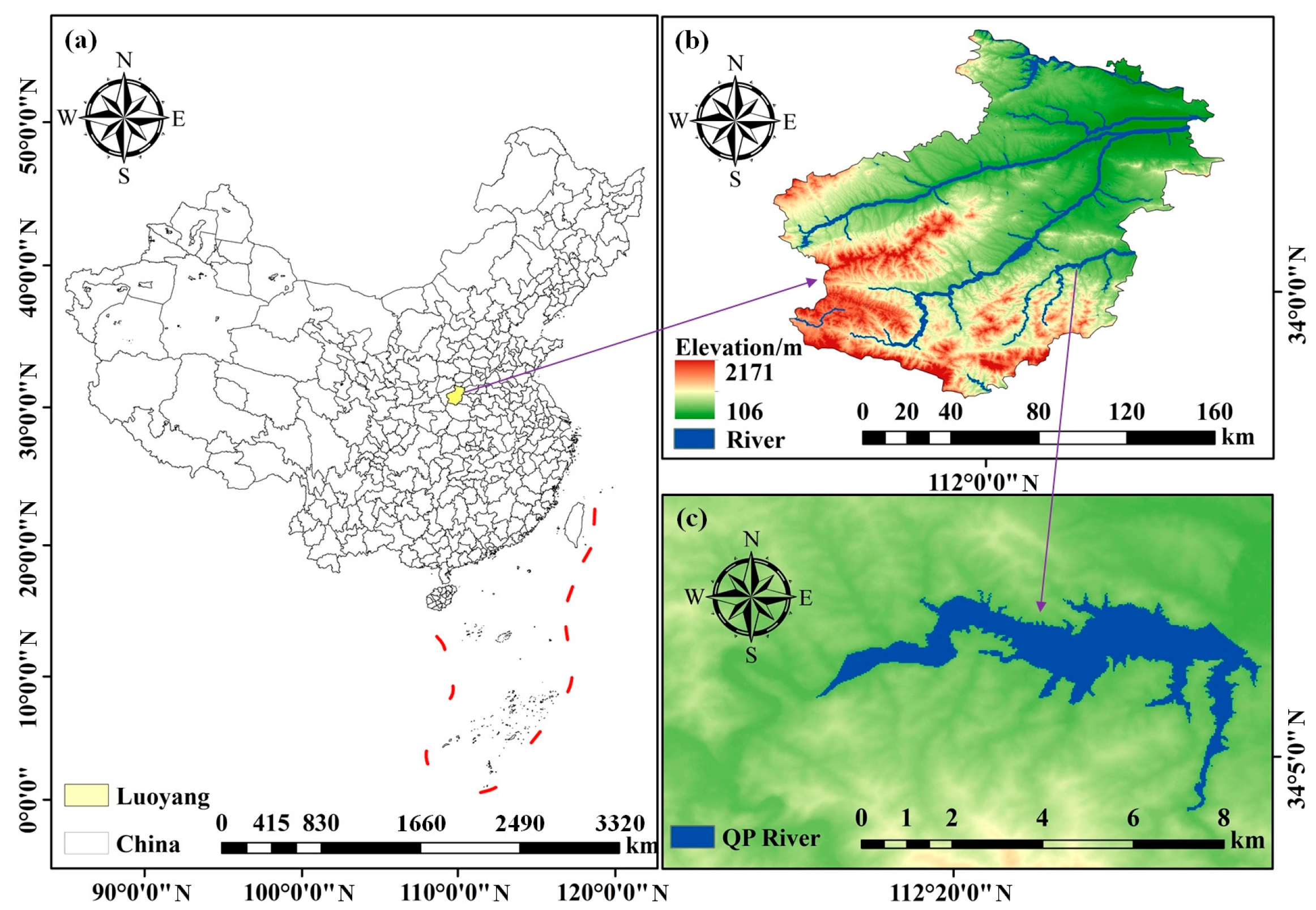
2.1. Data Description
2.2. Extreme-Point Symmetric Mode Decomposition
2.3. Bayesian Decomposition Algorithm
2.4. Cross-Wavelet Transform
2.5. Runoff Prediction Methods
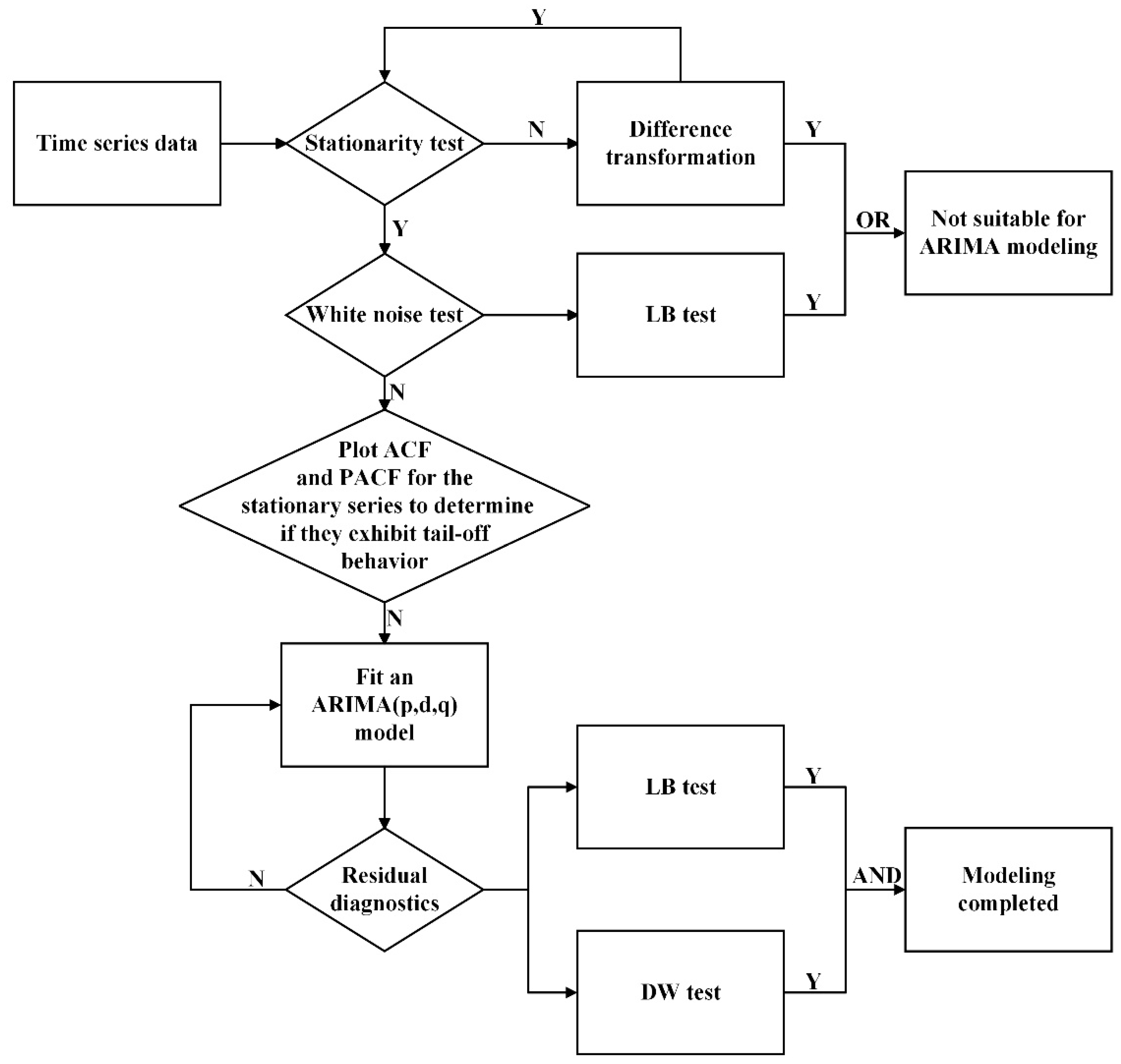
2.5.1. ARIMA Model
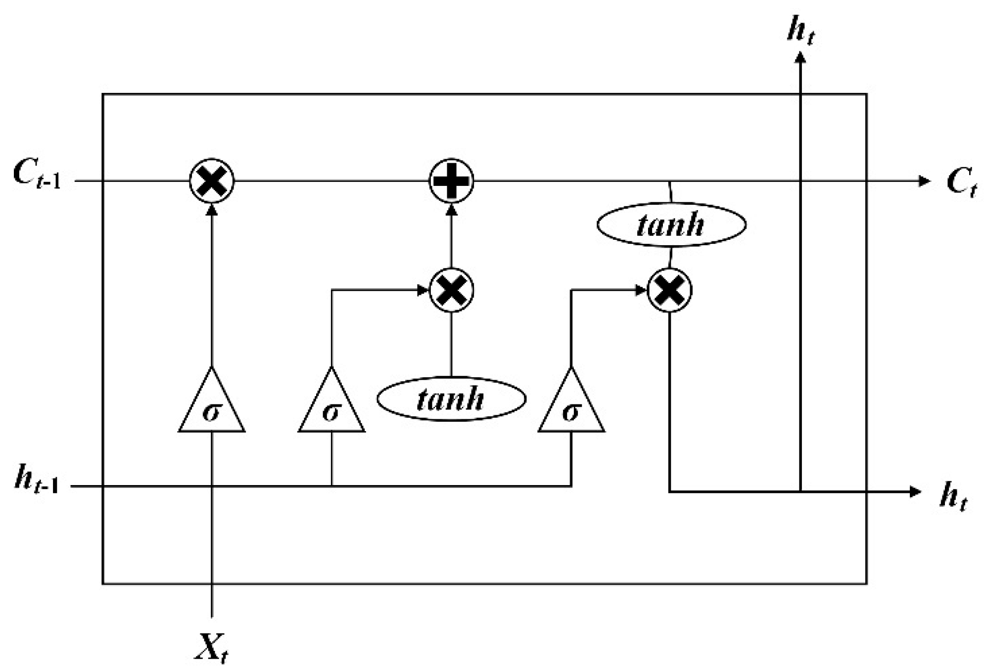
2.5.2. LSTM Model
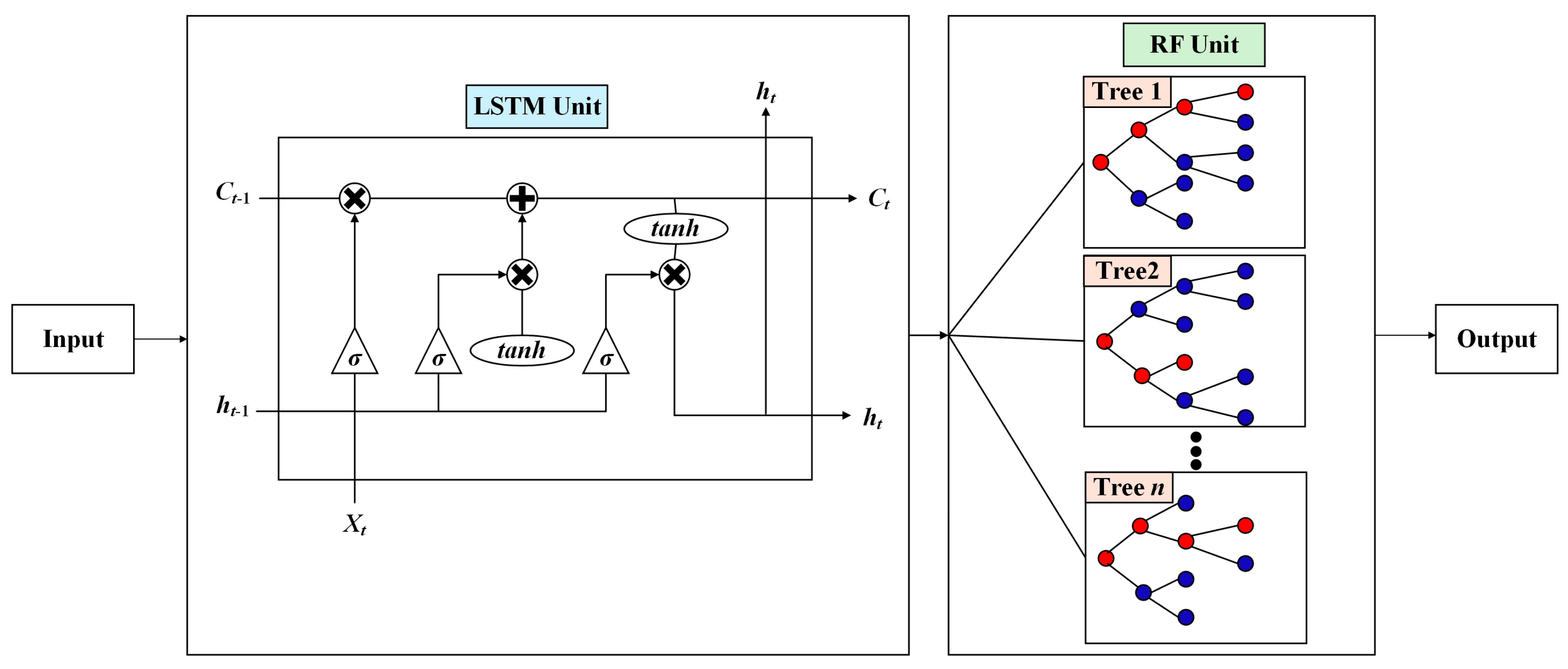
2.5.3. LSTM-RF Model
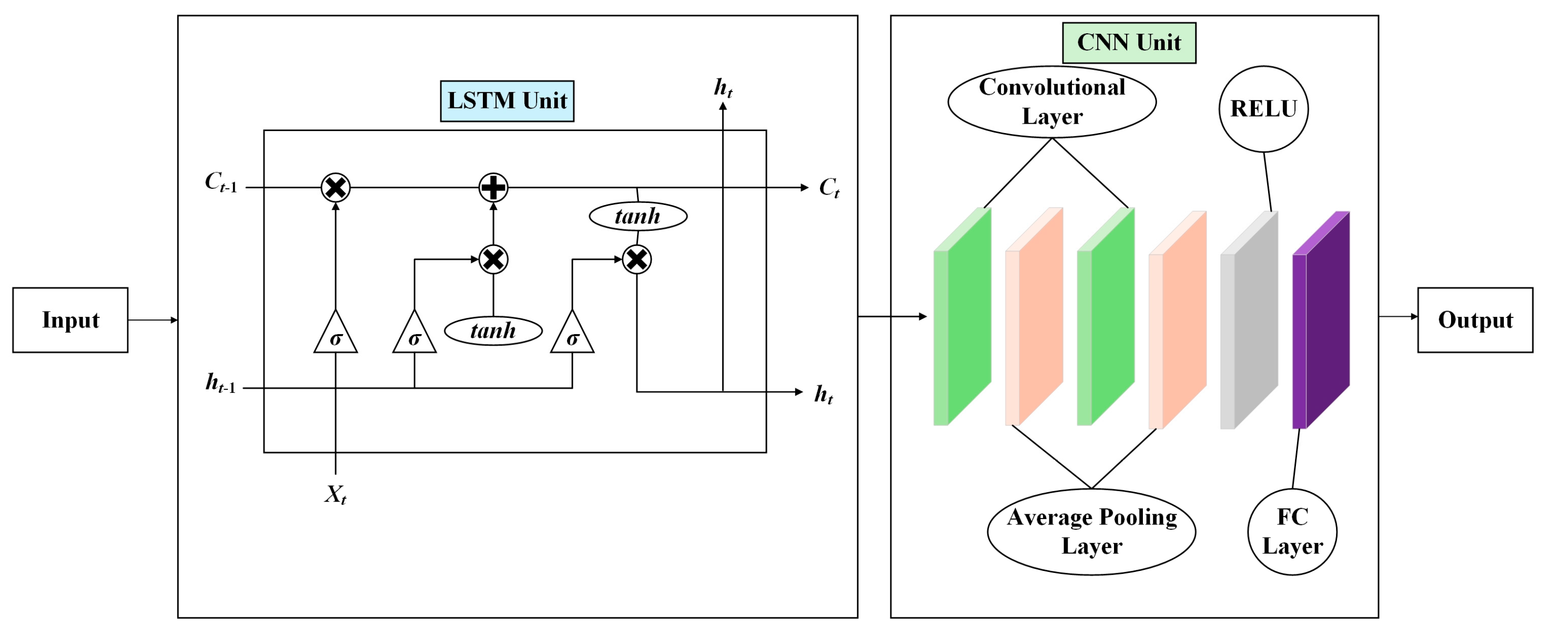
2.5.4. LSTM-CNN Model
3. Results
3.1. Characteristics of Annual Runoff Variation
3.2. Driving Mechanism of Climate Factors on Annual Runoff
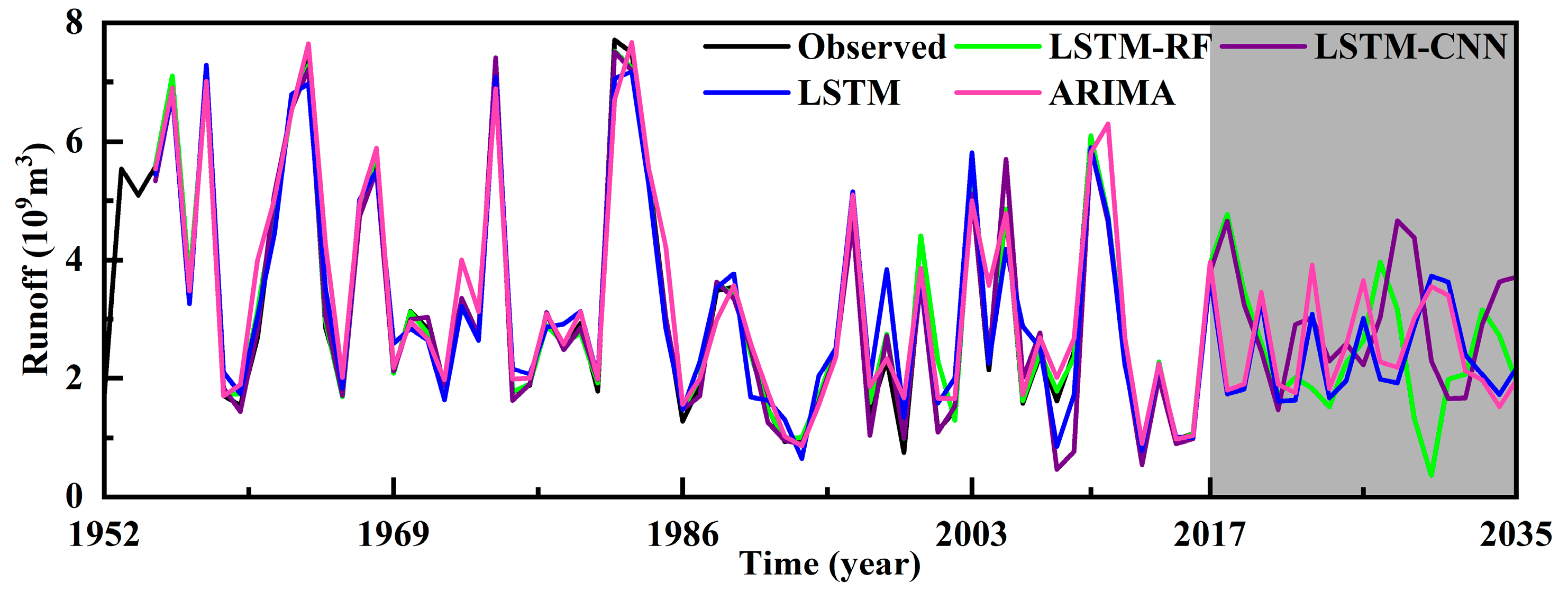
3.3. Future Projections of Annual Runoff Variability in QP Reservoir
4. Discussion
5. Conclusions
- (1)
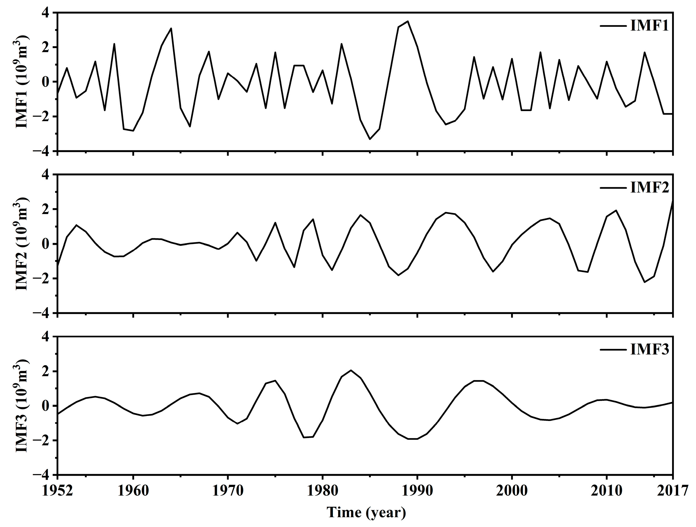
- The annual runoff series of QP Reservoir exhibits quasi-8.25-year short- to medium-term periodic characteristics and quasi-13.20-year long-term periodic characteristics on an interannual scale.
- (2)
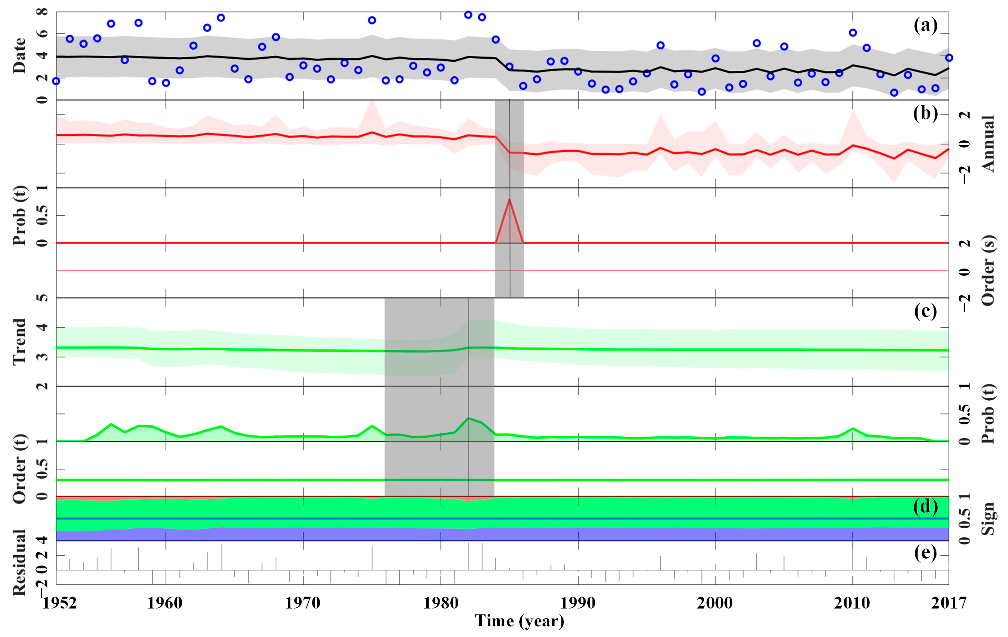
- An annual abrupt change point with a probability of 79.1% was detected in the annual runoff of QP Reservoir in 1985, with a confidence interval spanning from 1984 to 1986.
- (3)
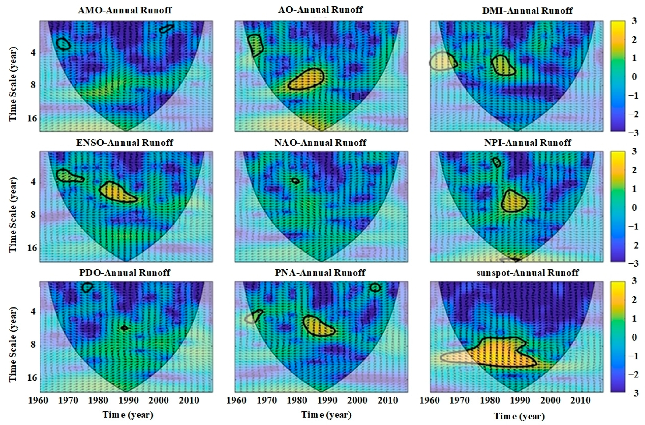
- The periodic correlations between the annual runoff of QP Reservoir and climate drivers vary spatially and temporally: AMO, AO, and PNA exhibit multi-scale synergy; DMI and ENSO show only phase-specific weak coupling; while solar sunspot activity exerts long-term modulation on runoff.
- (4)
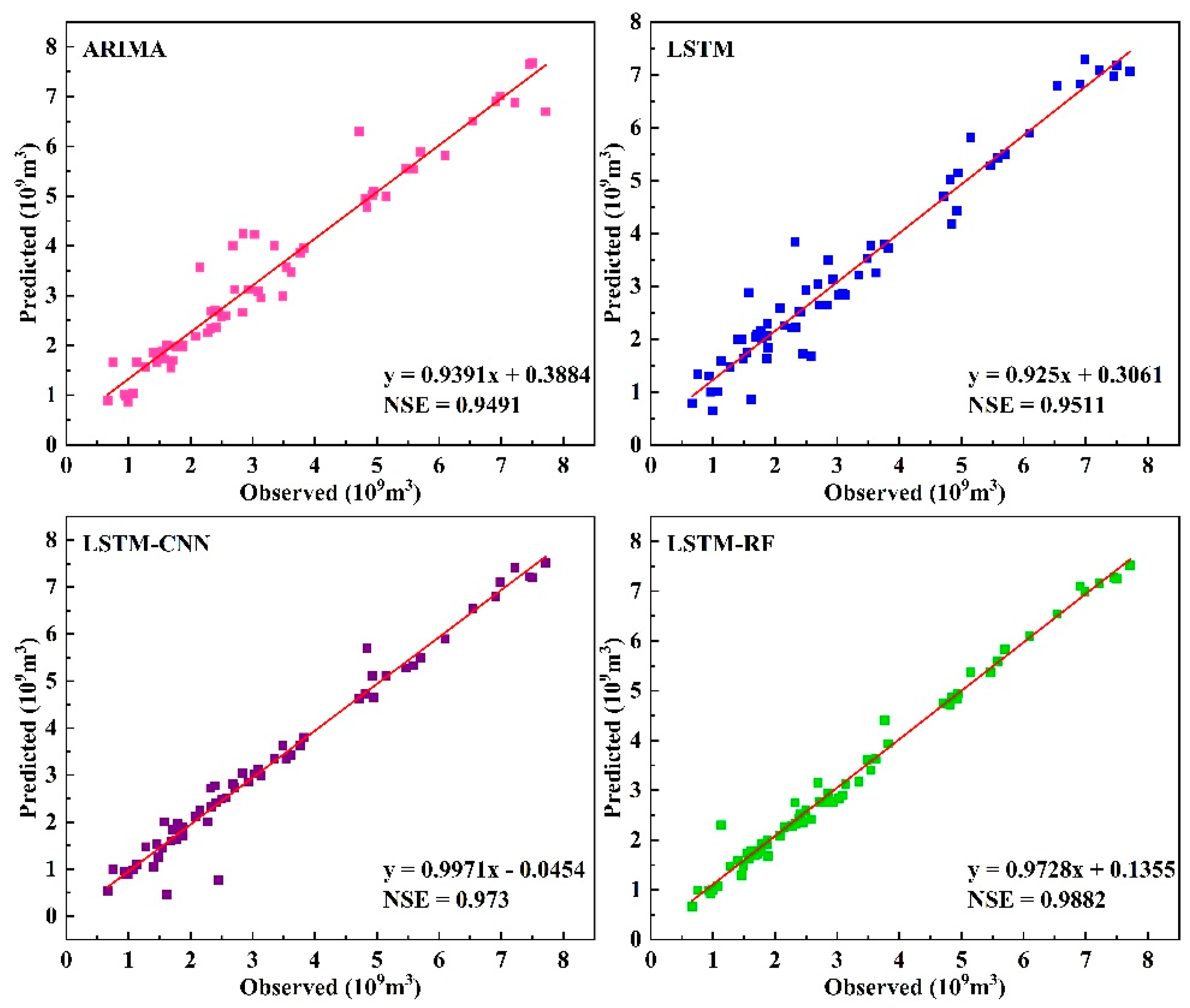
- The NSE of the ARIMA, LSTM, LSTM-RF, and LSTM-CNN models all exceed 0.945, the RMSE is below 0.477 × 10⁹ m3, and the MAE is below 0.297 × 10⁹ m3, Among them, the LSTM-RF model demonstrated the highest accuracy and the most stable predicted fluctuations, indicating that future annual runoff will continue to fluctuate but with a decreasing amplitude.
Author Contributions
Funding
Data Availability Statement
Conflicts of Interest
References
- Xu, E.; Wang, H.; Li, Y.; Dong, N.; Chen, Q.; Tian, H.; Hu, Y.; Tian, G.; Lei, Y.; Li, C.; et al. Analysis of changes and driving forces of landscape pattern vulnerability at Qianping Reservoir in Central China. Environ. Monit. Assess. 2024, 196, 981. [Google Scholar] [CrossRef] [PubMed]
- Yang, F.; Li, C.; Hu, Y.; Tian, G.; Lei, Y.; Wei, D.; Xu, E. Spatial-Temporal Evolution and Prediction of Habitat Quality Before and After the Construction of Qianping Reservoir. Yellow River 2023, 45, 101–107, 147. (In Chinese) [Google Scholar]
- Mo, S.; Yang, J.; Liang, W.; Zhang, G.; Lyu, J. Generalized additive models for design annual runoff and design flood in Jialu River basin. J. Hydroelectr. Eng. 2024, 43, 14–29. (In Chinese) [Google Scholar]
- Zhao, J.; Gao, Y.; Zhang, J.; Li, Y.; Gao, X.; Yuan, H.; Dong, J.; Li, X. Community characteristics of macrobenthos and ecosystem health assessment in ten reservoirs of Henan Province, China. Sci. Rep. 2024, 14, 31531. [Google Scholar] [CrossRef]
- Ni, Y.; Lv, X.; Yu, Z.; Wang, J.; Ma, L.; Zhang, Q. Intra-annual variation in the attribution of runoff evolution in the Yellow River source area. Catena 2023, 225, 107032. [Google Scholar] [CrossRef]
- Lv, C.; Wang, X.; Ling, M.; Xu, W.; Yan, D. Effects of precipitation concentration and human activities on city runoff changes. Water Resour. Manag. 2023, 37, 5023–5036. [Google Scholar] [CrossRef]
- Chen, X.; Li, F.; Wu, F.; Xu, X.; Zhao, Y. Initial water rights allocation of Industry in the Yellow River basin driven by high-quality development. Ecol. Model. 2023, 477, 110272. [Google Scholar] [CrossRef]
- Zhu, M.; Zhang, X.; Elahi, E.; Fan, B.; Khalid, Z. Assessing ecological product values in the Yellow River Basin: Factors, trends, and strategies for sustainable development. Ecol. Indic. 2024, 160, 111708. [Google Scholar] [CrossRef]
- Wang, A.; Wang, S.; Liang, S.; Yang, R.; Yang, M.; Yang, J. Research on ecological protection and high-quality development of the lower Yellow River based on system dynamics. Water 2023, 15, 3046. [Google Scholar] [CrossRef]
- Agbo, E.P.; Nkajoe, U.; Edet, C.O. Comparison of Mann–Kendall and Şen’s innovative trend method for climatic parameters over Nigeria’s climatic zones. Clim. Dyn. 2023, 60, 3385–3401. [Google Scholar] [CrossRef]
- Wu, C.; Xu, R.; Qiu, D.; Ding, Y.; Gao, P.; Mu, X.; Zhao, G. Runoff characteristics and its sensitivity to climate factors in the Weihe River Basin from 2006 to 2018. J. Arid Land 2022, 14, 1344–1360. [Google Scholar] [CrossRef]
- Drogkoula, M.; Kokkinos, K.; Samaras, N. A comprehensive survey of machine learning methodologies with emphasis in water resources management. Appl. Sci. 2023, 13, 12147. [Google Scholar] [CrossRef]
- Wang, W.; Cheng, Q.; Chau, K.; Hu, H.; Zang, H.; Xu, D. An enhanced monthly runoff time series prediction using extreme learning machine optimized by salp swarm algorithm based on time varying filtering based empirical mode decomposition. J. Hydrol. 2023, 620, 129460. [Google Scholar] [CrossRef]
- Liao, S.; Wang, H.; Liu, B.; Ma, X.; Zhou, B.; Su, H. Runoff Forecast Model based on an EEMD-ANN and Meteorological factors using a multicore parallel algorithm. Water Resour. Manag. 2023, 37, 1539–1555. [Google Scholar] [CrossRef]
- Guo, S.; Wen, Y.; Zhang, X.; Chen, H. Runoff prediction of lower Yellow River based on CEEMDAN–LSSVM–GM (1, 1) model. Sci. Rep. 2023, 13, 1511. [Google Scholar] [CrossRef]
- Zhang, X.; Wang, X.; Li, H.; Sun, S.; Liu, F. Monthly runoff prediction based on a coupled VMD-SSA-BiLSTM model. Sci. Rep. 2023, 13, 13149. [Google Scholar] [CrossRef]
- Zhu, S.; Wei, J.; Zhang, H.; Xu, Y.; Qin, H. Spatiotemporal deep learning rainfall-runoff forecasting combined with remote sensing precipitation products in large scale basins. J. Hydrol. 2023, 616, 128727. [Google Scholar] [CrossRef]
- Hu, F.; Yang, Q.; Yang, J.; Luo, Z.; Shao, J.; Wang, G. Incorporating multiple grid-based data in CNN-LSTM hybrid model for daily runoff prediction in the source region of the Yellow River Basin. J. Hydrol. Reg. Stud. 2024, 51, 101652. [Google Scholar] [CrossRef]
- Aderyani, F.R.; Mousavi, S.J.; Jafari, F. Short-term rainfall forecasting using machine learning-based approaches of PSO-SVR, LSTM and CNN. J. Hydrol. 2022, 614, 128463. [Google Scholar] [CrossRef]
- Liu, D.; Chang, Y.; Sun, L.; Wang, Y.; Guo, J.; Xu, L.; Liu, X.; Fan, Z. Multi-Scale Periodic Variations in Soil Moisture in the Desert Steppe Environment of Inner Mongolia, China. Water 2023, 16, 123. [Google Scholar] [CrossRef]
- Han, H.; Jian, H.; Peng, Y.; Yao, S. A conditional copula model to identify the response of runoff probability to climatic factors. Ecol. Indic. 2023, 146, 109415. [Google Scholar] [CrossRef]
- Zhang, S.; Zhu, K.; Wang, C. A Novel Monthly Runoff Prediction Model Based on KVMD and KTCN-LSTM-SA. Water 2025, 17, 460. [Google Scholar] [CrossRef]
- Sun, Z.; Liu, Y.; Zhang, J.; Chen, H.; Shu, Z.; Chen, X.; Jin, J.; Liu, C.; Bao, Z.; Wang, G. Research progress and prospect of mid-long term runoff prediction. Water Resour. Prot. 2023, 39, 136–144. [Google Scholar]
- Lotfipoor, A.; Patidar, S.; Jenkins, D.P. Deep neural network with empirical mode decomposition and Bayesian optimisation for residential load forecasting. Expert Syst. Appl. 2024, 237, 121355. [Google Scholar] [CrossRef]
- Wu, L.; Chen, D.; Yang, D.; Luo, G.; Wang, J.; Chen, F. Response of runoff change to extreme climate evolution in a typical watershed of Karst trough valley, SW China. Atmosphere 2023, 14, 927. [Google Scholar] [CrossRef]
- Wang, F.; Men, R.; Yan, S.; Wang, Z.; Lai, H.; Feng, K.; Gao, S.; Li, Y.; Guo, W.; Tian, Q. Identification of the Runoff Evolutions and Driving Forces during the Dry Season in the Xijiang River Basin. Water 2024, 16, 2317. [Google Scholar] [CrossRef]
- Cui, A.; Li, J.; Zhou, Q.; Zhu, H.; Liu, H.; Yang, C.; Wu, G.; Li, Q. Propagation Dynamics from Meteorological Drought to GRACE-Based Hydrological Drought and Its Influencing Factors. Remote Sens. 2024, 16, 976. [Google Scholar] [CrossRef]
- Guo, J.; Liu, Y.; Zou, Q.; Ye, L.; Zhu, S.; Zhang, H. Study on optimization and combination strategy of multiple daily runoff prediction models coupled with physical mechanism and LSTM. J. Hydrol. 2023, 624, 129969. [Google Scholar] [CrossRef]
- Yao, Z.; Wang, Z.; Wang, D.; Wu, J.; Chen, L. An ensemble CNN-LSTM and GRU adaptive weighting model based improved sparrow search algorithm for predicting runoff using historical meteorological and runoff data as input. J. Hydrol. 2023, 625, 129977. [Google Scholar] [CrossRef]
- Bian, L.; Qin, X.; Zhang, C.; Guo, P.; Wu, H. Application, interpretability and prediction of machine learning method combined with LSTM and LightGBM-a case study for runoff simulation in an arid area. J. Hydrol. 2023, 625, 130091. [Google Scholar] [CrossRef]
- Chen, Z.; Lin, H.; Shen, G. TreeLSTM: A spatiotemporal machine learning model for rainfall-runoff estimation. J. Hydrol. Reg. Stud. 2023, 48, 101474. [Google Scholar] [CrossRef]
- Xu, W.; Chen, J.; Zhang, X.J. Scale effects of the monthly streamflow prediction using a state-of-the-art deep learning model. Water Resour. Manag. 2022, 36, 3609–3625. [Google Scholar] [CrossRef]
- Huang, S.; Yu, L.; Luo, W.; Pan, H.; Li, Y.; Zou, Z.; Wang, W.; Chen, J. Runoff prediction of irrigated paddy areas in Southern China based on EEMD-LSTM model. Water 2023, 15, 1704. [Google Scholar] [CrossRef]
- Xue, H.; Guo, C.; Dong, G.; Zhang, C.; Lian, Y.; Yuan, Q. Prediction of runoff in the upper reaches of the Hei River based on the LSTM model guided by physical mechanisms. J. Hydrol. Reg. Stud. 2025, 58, 102218. [Google Scholar] [CrossRef]
- Samantaray, S.; Sahoo, A.; Satapathy, D.P.; Oudah, A.; Yaseen, Z. Suspended sediment load prediction using sparrow search algorithm-based support vector machine model. Sci. Rep. 2024, 14, 12889. [Google Scholar] [CrossRef]
- Gleick, P.H. Roadmap for sustainable water resources in southwestern North America. Proc. Natl. Acad. Sci. USA 2010, 107, 21300–21305. [Google Scholar] [CrossRef]
- Liu, J.; Song, T.; Mei, C.; Wang, H.; Zhang, D.; Nazli, S. Flood risk zoning of cascade reservoir dam break based on a 1D-2D coupled hydrodynamic model: A case study on the Jinsha-Yalong River. J. Hydrol. 2024, 639, 131555. [Google Scholar] [CrossRef]
- Shen, X.; Wu, X.; Xie, X.; Wei, C.; Li, L.; Zhang, J. Synergetic theory-based water resource allocation model. Water Resour. Manag. 2021, 35, 2053–2078. [Google Scholar] [CrossRef]
- Li, Z.; Zhang, X. A novel coupled model for Monthly Rainfall Prediction based on ESMD-EWT-SVD-LSTM. Water Resour. Manag. 2024, 38, 3297–3312. [Google Scholar] [CrossRef]
- Wei, C.; Du, Z.; Zhou, M.; Zhang, M.; Sun, Y.; Liu, Y. Spatiotemporal analysis of groundwater storage variations based on extreme-point symmetric mode decomposition and independent component analysis in Murray-Darling Basin, Australia. Hydrogeol. J. 2023, 31, 967–983. [Google Scholar] [CrossRef]
- Sattari, A.; Jafarzadegan, K.; Moradkhani, H. Enhancing streamflow predictions with machine learning and Copula-Embedded Bayesian model averaging. J. Hydrol. 2024, 643, 131986. [Google Scholar] [CrossRef]
- Zhang, M.; Zhang, X.; Qiao, W.; Lu, Y.; Chen, H. Forecasting of runoff in the lower Yellow River based on the CEEMDAN–ARIMA model. Water Supply 2023, 23, 1434–1450. [Google Scholar] [CrossRef]
- Khaldi, R.; El Afia, A.; Chiheb, R.; Tabik, S. What is the best RNN-cell structure to forecast each time series behavior? Expert Syst. Appl. 2023, 215, 119140. [Google Scholar] [CrossRef]
- Guo, S.; Sun, S.; Zhang, X.; Chen, H.; Li, H. Monthly precipitation prediction based on the EMD–VMD–LSTM coupled model. J. Water Supply 2023, 23, 4742–4758. [Google Scholar] [CrossRef]
- Park, S.; Kim, J.; Kang, J. Heuristic approach to urban sewershed delineation for pluvial flood modeling. J. Water Process Eng. 2024, 67, 106129. [Google Scholar] [CrossRef]
- Ji, J.; Sun, M.; Ji, G.; Li, L.; Chen, W.; Huang, J.; Guo, Y. Simulation of actual evaporation and its multi-time scale attribution analysis for major rivers in China. J. Hydrol. 2025, 657, 133121. [Google Scholar] [CrossRef]
- Goda, T.; Kazashi, Y.; Suzuki, Y. Randomizing the trapezoidal rule gives the optimal RMSE rate in Gaussian Sobolev spaces. Math. Comput. 2024, 93, 1655–1676. [Google Scholar] [CrossRef]
- Robeson, S.M.; Willmott, C.J. Decomposition of the mean absolute error (MAE) into systematic and unsystematic components. PLoS ONE 2023, 18, e0279774. [Google Scholar] [CrossRef]
- Yin, H.; Zhu, W.; Zhang, X.; Xing, Y.; Xia, R.; Liu, J.; Zhang, Y. Runoff predictions in new-gauged basins using two transformer-based models. J. Hydrol. 2023, 622, 129684. [Google Scholar] [CrossRef]
- Wang, B.; Wang, H.; Jiao, X.; Huang, L.; Chen, H.; Guo, W. Runoff change in the Yellow River Basin of China from 1960 to 2020 and its driving factors. J. Arid Land 2024, 16, 168–194. [Google Scholar] [CrossRef]
- Kuang, X.; Liu, J.; Scanlon, B.R.; Jiao, J.; Jasechko, S.; Lancia, M.; Biskaborn, B.; Wada, Y.; Li, H.; Zeng, Z.; et al. The changing nature of groundwater in the global water cycle. Science 2024, 383, eadf0630. [Google Scholar] [CrossRef]
- Zhang, J.; Guan, Q.; Zhang, Z.; Shao, W.; Zhang, E.; Kang, T.; Xiao, X.; Liu, H.; Luo, H. Characteristics of spatial and temporal dynamics of vegetation and its response to climate extremes in ecologically fragile and climate change sensitive areas–a case study of Hexi region. Catena 2024, 239, 107910. [Google Scholar] [CrossRef]
- Ji, J.; Wang, T.; Liu, J.; Wang, M.; Tang, W. River runoff causal discovery with deep reinforcement learning. Appl. Intell. 2024, 54, 3547–3565. [Google Scholar] [CrossRef]
- Qian, L.; Hu, W.; Zhao, Y.; Hong, M.; Fan, L. A coupled model of nonlinear dynamical system and deep learning for multi-step ahead daily runoff prediction for data scarce regions. J. Hydrol. 2025, 653, 132640. [Google Scholar] [CrossRef]


| IMF Component | IMF1 | IMF2 | IMF3 | R |
|---|---|---|---|---|
| Period (Year) | 8.25 | 9.14 | 13.20 | |
| Variance Contribution Rate (%) | 48.17 | 20.56 | 14.61 | 16.66 |
| Correlation Coefficient | 0.58 | 0.27 | 0.34 | 0.42 |
| Model Name | RMSE (109 m3) | MAE (109 m3) | NSE |
|---|---|---|---|
| ARIMA | 0.477 | 0.297 | 0.949 |
| LSTM | 0.437 | 0.331 | 0.951 |
| LSTM-CNN | 0.3272 | 0.192 | 0.973 |
| LSTM-RF | 0.219 | 0.129 | 0.988 |
Disclaimer/Publisher’s Note: The statements, opinions and data contained in all publications are solely those of the individual author(s) and contributor(s) and not of MDPI and/or the editor(s). MDPI and/or the editor(s) disclaim responsibility for any injury to people or property resulting from any ideas, methods, instructions or products referred to in the content. |
© 2025 by the authors. Licensee MDPI, Basel, Switzerland. This article is an open access article distributed under the terms and conditions of the Creative Commons Attribution (CC BY) license (https://creativecommons.org/licenses/by/4.0/).
Share and Cite
Kang, X.; Yu, H.; Yang, C.; Tian, Q.; Wang, Y. Analysis of Evolutionary Characteristics and Prediction of Annual Runoff in Qianping Reservoir. Water 2025, 17, 1902. https://doi.org/10.3390/w17131902
Kang X, Yu H, Yang C, Tian Q, Wang Y. Analysis of Evolutionary Characteristics and Prediction of Annual Runoff in Qianping Reservoir. Water. 2025; 17(13):1902. https://doi.org/10.3390/w17131902
Chicago/Turabian StyleKang, Xiaolong, Haoming Yu, Chaoqiang Yang, Qingqing Tian, and Yadi Wang. 2025. "Analysis of Evolutionary Characteristics and Prediction of Annual Runoff in Qianping Reservoir" Water 17, no. 13: 1902. https://doi.org/10.3390/w17131902
APA StyleKang, X., Yu, H., Yang, C., Tian, Q., & Wang, Y. (2025). Analysis of Evolutionary Characteristics and Prediction of Annual Runoff in Qianping Reservoir. Water, 17(13), 1902. https://doi.org/10.3390/w17131902