Article

Temporal Hydrological Responses to Progressive Land Cover Changes and Climate Trends in a Plateau Lake Basin in Southwest China

by
Zhengduo Bao
1,2,*,
Yuxuan Wu
3,4,
Weining He
3,4,
Nian She
1,5,
Hua Shao
6 and
Chao Fan
7
1
Tsinghua Innovation Center in Zhuhai, Zhuhai 519000, China
2
School of Resource and Environmental Sciences, Wuhan University, Wuhan 430072, China
3
Hunan Engineering Research Center of Sponge City Construction Integration Technology, Changsha 410004, China
4
China Machinery International Engineering Design and Research Institute Co., Ltd., Changsha 410004, China
5
School of Human Settlements and Civil Engineering, Xi’an Jiaotong University, Xi’an 710049, China
6
Urban Management Bureau of Yinchuan City, Yinchuan 750001, China
7
Bejing Planning and Design Consultants Ltd., China Academy of Urban Planning and Design, Beijing 100044, China
*
Author to whom correspondence should be addressed.
Water 2025, 17(13), 1890; https://doi.org/10.3390/w17131890
Submission received: 8 May 2025 / Revised: 18 June 2025 / Accepted: 24 June 2025 / Published: 25 June 2025

Abstract

The reducing streamflow is a major concern in the Yilong Lake Basin (YLB), which supplies water for agriculture and the growing population in the basin and to maintain the health of the regional ecosystem. The YLB has experienced remarkable land use/land cover change (LUCC) and climate change (CC) in recent years. To understand the drivers of the streamflow change in this basin, the effects of the land use change and climate variation on the temporal flow variability were studied using the Soil and Water Assessment Tool (SWAT). The calibration and validation results indicated that the SWAT simulated the streamflow well. Then the streamflow responses to the land use change between 2010 and 2020 and climate change with future climate projections (SSP245, SSP370, and SSP585) were evaluated. Results showed that the LUCC in the YLB caused a marginal decline in the annual streamflow at the whole basin scale but significantly altered rainfall–runoff relationships and intra-annual discharge patterns; e.g., monthly streamflows decreased by up to 3% in the dry season under the surface modification, with subbasins of the YLB exhibiting divergent responses attributed to spatial heterogeneity in land surface transitions. Under future climate scenarios, streamflow projections revealed general declining trends with significant uncertainties, particularly under high-emission pathways, e.g., SSP370 and SSP585, in which the streamflow could be projected to reduce by up to 5.9% in the mid-future (2031–2045). In addition, droughts were expected to intensify, exacerbating seasonal water stress in the future. It suggests that integrated water governance should synergize climate-resilient land use policies with adaptive infrastructure to address regional water resources challenges.

1. Introduction

Watersheds are critical environmental units of terrestrial ecosystems, sustaining essential ecosystem services, including the water supply, biodiversity conservation, and flood regulation [1,2]. As fundamental to watershed ecosystem functioning, hydrological processes are regulated by complex interactions among natural factors, e.g., topography, precipitation, vegetation, and anthropogenic activities [3,4,5]. In some regions, human-induced land surface modifications can dramatically alter water cycle processes, such as infiltration and evapotranspiration [6,7], thereby reshaping watershed hydrological regimes [8,9]. For example, Fang et al. [10] showed that converting a rice paddy field to an urban use directly reduced ET in Qinghuai River Basin. Studies demonstrated that the urbanization, leading to an expansion of impermeable surfaces, has caused sharp increases in the streamflow at both long-term and short-term scales [11,12,13]. Alongside these anthropogenic factors, climate change (CC) further exacerbates the hydrological variability in watersheds by altering the amount and intensity of meteorological factors like precipitation and temperature [14]. Regional averaged surface mean temperatures in Southwest China (SWC) are projected to increase by 1.50–2.17 °C during 2041–2060 under different climate scenarios [15], and droughts in SWC are predicted to become more frequent and extreme under continued global warming [14].
Previous studies have identified land use/land cover change (LUCC) and CC as the primary drivers of hydrological dynamics in diverse regions [16,17,18]. The impacts of climate and LUCC on streamflow exhibit spatial distinctiveness [19]. For example, Zhou et al. [20] estimated that streamflow declined from 6% to 21% in response to CC in the watershed of Lake Dianchi, Yunnan’s largest plateau lake. Duan et al. [21] found that Lake Dianchi’s watershed hydrological regimes were more sensitive to precipitation than air temperature. Zhang et al. [22] demonstrated that increased temperature and decreased rainfall caused a 39.1% streamflow decline, while LUCC induced a 2.2–3.9% increase in the Loess plateau. Lu et al. [16] evaluated that the land use changes contributed to 17–30% of the runoff depth variation in China’s Songnen Plain.
Combined climate–hydrological modeling systems integrating a LUCC and CC consideration serve as effective tools for assessing their impacts on watershed water resources and hydrology [19,23]. For climate projection, outputs from global climate models (GCMs) are typically used to predict CC in the future. However, GCMs have a low resolution (100–300 km), which is inadequate for small- to medium-scale studies [24]. Thus, GCM data are often downscaled using statistical, dynamic, or other methods [25,26]. The Coupled Model Intercomparison Project Phase 6 (CMIP6) provides the latest multi-GCM output datasets [27]. For hydrologic simulations, numerous models, such as the Variable Infiltration Capacity (VIC) [28], Soil and Water Assessment Tool (SWAT) [29,30], MIKE SHE [31], and Coupled Groundwater and Surface Water Flow Model (GSFLOW) [32], have been widely applied to simulate streamflow and evaluate the impacts of human disturbances and climate variation on watershed hydrology [32,33].
Yilong Lake is one of the nine largest plateau lakes in Yunnan Province and an important migrate channel for birds, representing a typical wetland resource type in the Yunnan–Guizhou Plateau. With a fragile karst landscape, the hydrological processes of the Yilong Lake Basin (YLB) are extremely vulnerable to human activities (e.g., land use change) and climate variation. Over recent decades, extensive land surface modification (e.g., urbanization) has caused severe ecological degradation [34,35], while CC projections indicate an increasing drought frequency and intensity [36,37]. Understanding hydrological responses to LUCC and CC is critical for regional sustainable water resource management and watershed development policy. Therefore, this research aims to (1) characterize the land use transition in the YLB during 2010–2020; (2) evaluate streamflow changes under 2010 and 2020 land use conditions over the historical period (1980–2020); (3) project streamflow trends in the YLB under different SSP scenarios for 2015–2060, thereby providing a scientific basis for the YLB’s water resource management, sustainable development, and regional governance.

2. Materials and Methods

2.1. Study Area

Yilong Lake Basin is located in Shiping County, south–central of Yunnan (23°36′–23°48′ N, 102°20′–102°41′ E, shown in Figure 1), covering a total area of 360.4 km2 and having an average elevation of 1414 m a.s.l. The basin has six main inflowing streams, namely Chengbei River (CBR), Cheng River (CR), Chengnan River (CNR), Dashui River (DSR), Longgang River (LGR), and Yucun River (YCR), respectively, and one outlet, being Xinjiehai River (XJHR). Based on spatial topography heterogeneity, the land of YLB is divided into nine subbasins: CH (32.39 km2), CBH (89.83 km2), CNH (20.16 km2), DSH (20.16 km2), BASP (26.04 km2), NASP (37.82 km2), LGH (37.72 km2), YCH (11.42 km2), and XJHH (7.61 km2). The regional climate is subtropical monsoon, with distinct dry (November–June) and wet (July–October) seasons. Annual average precipitation, evapotranspiration, and air temperature in the basin are 928.3 mm, 1908.6 mm, and 18 °C, respectively. In addition, the YLB soil types include Dystric Cambisols, Cumulic Anthrosols, Haplic Acrisols, and Humic Acrisols. And the basin encompasses seven major landscape types, including forest (FR), farmland (FL), garden land (GL), grassland (GR), water (WR), urban land (UL), and unused land (UU).
Yilong Lake serves as a crucial stopover for migratory birds, a typical southern Yunnan wetland resource, and a primary water source for the Pearl River as well as for neighboring Shiping and Jianshui counties. As a semi-enclosed watershed, the basin relies on rainfall for local livelihoods and the economy. YLB has experienced dramatic climatic shifts, such as rising temperatures and decreasing precipitation [38]. Over recent decades, the basin has faced severe water resource challenges, most notably when the lake’s water level plummeted to its lowest recorded point in 2013 after a prolonged regional drought starting in 2009 [39]. Meanwhile, since 1980, the basin has undergone obvious land surface modification, including urban expansion, agricultural operation, and reforestation [40]. Inadequate environmental protection, combined with rapid economic development, population growth, urbanization and human activities, continuously affects the hydrology and ecosystem of the basin [41].

2.2. Data and Data Processing

2.2.1. Geospatial Data

The data of digital elevation model (DEM) raster, land use/land cover (LULC), water system shape file, and soil raster covering the study area were obtained from various sources.
Specifically, high-resolution DEM (2.5 m resolution), LULC data, and water system shape file covering the basin were obtained from the Yunnan Geological Data Center with permission. LULC data for 2010 and 2020 were derived from the second and third national land resource surveys, respectively. The original LULC data of YLB, which included 10 primary and 26 secondary land use types, was reclassified into 25 SWAT-supported land use types (shown in Table 1) using the Reclassify module in the ArcGIS Toolbox.
The soil data was sourced from the Chinese Soil Dataset, which is based on the World Soil Database (HWSD) version 1.1. The soil dataset includes a series of soil physical and chemical parameters, e.g., soil type, texture, moisture content, particle size, and composition.

2.2.2. Climate Data

Historical climate data, including daily rainfall; daily average relative humidity; daily average vapor pressure; and daily average, maximum, and minimum temperatures from 1990 to 2020 at the Shiping Meteorological Ground Station, were obtained from Meteorological Bureau of Shiping County with permission. Monthly average solar radiation data were generated using the WXGEN tool in SWAT.
Future climate data were collected from the NASA Earth Exchange Global Daily Downscaled Projections (NEX-GDDP-CMIP6) dataset [42]. The NEX-GDDP-CMIP6 dataset comprises global climate scenarios derived from the GCM runs conducted under the CMIP6 and across the four “Tier 1” greenhouse gas emissions scenarios [42]. The Bias-Correction Spatial Disaggregation (BCSD) method [43], a statistical downscaling algorithm specifically developed to address the limitations of global GCM outputs, was used to generate the NEX-GDDP-CMIP6 dataset.
The NEX-GDDP-CMIP6 provides high-resolution (0.25° × 0.25°), bias-corrected climate projections, including daily time series of humidity; rainfall; wind speed; and average, maximum, and minimum temperature, derived from 35 GCMs in CMIP6 across four scenarios of Shared Socioeconomic Pathways (SSPs)—SSP126, SSP245, SSP370, and SSP585—for 2015–2100 and historical data for 1950–2014. Studies have demonstrated that the dataset effectively reproduces key meteorological parameters, such as daily maximum temperature and rainfall [44,45]. In this study, we utilized downscaled data from four widely used GCMs, such as ACCESS-CM2, ACCESS-ESM1.5, BCC-CSM2-MR, and NorESM2-LM, spanning a reference period (2000–2014) and a projection period (2015–2060). Information about the GCMs is summarized in Table 2. These datasets are associated with three SSP scenarios (SSP245, SSP370, and SSP585) representing a spectrum of CC pathways from relatively sustainable to high emissions.
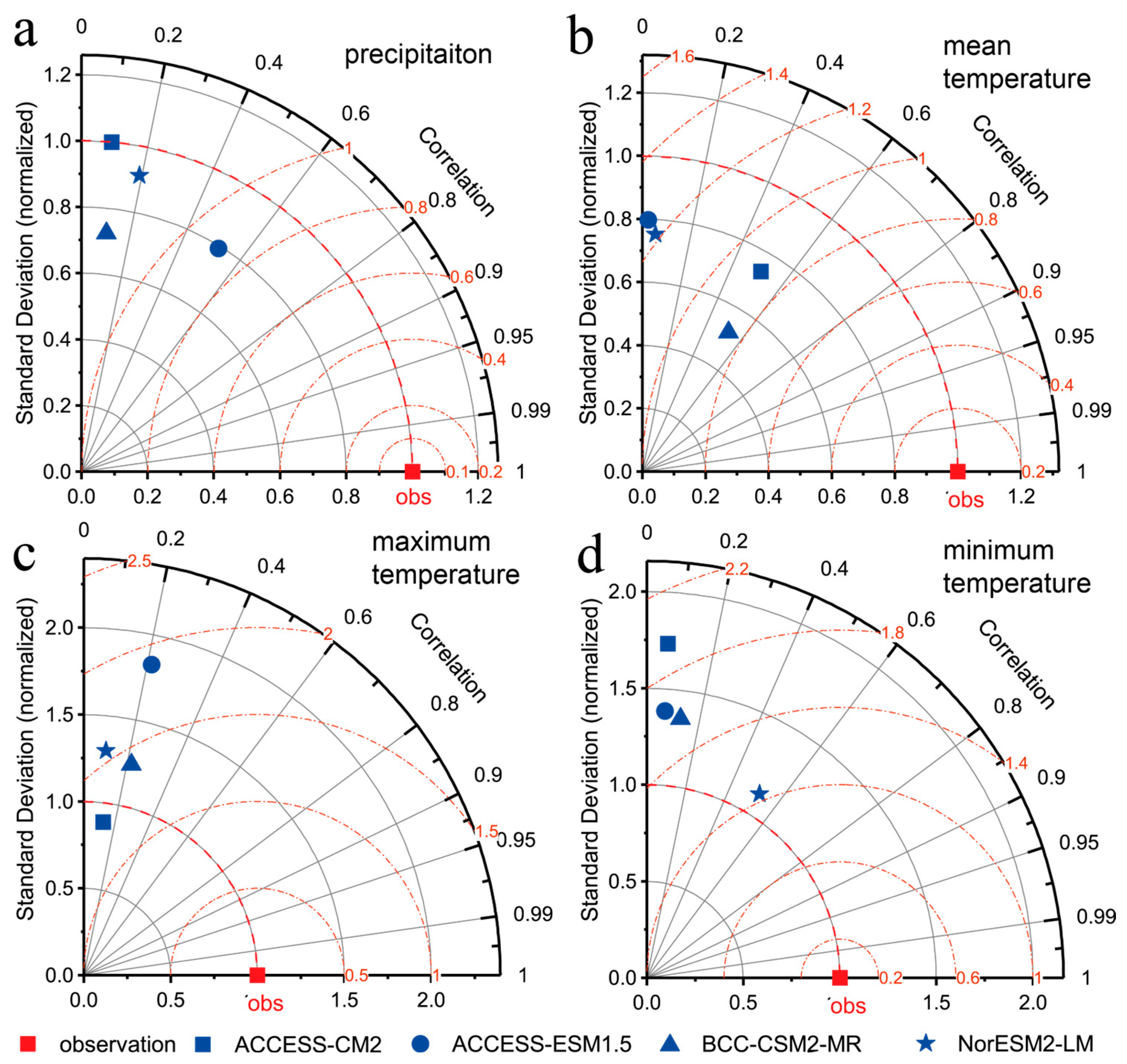
Considering the bias in GCMs’ outputs of NEX-GDDP-CMIP6 dataset for the study area, the downscaled dataset was bias-corrected following quantile mapping method descried in [46] for use in this study. The bias-correction was performed in Python 3.12 using the bias-correction package (https://github.com/pankajkarman/bias_correction, accessed on 20 June 2024). The results, obtained by comparing observed data from the Meteorological Station with the four GCMs during 2000–2014 from NEX-GDDP-CMIP6, are presented in the Taylor diagram (Figure 2). The normalized standard deviation of daily precipitation, daily average temperature, daily maximum temperature, and daily minimum temperature range from 0.76 to 1.0, 0.5 to 0.8, 0.8 to 1.8, and 1.1 to 1.75 for the GCMs. The correlation between observation and GCM outputs varies from 0.03 to 0.57 depending on the GCM and parameter.

2.2.3. Streamflow Data

Monthly streamflow observation data from 2009 to 2018 at the CR hydrologic gauge station were collected from the local water authority with permission.
The description and source of the data in this study are summarized in Table 3.

2.3. Methodology

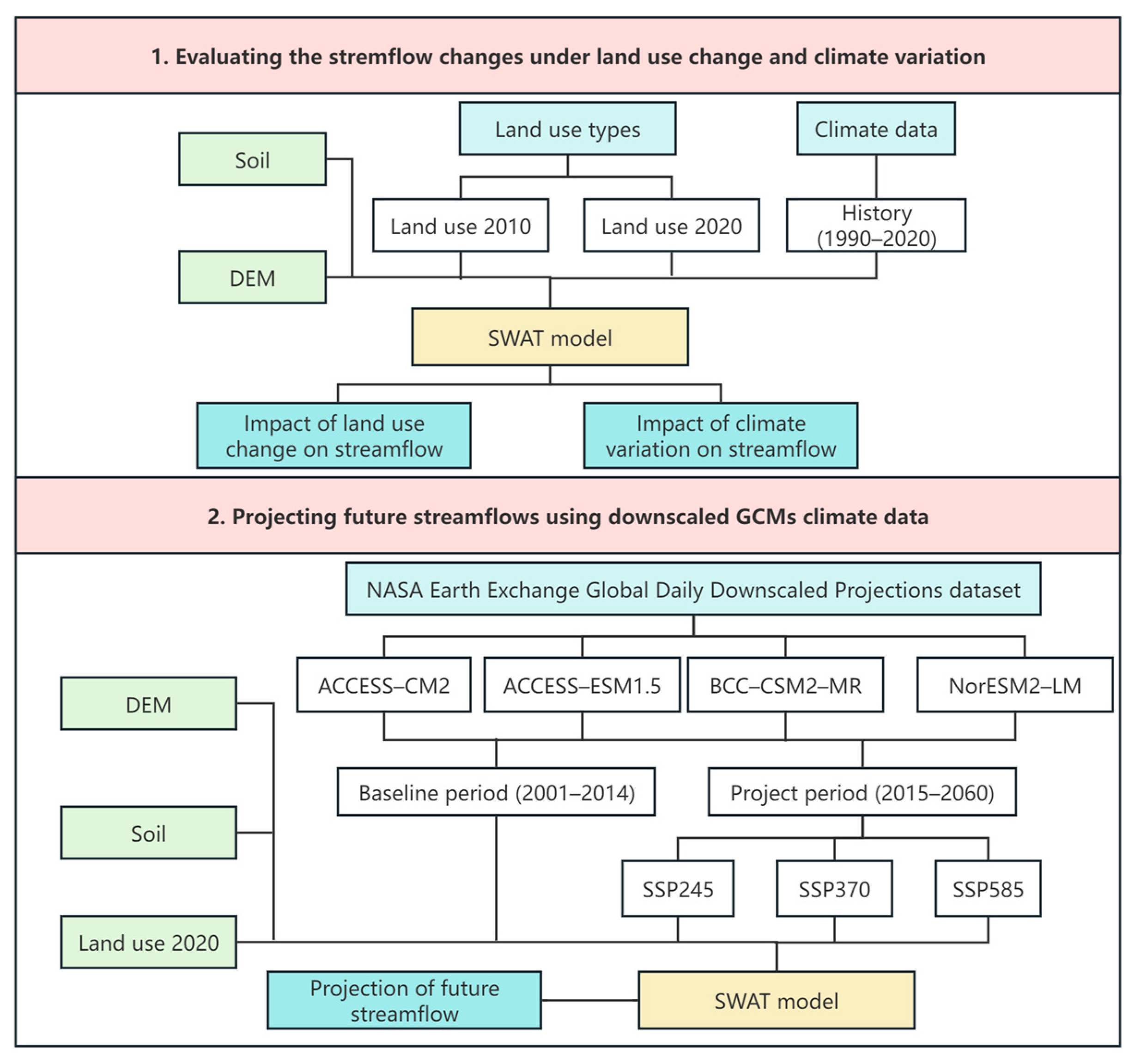
The research framework proposed in this study includes two main components, as shown in Figure 3. First, we estimated the watershed hydrology processes using the SWAT model under two land use scenarios, i.e., LU2010 and LU2020, over the period of 1990–2020, driven by historical local climate data. We assessed the impacts of LUCC and climate variation on the basin streamflow changes, respectively. Second, we evaluated future streamflows for 2015–2060 driven by downscaled future climate scenarios (SSP245, SSP370, and SSP585) from four GCMs obtained from the NEX-GDDP-CMIP6 dataset.
To assess watershed hydrology under different LULC and CC conditions, the DEM, stream network, and soil raster were kept constant in the SWAT model, while land use raster and climate data were replaced accordingly.

2.3.1. Model Description and Setup

SWAT is a basin-scale, semi-physically based, spatially distributed hydrologic model designed to predict the impacts of CC and land management on water, sediment, and nutrient yields in watersheds [47]. The model divides a basin into subcatchments and further into hydrologic response units (HRUs), which are homogeneous areas defined by soil, land cover, and management practices. Detailed description and operation of SWAT can be found in previous documents [47].
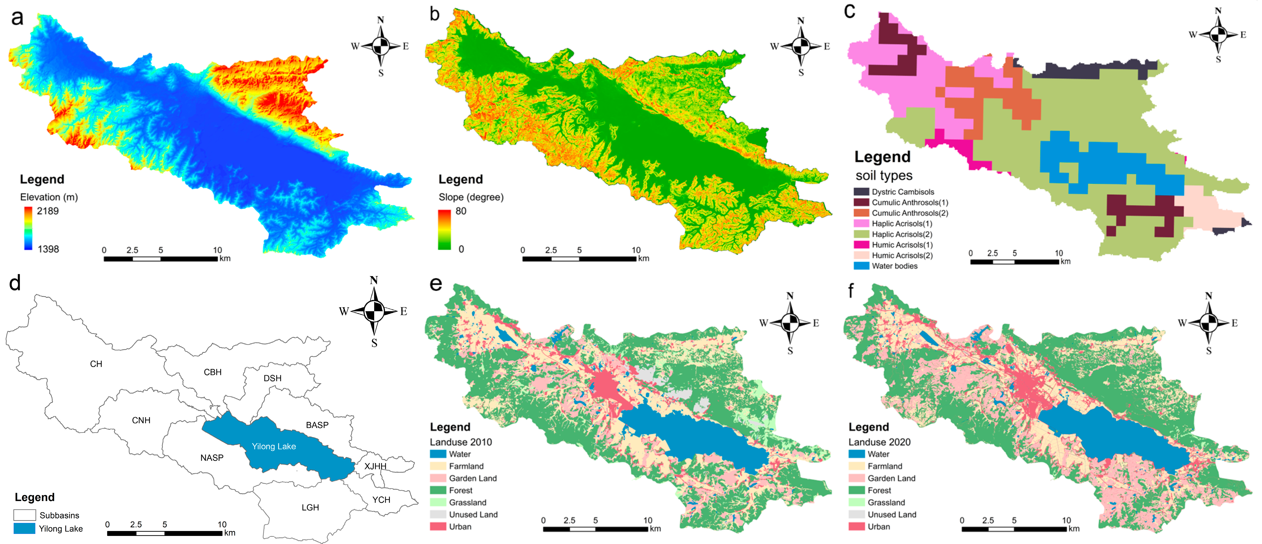
SWAT has been successfully employed to simulate the watershed hydrology in Southwest China [20,48]. In this study, the ArcSWAT plugin (version 2012.10.5.24, https://swat.tamu.edu/software/arcswat/, accessed on 10 January 2022) was deployed in the ArcGIS 10.5 platform. During model setup, the land area of Yilong Lake Basin was first automatically delineated based on the DEM raster, then based on the water system shape file of YLB (which contains the polygon of major reservoirs, ponds, and the lines of ditches), and the delineation was manually adjusted to correct streamflow channels and integrate the reservoirs and ponds into the model. The minimum watershed area threshold was optimized at 25 hm2 to balance model accuracy and computational efficiency, resulting in a stream network with a density of 1.3 km/km2 and a total length of 474 km. Based on flow directions and accumulations, the land was divided into nine distinct subbasins (shown in Figure 4d), with key parameters such as subbasin areas and slopes calculated separately. These subbasins were further segmented into 668 subcatchments, consisting of approximately 3800 HRUs according to the overlaid land use, soil type, slope, and crop pattern data, and a threshold value of 10% was set for soil and land use variability. During model setup, ditches were treated as channels to effectively capture and convey surface runoff from upstream regions; potential evapotranspiration was estimated using the Hargreaves method [49], and the modified USDA Soil Conservation Service (SCS) curve number method [50] was used for surface runoff calculation. The spatial distribution of elevation, slope, soil types, and land use patterns in YLB is presented in Figure 4a, 4b, 4c, 4e and 4f, respectively.

2.3.2. Calibration and Validation

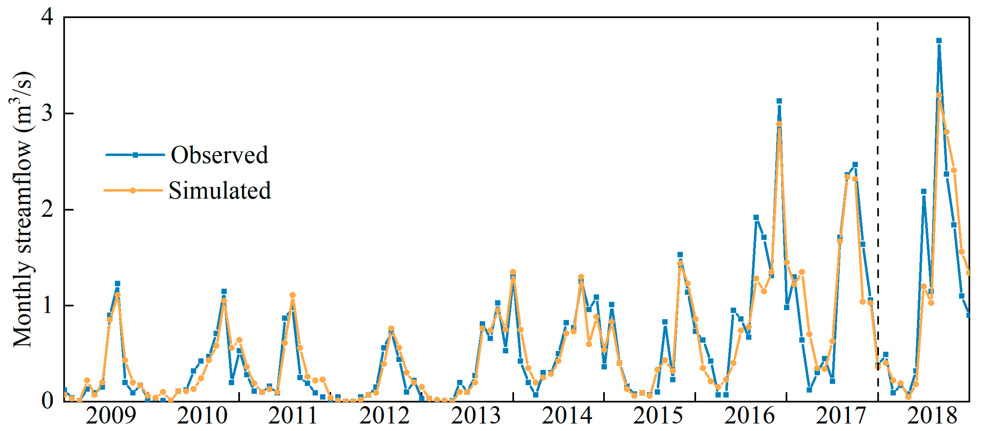
Since most hydrologic gauge stations in YLB were constructed after 2020, only monthly streamflow data from CR are available for the period of 2009–2018. Streamflow data for 2009–2017 was used to calibrate SWAT model parameters, while 2018 data validated model performance. Calibration and validation were conducted using the LU2010 land use dataset. Sensitive parameters in the SWAT model were identified via sensitivity analysis and calibrated using the SUFI-2 (Sequential Uncertainty Fitting Procedure Version 2) algorithm in SWAT-CUP. Model performance was evaluated using the widely used indexes as correlation coefficient (R2) and Nash–Sutcliffe efficiency coefficient (NSE). The formulas for R2 and NSE calculation are outlined as follows:
R 2 = i = 1 n ( o b s i o b s ¯ ) ( s i m i s i m ¯ ) 2 i = 1 n ( o b s i o b s ¯ ) 2 i = 1 n ( s i m i s i m ¯ ) 2
N S E = 1 i = 1 n ( s i m i o b s i ) 2 i = 1 n ( o b s i o b s ¯ ) 2
where obsi and simi are the observed and simulated streamflows at the ith time step, respectively; and o b s ¯ and s i m ¯ are the observed and simulated averaged streamflows, respectively.

3. Results

3.1. Model Performance

Hydrological sensitive parameters in the SWAT model governing watershed processes primarily include variables controlling the surface runoff, soil moisture dynamics, groundwater recharge, evapotranspiration partitioning, lateral subsurface flow, time of concentration, and channel routing mechanisms [51,52]. Table 4 lists the parameters’ settings used in the calibration and sensitivity analysis of this study. Through the sensitivity analysis, we identified the most sensitive parameters affecting streamflow as CN2 (p-value = 0.002), ALPHA_BF (p-value = 0.008), CN_N2 (p-value = 0.027), GW_DELAY (p-value = 0.070), and SOL_AWC (p-value = 0.070). After the model calibration, the model achieved an R2 value of 0.88 and an NSE value of 0.89 during the calibration period (2009–2017) and an R2 value of 0.83 and an NSE value of 0.84 during the validation period (2018), as shown in Figure 5. Collectively, the results from the calibration and validation demonstrate that the SWAT model adequately represented streamflow dynamics in the YLB.
The optimized model parameters were subsequently applied to other subbasins, considering their similar patterns in critical physical–chemical characteristics, such as the land use, DEM, slope and soil conditions, affecting the streamflow.

3.2. Hydrological Responses to Land Use Change

3.2.1. Landscape Patterns and Changes

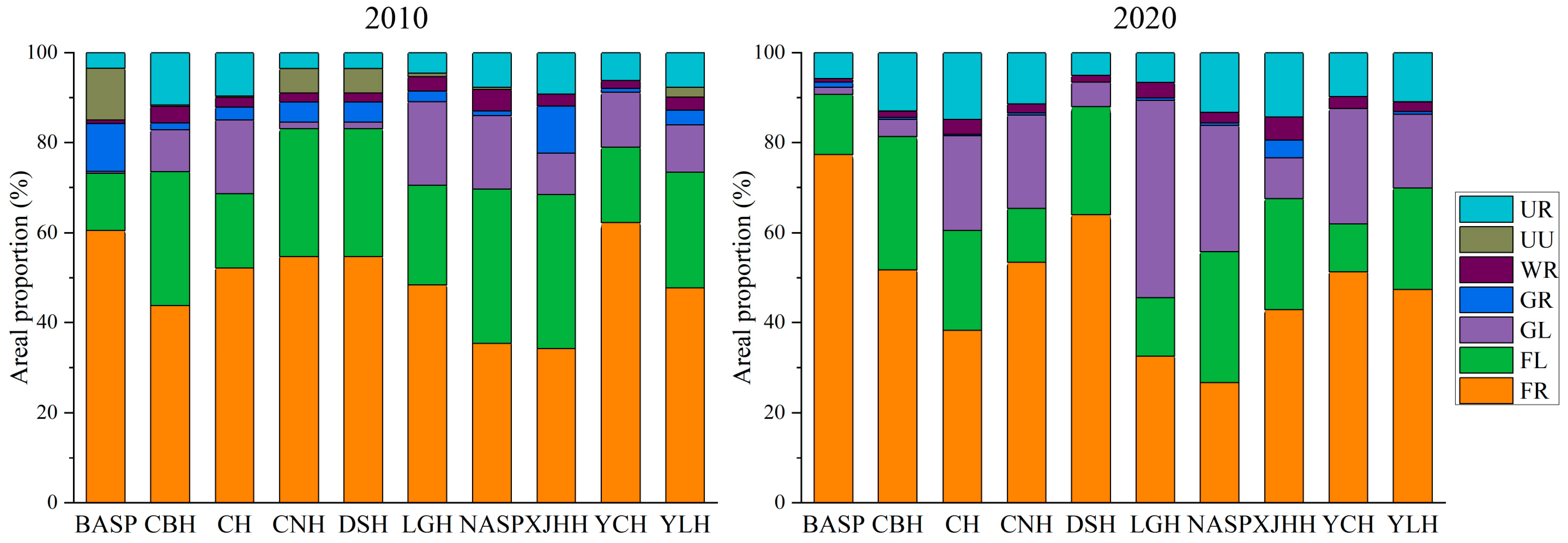
The land use in the YLB presents significant spatial differences (shown in Figure 4e,f). Also, the areal proportion of different land use types in the YLB and subbasins changed significantly from 2010 to 2020. In 2010, FR was the major land use type of the basin (48%), followed by FL (26%), then GL (11%), UR (8%), GR (3%), WR (3%), and UU (3%). However, in 2020, the area proportions of FR, FL, GL, UR, GR, WR, and UU at the whole scale changed to 47%, 22%, 16%, 11%, 1%, 2%, and less than 0.1%. From 2010 to 2020, the basin exhibited an apparent land surface modification, including a loss of area in the land use types of FL (−19.3 km2), GR (−11.71 km2), UU (−7.26 km2), and FR (−1.14 km2), while other land use types expanded, such as GL (+28.25 km2), UR (+10.06 km2), and WR (+1.11 km2). The land use patterns of 2010 and 2020 at the subbasin scale are presented in Figure 6. As shown in Figure 6, FR was the dominant land use type in all subbasins in 2010, accounting for 34–62% of subbasin areas, followed by FL, which accounted for 13–35%. In 2020, the proportion of FR ranged from 27% to 77% and FL from 11% to 30%. In addition, the proportions of GL and UR showed a significant increase in most subbasins from 2010 to 2020.
Figure 7 presents the land use transitions in the YLB and its subbasins from 2010 to 2020. As shown in Figure 7a, the LUCC at the whole watershed scale was mainly dominated by the conversion of FR to GL (24.40 km2), FR to FL (11.44 km2), FL to FR (16.59 km2), FL to UR (11.53 km2), and FL to GL (11.87 km2). At the subbasin scale, land use transitions presented a significant spatial heterogeneity across the subbasins. Specifically, the LUCC in BASP was dominated by FR, and, as shown in Figure 7b, the land use modification was characterized by the conversion from UU and GR (2.85 km2) to FR (2.20 km2), as well as the exchange between FR and FL (0.99 km2 of FR converting to FL and 1.14 km2 of FL converting to FR), which resulted in a 16.6% areal increase in FR, alongside decreases of 9.8% in GR and 11.4% in UU.
CBH is the largest subbasin in the YLB, where FR and FL accounted for 43.8% and 27.9% of the subbasin area in 2010. The major LUCC in CBH included the conversion of FL to UR (2.03 km2) and FR (3.56 km2), FR to FL (1.66 km2), UU to FR (2.20 km2), and GR to FR (143 km2), as shown in Figure 7c, resulting in an 8.0% areal increase in FR and a 5.5% decrease in GL.
For CH (shown in Figure 7d), the land use types conversion of FR to GL (7.76 km2); FL (2.31 km3) and UR (1.46 km2); and FL to GL (4.42 km2), UR (4.06 km2), and FR (3.37 km2) dominated the land use change in the subbasin, resulting in FR decreasing by 13.6% while FL, UR, and GL increased by 5.8%, 5.2%, and 4.4%, respectively.
For CNH (shown in Figure 7e), the land use change mainly included FL converting to FR (1.57 km2), UR (0.97 km2), and GL (0.85 km2), FR converting to GL (1.74 km2) and FL (0.98 km2), as well as GL converting to FR (0.94 km2), resulting in a decrease in FL by 16.4% as well as an increase in GL by 19.2%.
The land use alternation in LGH (Figure 7f) was dominated by the conversion of FR to GL (7.18 km2) and FL to GL (2.97 km2) and FR (1.44 km2), resulting in an 25.3% increase in GL but decreases of 9.1% in FL and 15.7% in FR, respectively.
In subbasin DSH, the land use change (Figure 7g) mainly included the conversion of FL to FR (1.62 km2) and GL (0.55 km2) and FR to FL (1.07 km2), leading to an 8.8% increase in FR and a 4.4% increase in GL.
NASP featured an 11.5% increase in GL, with FR and FL decreasing by 8.7% and 5.1%, respectively, which was mainly attributed to the conversion of FR to GL (4.38 km2) and FL to GL (1.47 km2) and UR (1.83 km2), as shown in Figure 7h.
The subbasin of XJHH is the smallest subbasin in the YLB with a total area of 7.61 km2. The primary land use conversion that occurred in XJHH (shown in Figure 7i) was dominated by the conversion of FL to UR (0.45 km2) and FR (0.41 km2), as well as GR to FR (0.52 km2), leading to a 9.5% increase in FR and a 4.8% increase in UR, while FL and GR decreased by 9.0% and 7.1%, respectively.
In YCH, land use transition (shown in Figure 7j) was dominated by the conversion of FR to GL (1.42 km2) and FL to GR (0.36 km2), UR (0.39 km2), and FR (0.41 km2), collectively resulting in a 13.2% increase in GL, while FR and FL areas decreased by 11.1% and 6.3%, respectively.
The LUCC dynamics in the YLB were primarily driven by urban expansion and ecosystem protection measures implemented over the past decade. Over the past decades, the land demand for urban areas and economic garden land in the basin has been driven by the population growth and the rapid development of the Shiping regional economy. On the other hand, the YLB has faced persistent water resource risks and nutrient pollution challenges in recent decades [53]. To address these issues, local authorities have conducted various environmental protection and ecological restoration measures in recent years. Since 2010, numerous environmental protection projects have been implemented to enhance the basin’s ecological health, such as the restoration of degraded ponds and marshes into wetland and large-scale reforestation on mountains to prevent erosion. Additionally, strict regulations have been introduced to manage large-scale livestock and poultry farming along the lake and rivers, aiming to control the nutrient loading from agricultural activities into the lake. Consequently, the observed land use changes were predominantly influenced by the expansion of urban and economic garden land, alongside ecological protection measures [39].

3.2.2. Streamflow Changes Response to Land Use Alternations

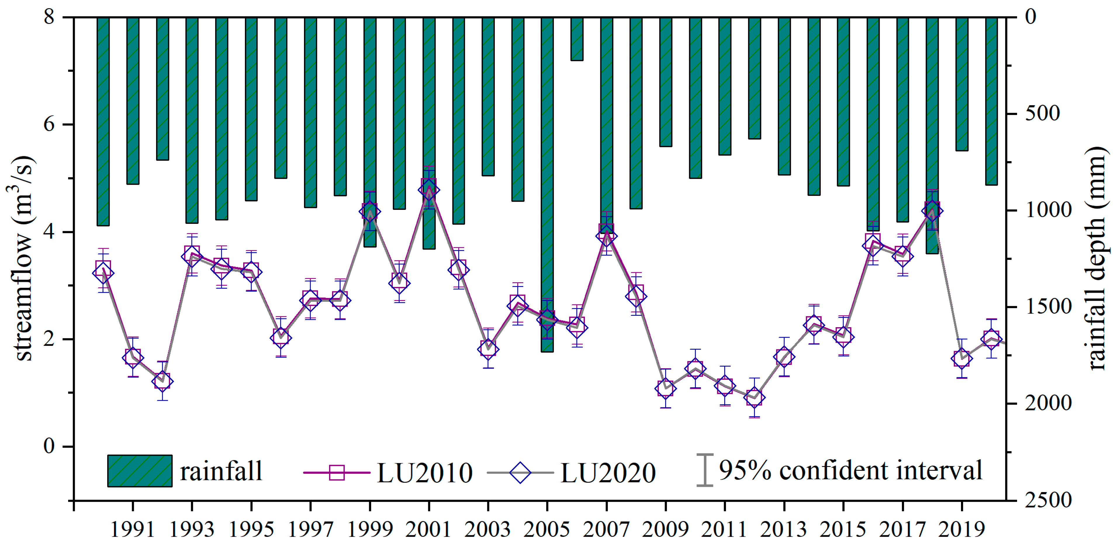
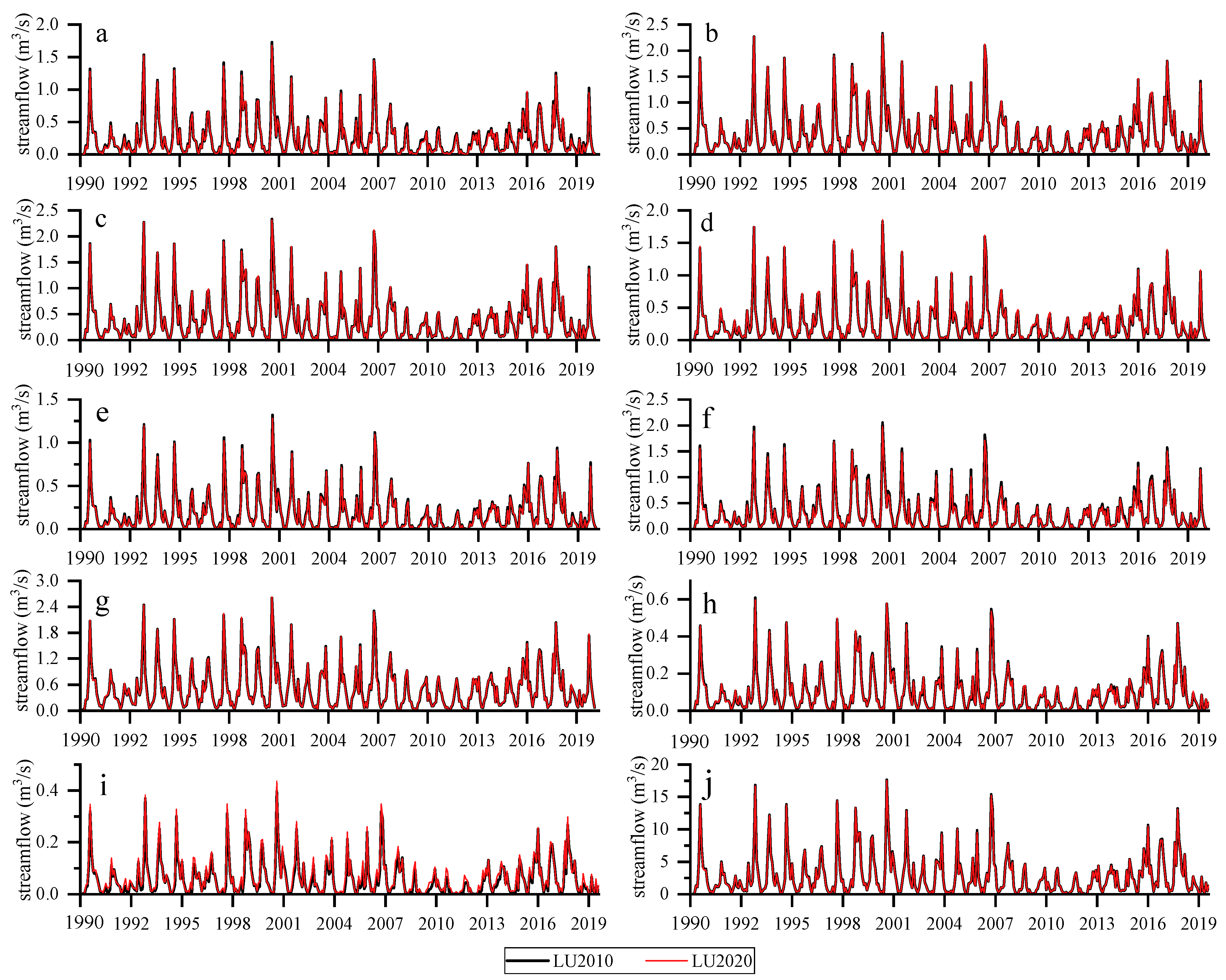
To address the impact of the LUCC on the watershed hydrology, we evaluated the streamflow of the basin over a long historical period from 1990 to 2020 under two land use scenarios of LU2010 and LU2020, representing the land use pattern in 2010 and 2020, respectively. The time series of the annual streamflow from 1990 to 2020 under distinct land use patterns is presented in Figure 8. Generally, the annual streamflow shows a good consistency with the annual rainfall. Under the land use condition of LU2010, the land of the YLB yields an annual streamflow of 2.57 ± 1.08 m3/s (mean ± SD), varying in the range of 0.9–4.85 m3/s, while under LU2020 the annual streamflow of the YLB is 2.53 ± 1.05 m3/s (mean ± SD), varying in the range of 0.91–4.77 m3/s. Although the mean value of the streamflow shows a marginal declining trend (1.21%) under LU2020 compared to LU2010, there is no significant statistic difference (p = 0.90 with paired t-test) between the two land use conditions, indicating that the LUCC that occurred between 2010 and 2020 did not cause a significant alternation in hydrological processes linked to the streamflow at the whole watershed scale. Compared to the annual streamflow, the monthly streamflow in the YLB (shown in Figure 7j) shows a more significant fluctuation, ranging between 0.027 and 17.66 m3/s under LU2010 and ranging between 0.028 and 17.54 m3/s under LU2020, respectively. Similarly to the annual streamflow, the monthly streamflow also presented no significant difference (p = 0.88 with paired t-test) between the two land use conditions.
The subbasins represent a noticeable spatial difference in the streamflows. The annual streamflow in BASP, CH, DSH, LGH, NASP, CBH, CNH, XJHH, and YCH was 0.23 ± 0.09 m3/s, 0.69± 0.33 m3/s, 0.17 ± 0.07 m3/s, 0.29 ± 0.13 m3/s, 0.47 ± 0.14 m3/s, 0.35 ± 0.14 m3/s, 0.24 ± 0.11 m3/s, 0.0055 ± 0.0025 m3/s, and 0.09 ± 0.04 m3/s under the LU2010 land use condition and 0.22 ± 0.10 m3/s, 0.68 ± 0.31 m3/s, 0.16 ± 0.07 m3/s, 0.27 ± 0.12 m3/s, 0.47 ± 0.14 m3/s, 0.35 ± 0.14 m3/s, 0.25 ± 0.11 m3/s, 0.0063 ± 0.0024 m3/s, and 0.08 ± 0.04 m3/s (mean ± SD) under the LU2020 land use condition, respectively. Although the change in the land use from 2010 to 2020 resulted in the exhibition of an increasing trend of annual streamflows by 3.4%, 0.5%, 3.8%, 5.9%, 0.5%, 0.7%, and 14.2% in BASP, CH, DSH, LGH, NASP, YCH, and XJHH, respectively, while there was a decreasing trend of annual streamflows by 0.3% and 2.3% in CBH and CNH, respectively, there is no statistically significant difference in the annual streamflow with p-values ranging from 0.20 to 0.94 across the subbasins. Figure 9 shows the monthly streamflow time series of the subbasins. The monthly streamflow in BASP, CH, DSH, LGH, NASP, CBH, CNH, XJHH, and YCH had a range of 0–1.73 m3/s, 0–5.16 m3/s, 0–1.32 m3/s, 0–2.05 m3/s, 0.02–2.60 m3/s, 0–2.33 m3/s, 0–1.83 m3/s, 0–0.39 m3/s, and 0–0.60 m3/s, respectively, under LU2010 and 0–1.68 m3/s, 0–5.17 m3/s, 0–1.28 m3/s, 0–1.98 m3/s, 0.02–2.63 m3/s, 0–2.32 m3/s, 0–1.85 m3/s, 0–0.43 m3/s, and 0–0.59 m3/s, respectively, under LU2020. Similarly to the annual streamflow, there is no statistically significant difference in the monthly streamflow with p-values ranging from 0.08 to 0.96 across the subbasins.
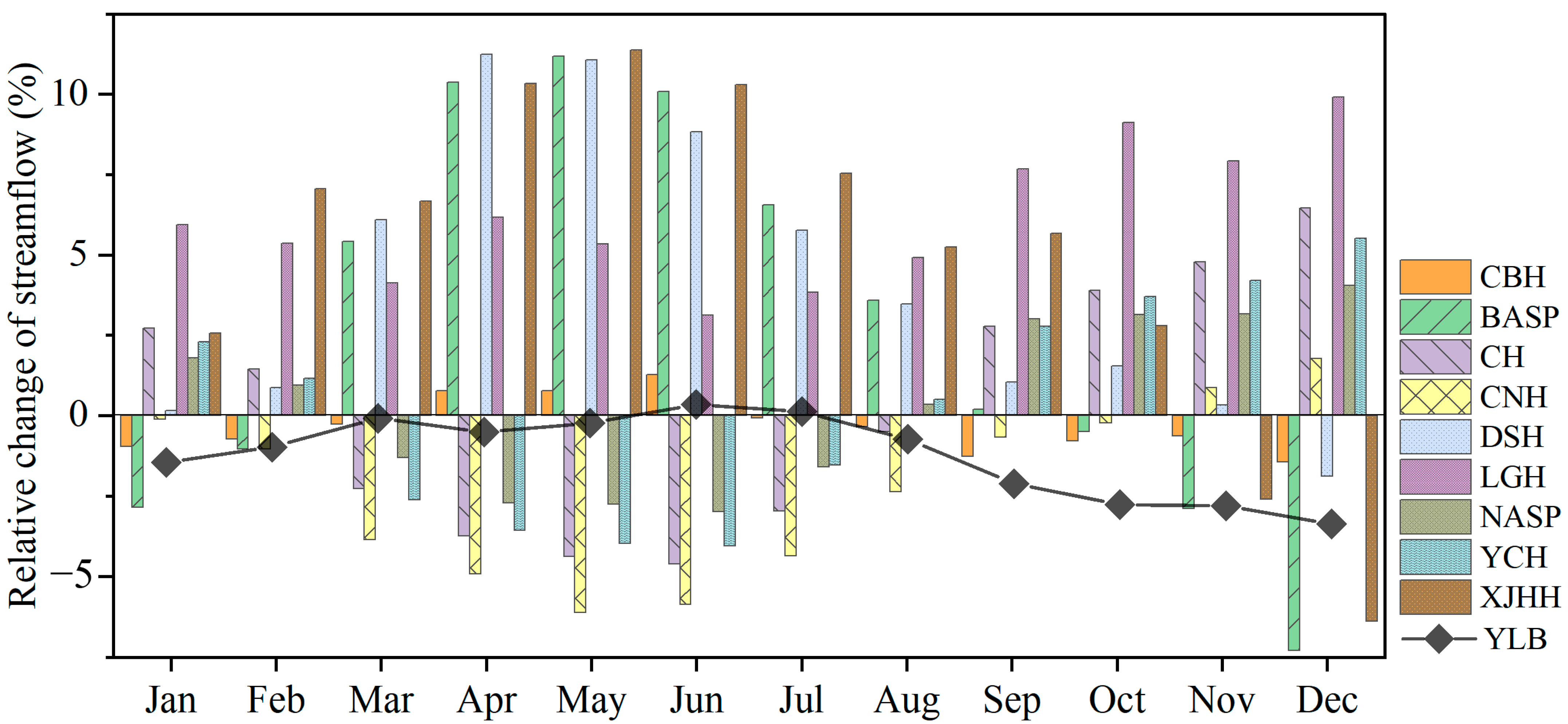
With the normalized analysis, the inter-monthly pattern of relative changes in the streamflow response to shifts in land use types between 2010 and 2020 is shown in Figure 10. The analysis results indicate that the streamflow change exhibits significant inter-monthly variations across the subbasins. Specifically, the streamflow in BASP, DSH, and XJHH becomes more concentrated between March and August, with the monthly streamflow increasing up to 11%, whereas NASP, YCH, CH, and CNH demonstrate an increased streamflow in dry seasons but a decline in wet seasons. LGH experiences a significant enhancement in the streamflow across all months, primarily driven by the extensive land use transfer from FR to GL. In contrast, CBH presents a stable streamflow in both scenarios, with the change in the streamflow across all months being less than 1%. The variation in relative changes in the streamflow across the subbasins is mainly attributed to the differences in land use transitions.

3.3. Projection of Future Streamflow Under Climate Change

3.3.1. Projected Future Temperature

Table 5 summarizes the statistical characteristics, i.e., the mean value, trend index, standard deviation, and coefficient of variation, of the projected temperatures of GCMs from NEX-GDDP-CMIP6. The data suggest a significant upward trend of temperature in the future (R2 ranging from 0.67 to 0.81, p-value < 0.05) according to four GCMs, i.e., ACCESS-CM2, ACCESS-ESM1.5, BCC-CSM2-MR, and NorESM2-LM. Among the SSP scenarios, SSP585 exhibits the highest values of annual mean temperature, followed by SSP370 and SSP245. However, SSP370 demonstrates the highest overall warming trend across all GCMs, with the rate of change in the temperature ranging from +0.034 °C/year to +0.060 °C/year, compared to from +0.025 °C/year to +0.043 °C/year under SSP245 and from +0.022 °C/year to +0.045 °C/year under SSP585. A similar trend for the annual daily maximum temperature is observed as well, albeit it is associated with less confidence, which is primarily due to the more frequent extreme heat events—previous studies projected the frequency of heatwave occurrences in the future will be greatly increased, which is attributed to CC [54]. The projected future temperature in the study area illustrates a potential intensification of the regional warming in the study period. Since the region has been facing a prolonged water scarcity in recent decades due to strong evaporation and deficient rainfall [55], the persistent rise in temperature is expected to intensify the evaporation process in the future, further exacerbating the water resource crisis in the basin.

3.3.2. Projected Future Precipitation

Table 6 summarizes the statistical characteristics, i.e., the mean value, trend index, standard deviation, and coefficient of variation, of projected precipitations of four GCMs from NEX-GDDP-CMIP6. The annual rainfall depth from the GCMs aligns well with historical observations at the Shiping meteorological station during the reference period in the YLB, except the period of 2009–2013 when a prolonged drought occurred in Southwest China. The projection overestimates the rainfall by 53% during that period. Although there are considerable uncertainties in future climate projections [56,57], all GCMs in this study project a relatively consistent mean annual rainfall, with a range from 1030 to 1098 mm between 2015 and 2060. The ensemble of the four GCMs predicts that the mean annual rainfall will be 1077 mm/year under the SSP245 scenario, 1052 mm/year under the SSP370 scenario, and 1075 mm/year under the SSP585 scenario. In addition, there is no coincident rainfall tendency over the projected period observed across the SSP scenarios. Specifically, under the SSP245 scenario, all GCMs indicate a general increasing trend in the annual rainfall from 2015 to 2060, with annual variations ranging from +0.01 mm/year to +1.91 mm/year. Under the SSP370 scenario, ACCESS-CM2 and NorESM2-LM project a decreasing trend in the annual rainfall, with a decreasing rate of −1.09 mm/year and −0.56 mm/year, respectively, while ACCESS-ESM1.5 and BCC-CSM2-MR show an increasing trend in the annual rainfall, with an increasing rate of +0.01 mm/year and +0.58 mm/year, respectively. Under the SSP585 scenario, all GCMs consistently project decreasing trends in rainfall, with the changing magnitudes ranging from −1.54 mm/year to −0.38 mm/year. The results indicate that the future precipitation trends present strong uncertainties under the current situation.
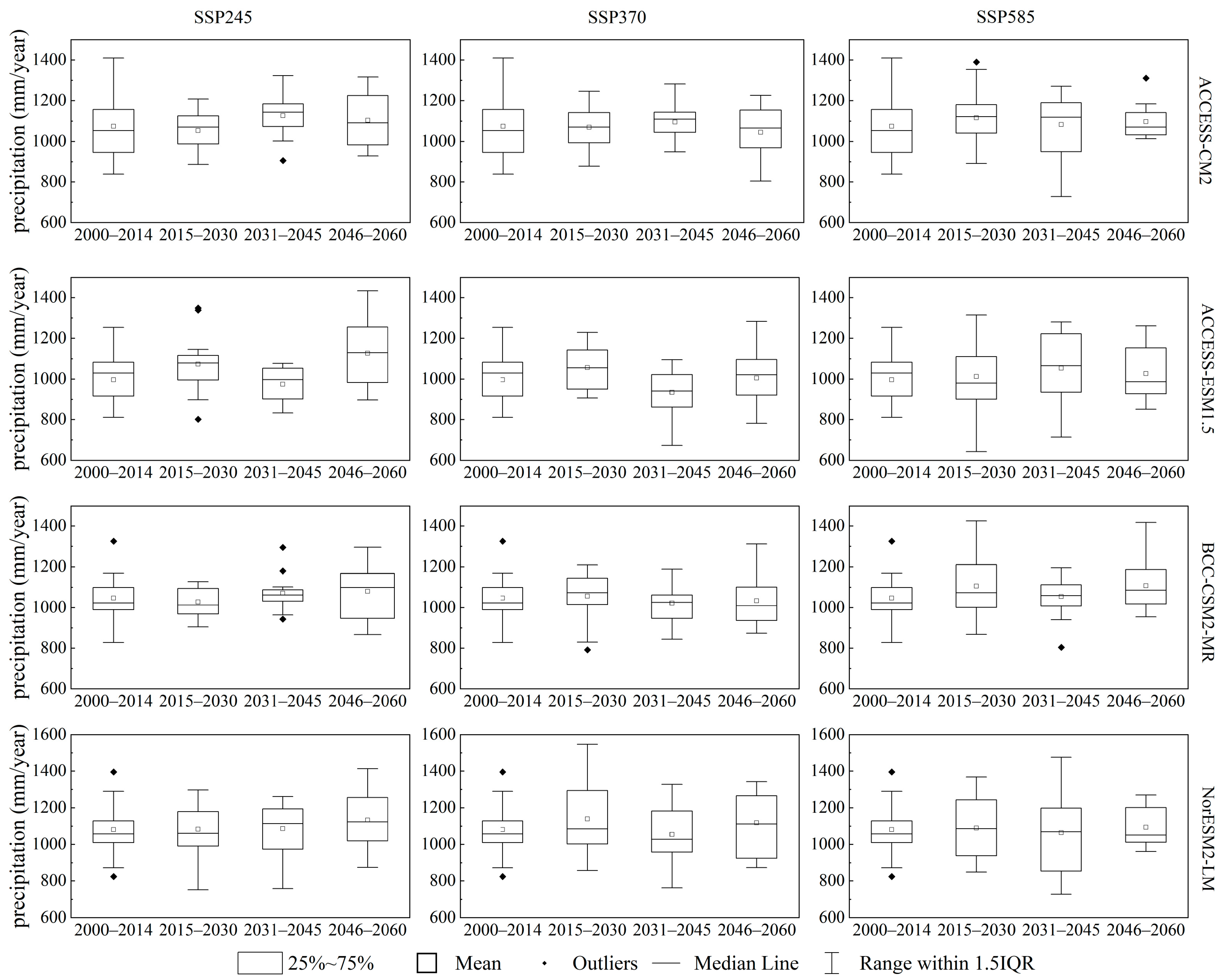
The temporal variation in the projected rainfall across the base period (2000–2014), near-future (2015–2030), mid-future (2031–2045), and far-future (2046–2060) is illustrated in Figure 11. Boxplots of rainfall reveal considerable temporal uncertainties in rainfall distributions, with fluctuations throughout the study period. The projected rainfall from four GCMs does not follow a consistent trend over the entire period. Specifically, the median annual precipitation from the ACCESS-CM2 model shows an increasing trend from the base period to the mid-future, then decreases in the far-future across all SSP scenarios. The median of the annual precipitation under SSP245 and SSP370 from ACCESS-ESM1.5 exhibits an increasing–decreasing–increasing trend, while the median under SSP585 presents an inverse trend in the study period.
The median of the annual precipitation from BCC-CSM2-MR under SSP245 shows a slight decrease by 2030, then increases over 2031–2045 and 2046–2060. Under SSP370 and SSP585, the median of the annual precipitation increases in the near-future, then decreases in the mid-future. The median of the annual precipitation from NorESM2-LM under SSP245 shows an increasing tendency from the near- to mid-future, while under SSP370 the trend is reversed, and under SSP585 there is no significant tendency. As the primary climatic driver of streamflow in watersheds [58], the uncertainty and temporal fluctuation of rainfall will translate into dynamics of water processes in the YLB.

3.3.3. Projected Future Streamflow Dynamics

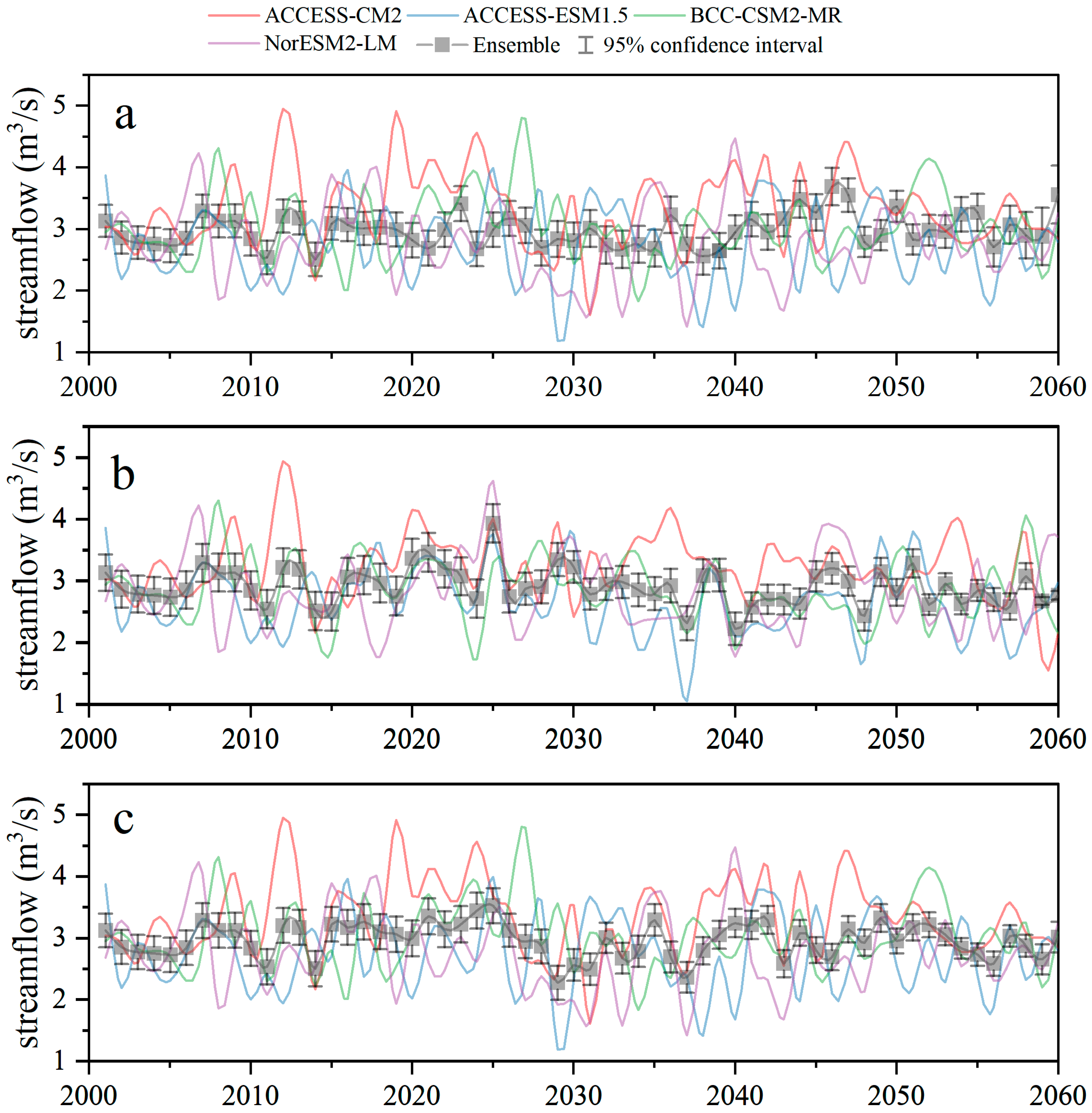
As illustrated in Figure 12, the annual streamflows from 2001 to 2060 present complex variations and large uncertainties. Specifically, during the base period of 2001–2014, the overall annual streamflows were estimated as ranging from 2.60 to 3.38 m3/s, with a mean value of 2.93 ± 0.58 m3/s. The temporal variation in streamflows was consistent with the observations for most of the period, except the extreme drought period (2009–2013) when a prolonged precipitation deficit event occurred in the Southwest of China. Annual streamflows from 2015 to 2060 were projected to range from 2.56 to 3.69 m3/s, with a mean value of 3.00 ± 0.27 m3/s under SSP245 scenarios, from 2.22 to 3.93 m3/s (mean value of 2.90 ± 0.32 m3/s) under SSP370 scenarios, and from 2.28 to 3.53 m3/s (mean value of 2.98 ± 0.29 m3/s) under SSP585 scenarios, respectively. Compared to the reference period, annual streamflows in the future present differences varying from −3.92% to +6.86% under different combinations of GCMs and SSP scenarios.
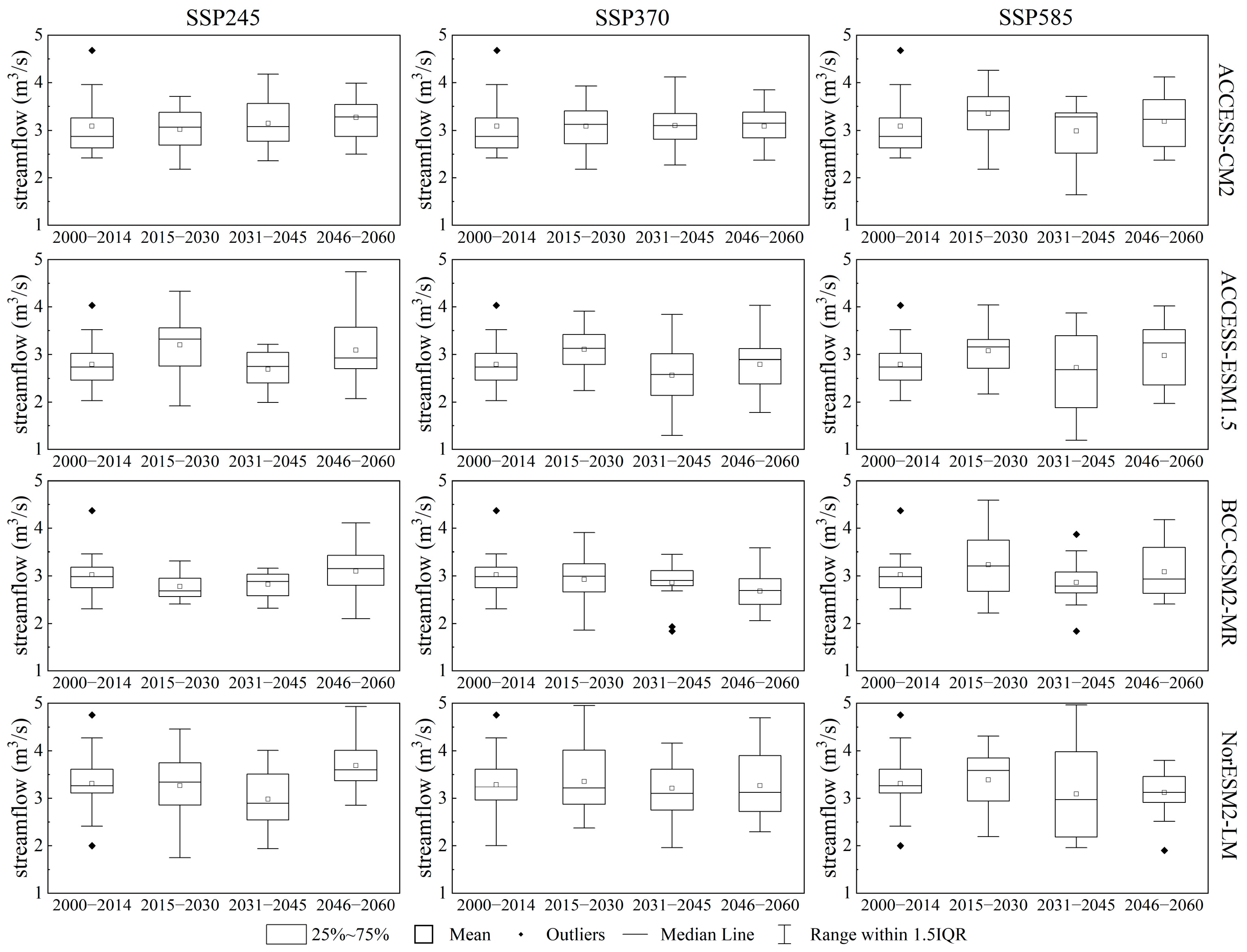
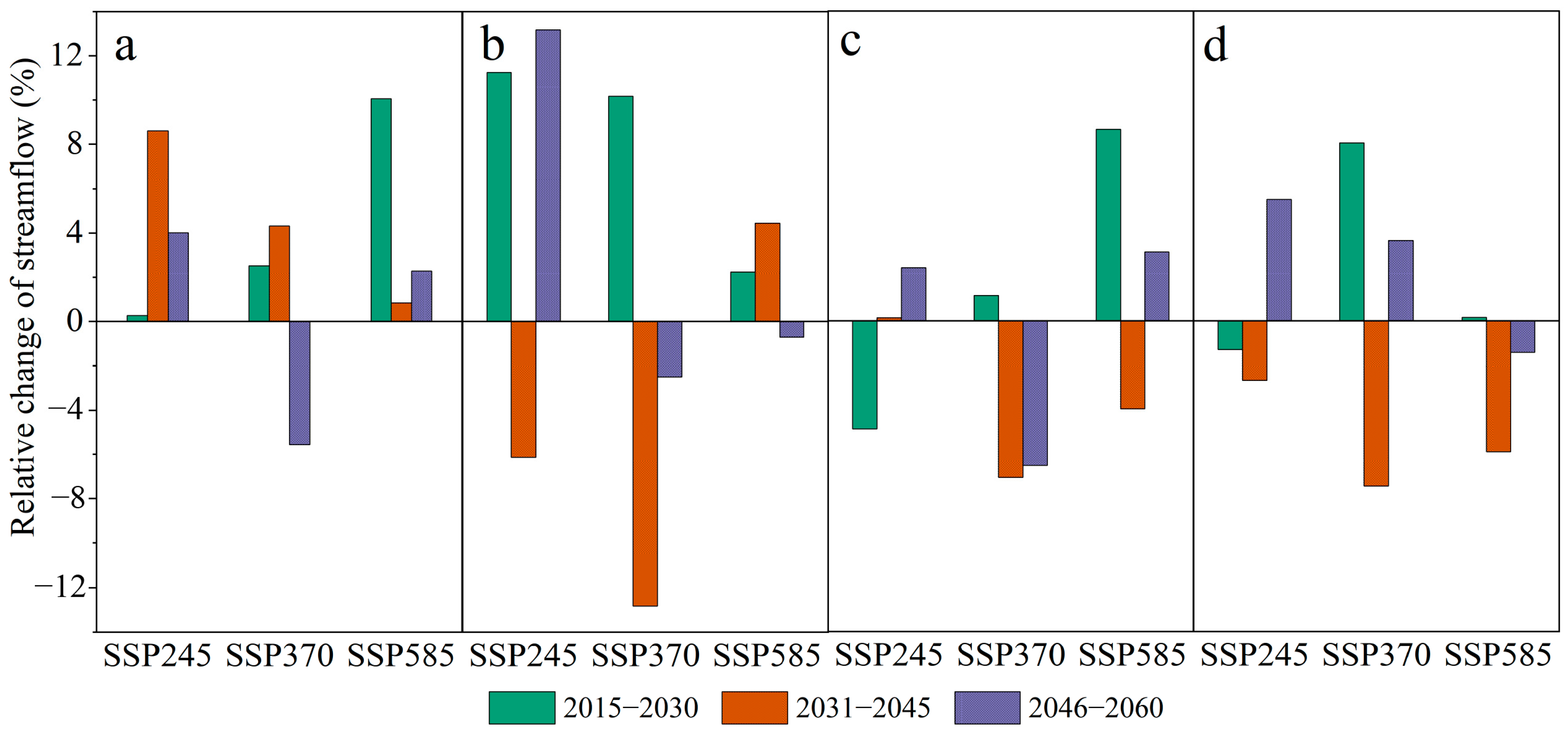
Temporal variability and substantial uncertainty characterize projected streamflow changes over the projection period (2015–2060) under different climate scenarios, as shown in Figure 13. Specifically, under the SSP245 scenario, the ensemble mean annual streamflow exhibits an initial slight decline followed by an upward trend over the projection period, with values of 2.96 m3/s in the near-future, 2.94 m3/s in the mid-future, and 3.11 m3/s in the far-future. For SSP370, the ensemble projected streamflow demonstrates an increase in the near-future (3.07 m3/s), followed by decreases in the mid-future (2.78 m3/s) and far-future (2.84 m3/s). Similarly, the SSP585 scenario simulations show a comparable pattern, with projected values of 3.09 m3/s in the near-future, 2.90 m3/s in the mid-future, and 2.95 m3/s in the far-future. The change in the streamflow indicates that CC exerts a substantial influence on hydrological processes in the YLB, which is characterized by pronounced temporal variability and scenario-dependent uncertainties under different SSPs. The relative change in the streamflow relative to the reference period for GCMs under different SSP scenarios is shown in Figure 14.
The Mann–Kendall test is a non-parametric statistical method broadly used to detect monotonic trends in time series data [59]. To test for potential monotonic trends in the projected streamflow over time driven by GCMs and SSP conditions, a Mann–Kendall test was conducted in this study. As shown in Table 7, most streamflow projections do not show significant monotonic trends, except for specific scenarios. In detail, ACCESS-CM2 under SSP245 resulted in an increasing trend (Zc = 1.97) of the projected streamflow over 2001–2060, while BCC-CMS2-MR under SSP370 resulted in a decreasing trend (Zc = −1.82). In the period of 2015–2030, the streamflow exhibited an increasing trend driven by ACCESS-CM2 under SSP370 (Zc = 1.67) as well as by BCC-CSM2-MR under SSP585 (Zc = 3.11), while NorESM2-LM under SSP585 (Zc = −1.67) resulted in a decreasing trend of streamflow. In 2031–2045, NorESM2-LM and the ensemble under SSP370 (Zc = −1.98) resulted in a decreasing trend of streamflow, while ACCESS-CM2 (Zc = 1.93) and the ensemble (Zc = 1.98) under SSP585 resulted in an increasing trend of streamflow. In 2046–2060, ACCESS-ESM1.5 under SSP245 (Zc = 1.98) and NorESM2-LM under SSP585 (Zc = 1.73) resulted in an increasing trend of streamflow, while BCC-CSM2-MR under SSP245 (Zc = −1.98) resulted in a tendency for the streamflow to decrease.
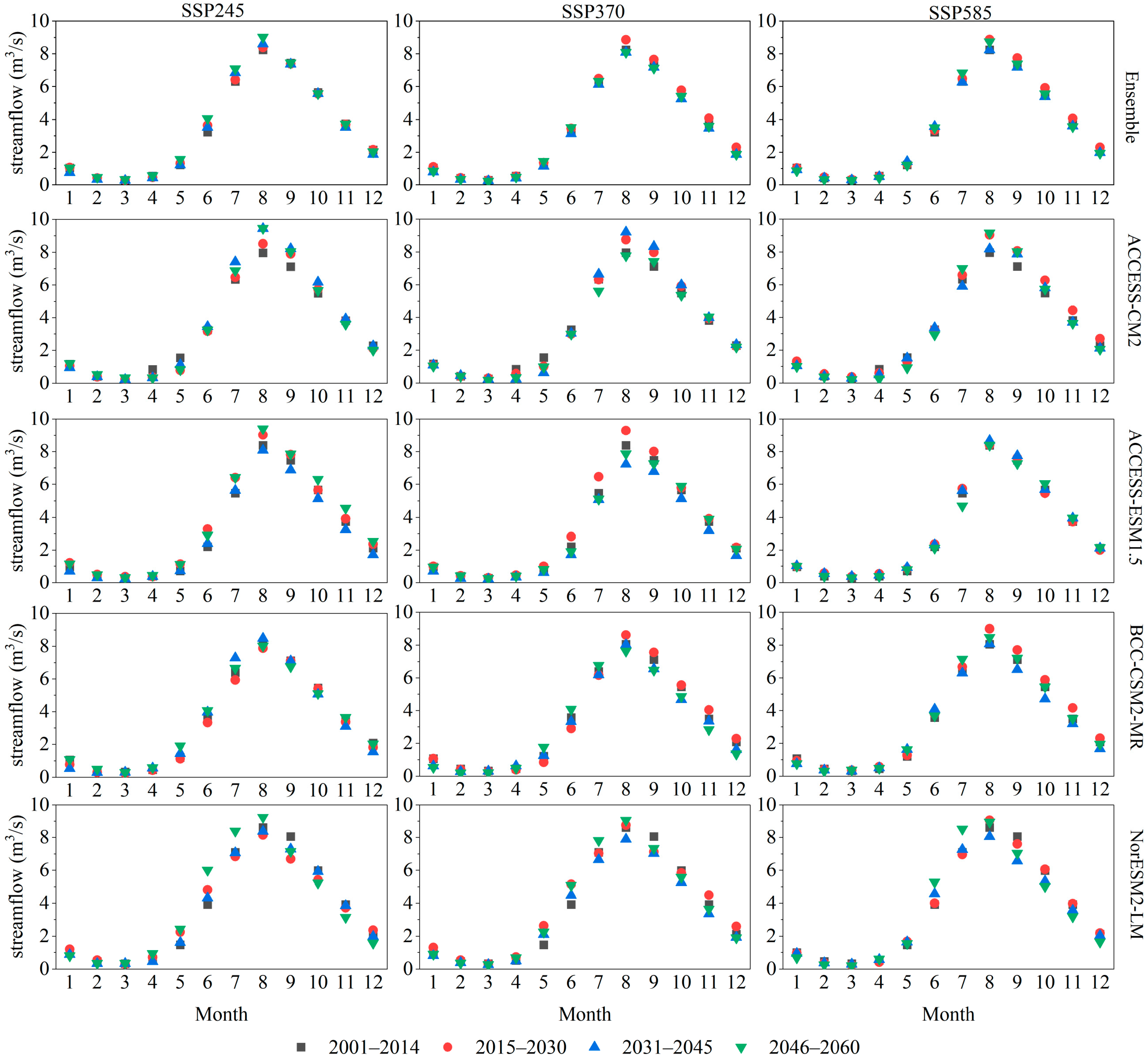
Besides the impact on the annual streamflow volume, CC also exerts a potential influence on the inter-monthly distribution pattern of projected streamflows. As highlighted in Figure 15, hydrological projections across all climate scenarios indicate a consistent enhancement of the streamflow in wet seasons and a decline in dry seasons, with a peak discharge observed in August and a minimum streamflow in March. Specifically, the modeling under the SSP245 scenario typically exhibits a monotonic increase in the wet-season streamflow, with mean values ranging from 5.29 to 5.84 m3/s over the projection period. In contrast, SSP370 and SSP585 scenarios demonstrate increase–decrease–increase trends relative to the baseline period, fluctuating within 5.14–5.57 m3/s and 5.29–5.55 m3/s, respectively. The ensemble mean dry-season streamflow remains relatively stable across all scenarios, varying between 1.78 and 2.10 m3/s.
Additionally, substantial inter-model discrepancies emerge in monthly streamflow distributions. For instance, the ACCESS-CM2 model projects a significant springtime decline (−46% to −12%) and July–October increases (+5% to +18%) across all SSPs. Conversely, ACCESS-ESM1.5 shows pronounced wet-season streamflow enhancements under SSP245 (+8% to +15%) and SSP370 (+6% to +10%), characterized by increase–decrease–increase dynamics, whereas SSP585 yields no significant streamflow changes. The BCC-CSM2-MR model aligns closely with ensemble averages but projects an August–December streamflow intensification (+7% to +18%).
Notably, compared to other GCMs, NorESM2-LM uniquely projects marked July–August increases (+22% to +28%) across all scenarios for the far-future, representing the most divergent behavior among evaluated models.

4. Discussion

4.1. Impacts of Land Use Change on Streamflow

Over the past decades, intensive human activities in the YLB, such as urbanization, the dramatic expansion of economic garden lands, and ecological restoration programs, have greatly modified the landscape pattern of the YLB [40]. From 2010 to 2020, areas of FL, GR, UU, and FR declined by 19.3 km2, 11.71 km2, 7.26 km2, and 1.14 km2, while GL, UR, and WR expanded by 28.25 km2, 10.06 km2, and 1.11 km2, respectively. LUCC usually represents a critical anthropogenic driver that can profoundly alter the hydrologic processes of watersheds [60]. To reveal the potential impact of the land use alternation on the basins’ hydrology, a long-term watershed hydrologic simulation was conducted with the SWAT model under the land use patterns of 2010 and 2020, respectively.
The simulation results illustrated that although there were significant land use transitions in the YLB, the LUCC at the basin scale only caused a marginal decrease in the annual streamflow by 1.21% (p = 0.90). However, previous studies reported much more significant streamflow changes responding to LUCC. For instance, Wu et al. [19] estimated that land cover changes contribute to around 22.8% to 27.5% of the streamflow change in the Upper Fen River Basin, China. Lu et al. [16] reported that the contribution of the LUCC to the runoff depth in the Songnen Plain, China, was from 17.7% to 29.2%. Li et al. [61] suggested that the LUCC in the Jihe watershed contributes up to 90.2% of the streamflow decline. Such differences between our study and references may be caused by the unique tectonic geomorphology in the YLB. Since the YLB is characterized by a fragile karst landscape, the infiltration and water storage capacity of natural land surfaces, e.g., forest and grassland, is strongly restricted, especially on elevated steep slope areas.
Spatial differences in the LUCC at the subbasin scale result in heterogeneous responses in streamflow fluctuations. For example, CH gained 1.88 km2 of farmland and 1.68 km2 of urban area while losing 4.40 km2 of forests. The conversion of natural landscapes to an anthropogenic land use can lead to an increased surface runoff resulting from the reduced infiltration [62]. Such LUCC in CH resulted in a 0.5% increase in streamflow. It should be noted that the impact magnitude of the land use change on the streamflow is also influenced by other characteristics of the watershed, such as soil and slope characteristics.
In addition, the more frequent dry-season streamflow reduction in the basin associated with the LUCC from LU2010 to LU2020 highlights the critical role of land cover in regulating the seasonal water availability. Ecological restoration projects, such as wetland rehabilitation and afforestation, likely increased the water uptake by vegetation during the dry season, exacerbating low-flow conditions. This result is consistent with previous studies in semi-arid basins [61,63], where vegetation restoration reduces the baseflow by enhancing evapotranspiration. Conversely, urbanized subbasins, such as CH and CBH, exhibited increased dry-season flows due to the reduced soil water storage from impervious surfaces, illustrating the hydrological trade-offs of urbanization.

4.2. Impacts of Climate Change on Streamflow and Future Hydrological Risks

The observed rising temperatures (+0.02–+0.04 °C/year) and declining precipitation (−4.4 mm/year) from 1990 to 2020 are consistent with regional climate projections in Southwest China, where climate warming has intensified evaporation and exacerbated water stress in these karst ecosystems [64]. All GCMs and SSP scenarios in this study projected rising temperatures in the future (2015–2060), while precipitation predictions show a remarkable uncertainty as they slightly increase (+0.012–+1.192 mm/year) under SSP245 but generally decrease (−1.54–−0.38 mm/year) under SSP585. Future annual streamflows were projected to vary from −3.92% to +6.86% compared to the reference period according to different GCMs and SSP scenarios. In contrast, a stronger decrease in the future streamflow (−7% to −22%) was predicted in the Dianchi Lake Basin [20].
The mid-future streamflow is projected to reduce by up to 5.9% under high-emission scenarios, e.g., SSP585, suggesting escalating water scarcity in the future, particularly for agricultural and domestic water use. The intensification of extreme events further complicates water resource planning, as demonstrated by the ACCESS-CM2’s projection of 11–18% streamflow increases in wet seasons alongside 12–46% spring declines, highlighting the need for adaptive water resource management.
In addition, the stream projection suggests that although the total amount of precipitation will decline, the temporal distribution of future precipitation tends to be more concentrated in the summer season under scenarios like SSP370 and SSP585. This may amplify seasonal water stress, as shorter wet seasons could limit groundwater recharge while longer dry seasons intensify evaporation. Moreover, projected increases in extreme rainfall events, e.g., from +5% to +28% in July–August under NorESM2-LM, pose dual risks of flash floods and droughts in the basin, challenging flood control and water storage infrastructures in karst regions.

4.3. Implications for Watershed Management and Sustainability

In the YLB, population growth and regional economic development have driven the rapid expansion of urban land and economic garden land since the 2000s. On the other hand, the YLB has faced persistent water resource risks and water pollution challenges in recent decades [53]. To address these issues, local authorities have implemented various environmental protection and ecological restoration measures. Engineering projects, such as the restoration of degraded ponds and wetlands into lakes, and large-scale reforestation have been carried out to enhance the basin’s ecological health. Additionally, strict regulations have been introduced to manage the farmland and economic garden land use along the lake and rivers, aiming to reduce the nutrient pollution from agricultural activities into the lake.
The annual water yield volume of the YLB in the period of 1990–2020 was estimated to reach 84.9 million m3, ranging from 28.3 to 153.0 million m3. As a small watershed, the annual water yield volume of the YLB is much smaller compared to other plateau lake watersheds in Yunnan; e.g., the Dianchi Lake basin has an annual water yield volume of 669 million m3 [65] to 923 million m3 [66].
The findings in this study reinforce the need for integrated water governance that combines climate-resilient land use policies with adaptive infrastructure. For instance, implementing Sponge City technologies in urban areas to enhance stormwater retention and promoting agroforestry in rural subbasins could mitigate both flood and drought risks. Forested areas could be prioritized for water yield conservation through restricting land use change, which preserves their hydrological functions. Ecological restoration strategies, such as planting drought-resistant species instead of water-intensive trees, are critical for climate change mitigation. Furthermore, incorporating LUCC-CC interaction effects into water allocation plans, e.g., inter-basin water transfers during droughts, would enhance the resilience of the semi-closed hydrological system.

4.4. Uncertainties and Research Limitations

In this study, the four GCMs introduce model-specific climatic biases that contribute to uncertainties in streamflow projections, such as NorESM2-LM’s outlier projections of extreme wet-season flows. Meanwhile, accurately simulating the hydrologic processes in karst landscapes with the SWAT is challenging [67]. Additionally, uncertainties regarding hydrology processes in the SWAT mainly include the resolution of the collected data, e.g., the soil, the DEM, climate data and observations, the delineation and the threshold set of the minimum watershed area, as well as the calibration process. Furthermore, the lack of long-term streamflow observations at major streams in the YLB limited the accuracy of flow simulations in the basin. The long-term monitoring of hydrological processes is recommended to improve the comprehensive understanding of the complex hydrology in the basin.

5. Conclusions

This study systematically investigates the hydrological responses to LUCC and CC in the YLB, a fragile plateau karst watershed in Southwest China, using the SWAT model. The historical analysis reveals that LUCC, mainly driven by urbanization, economic agricultural activities, and ecological restorations between 2010 and 2020, induced a marginal decline in the annual streamflow at the basin scale but significantly altered the intra-annual discharge pattern. Dry-season flows decreased due to the spatial heterogeneity in land cover transitions, and subbasins exhibited divergent responses, highlighting the spatial differences in LUCC and hydrologic responses.
CC emerged as the dominant driver of hydrological variability, with a declining precipitation trend strongly correlating with streamflow dynamics. Future projections under SSP245, SSP370, and SSP585 scenarios indicate general streamflow declines, particularly under high-emission pathways, e.g., SSP370 and SSP585. Additionally, intensified extreme rainfall events and seasonal water stress pose combined risks of flash floods and droughts, exacerbating water resource management challenges in this semi-enclosed basin.
The findings highlight the urgent need for adaptive strategies to manage water resources in the YLB, including reducing the scale of water-intensive agriculture and implementing integrated water allocation, ecosystem restoration, and climate-resilient land use policies, to mitigate hydrological shifts in fragile plateau ecosystems. By quantifying the combined impacts of LUCC and CC, this study provides a scientific foundation for sustainable water governance in Southwest China, emphasizing the critical role of proactive management in safeguarding water security amid projected warming and land surface transformations. Furthermore, sufficient hydrological monitoring systems should be implemented promptly to collect the necessary data and refine model projections, addressing uncertainties in climate–hydrology interactions and ensuring robust resilience planning for similar karst watersheds.

Author Contributions

Conceptualization, Z.B. and W.H.; methodology, Z.B. and Y.W.; validation, W.H. and N.S.; investigation, Y.W.; writing—original draft preparation, Z.B. and Y.W.; writing—review and editing, Z.B., Y.W., N.S., H.S., and C.F.; funding acquisition, Z.B. and N.S. All authors have read and agreed to the published version of the manuscript.

Funding

This research was funded by the Yilong Lake Protecting and Governance Research Project (grant number: FDZBHH2021039-3), the Zhuhai Science and Technology Plan Project in the Social Development Field (grant number: 2420004000113), and the Urban Management Bureau of Yinchuan City (grant number: D6401-2024061200008-1).

Data Availability Statement

The original contributions presented in this study are included in the article. Further inquiries can be directed to the corresponding author.

Conflicts of Interest

Authors Y.W. and W.H. are employed by the company China Machinery International Engineering Design and Research Institute Co., Ltd, and author C.F. is employed by the company Bejing Planning and Design Consultants Ltd., China Academy of Urban Planning and Design. The remaining authors declare that the research was conducted in the absence of any commercial or financial relationships that could be construed as a potential conflict of interest.

References

  1. Wang, Y.; Zhang, X.; Peng, P. Spatio-Temporal Changes of Land-Use/Land Cover Change and the Effects on Ecosystem Service Values in Derong County, China, from 1992–2018. Sustainability 2021, 13, 827. [Google Scholar] [CrossRef]
  2. Romulo, C.L.; Posner, S.; Cousins, S.; Hoyle Fair, J.; Bennett, D.E.; Huber-Stearns, H.; Richards, R.C.; McDonald, R.I. Global state and potential scope of investments in watershed services for large cities. Nat. Commun. 2018, 9, 4375. [Google Scholar] [CrossRef] [PubMed]
  3. Cao, Z.; Wang, S.; Luo, P.; Xie, D.; Zhu, W. Watershed Ecohydrological Processes in a Changing Environment: Opportunities and Challenges. Water 2022, 14, 1502. [Google Scholar] [CrossRef]
  4. Edwards, P.J.; Williard, K.W.J.; Schoonover, J.E. Fundamentals of Watershed Hydrology. J. Contemp. Water Res. Educ. 2015, 154, 3–20. [Google Scholar] [CrossRef]
  5. Kayitesi, N.M.; Guzha, A.C.; Mariethoz, G. Impacts of land use land cover change and climate change on river hydro-morphology—A review of research studies in tropical regions. J. Hydrol. 2022, 615, 128702. [Google Scholar] [CrossRef]
  6. Vörösmarty, C.J.; McIntyre, P.B.; Gessner, M.O.; Dudgeon, D.; Prusevich, A.; Green, P.; Glidden, S.; Bunn, S.E.; Sullivan, C.A.; Liermann, C.R.; et al. Global threats to human water security and river biodiversity. Nature 2010, 467, 555–561. [Google Scholar] [CrossRef]
  7. Wang, X.; He, K.; Dong, Z. Effects of climate change and human activities on runoff in the Beichuan River Basin in the northeastern Tibetan Plateau, China. Catena 2019, 176, 81–93. [Google Scholar] [CrossRef]
  8. Wang, S.; Cai, T.; Wen, Q.; Yin, C.; Han, J.; Zhang, Z. Spatiotemporal Dynamics of Ecosystem Water Yield Services and Responses to Future Land Use Scenarios in Henan Province, China. Water 2024, 16, 2544. [Google Scholar] [CrossRef]
  9. Zhou, S.; Yu, B.; Lintner, B.R.; Findell, K.L.; Zhang, Y. Projected increase in global runoff dominated by land surface changes. Nat. Clim. Change 2023, 13, 442–449. [Google Scholar] [CrossRef]
  10. Fang, D.; Hao, L.; Cao, Z.; Huang, X.; Qin, M.; Hu, J.; Liu, Y.; Sun, G. Combined effects of urbanization and climate change on watershed evapotranspiration at multiple spatial scales. J. Hydrol. 2020, 587, 124869. [Google Scholar] [CrossRef]
  11. Oudin, L.; Salavati, B.; Furusho-Percot, C.; Ribstein, P.; Saadi, M. Hydrological impacts of urbanization at the catchment scale. J. Hydrol. 2018, 559, 774–786. [Google Scholar] [CrossRef]
  12. Abebe, Y.; Tesfamariam, S. Climate Change Impact and Adaptation for Urban Drainage Systems. In Climate Adaptation Engineering; Bastidas-Arteaga, E., Stewar, M.G., Eds.; Butterworth-Heinemann: Oxford, UK, 2019; pp. 73–98. [Google Scholar]
  13. Yang, M.; Mohammad Yusoff, W.F.; Mohamed, M.F.; Jiao, S.; Dai, Y. Flood economic vulnerability and risk assessment at the urban mesoscale based on land use: A case study in Changsha, China. J. Environ. Manag. 2024, 351, 119798. [Google Scholar] [CrossRef]
  14. Wu, Y.; Yin, X.; Zhou, G.; Bruijnzeel, L.A.; Dai, A.; Wang, F.; Gentine, P.; Zhang, G.; Song, Y.; Zhou, D. Rising rainfall intensity induces spatially divergent hydrological changes within a large river basin. Nat. Commun. 2024, 15, 823. [Google Scholar] [CrossRef]
  15. You, Q.; Cai, Z.; Wu, F.; Jiang, Z.; Pepin, N.; Shen, S.S.P. Temperature dataset of CMIP6 models over China: Evaluation, trend and uncertainty. Clim. Dyn. 2021, 57, 17–35. [Google Scholar] [CrossRef]
  16. Lu, Z.; Zhang, J.; Li, C.; Dong, Z.; Lei, G.; Yu, Z. Effects of land use change on runoff depth in the Songnen Plain, China. Sci. Rep. 2024, 14, 24464. [Google Scholar] [CrossRef]
  17. van der Laan, E.; Nunes, J.P.; Dias, L.F.; Carvalho, S.; Mendonca Dos Santos, F. Assessing the climate change adaptability of sustainable land management practices regarding water availability and quality: A case study in the Sorraia catchment, Portugal. Sci. Total Environ. 2023, 897, 165438. [Google Scholar] [CrossRef]
  18. Tang, J.; Song, P.; Hu, X.; Chen, C.; Wei, B.; Zhao, S. Coupled effects of land use and climate change on water supply in SSP–RCP scenarios: A case study of the Ganjiang River Basin, China. Ecol. Indic. 2023, 154, 110745. [Google Scholar] [CrossRef]
  19. Wu, X.; Zhao, X.; Chen, P.; Zhu, B.; Cai, W.; Wu, W.; Guo, Q.; Iribagiza, M.R. Assessing the effects of combined future climate and land use/cover changes on streamflow in the Upper Fen River Basin, China. J. Hydrol. Reg. Stud. 2024, 53, 101853. [Google Scholar] [CrossRef]
  20. Zhou, J.; He, D.; Xie, Y.; Liu, Y.; Yang, Y.; Sheng, H.; Guo, H.; Zhao, L.; Zou, R. Integrated SWAT model and statistical downscaling for estimating streamflow response to climate change in the Lake Dianchi watershed, China. Stoch. Environ. Res. Risk Assess. 2015, 29, 1193–1210. [Google Scholar] [CrossRef]
  21. Duan, Z.; Wang, M.; Chang, X.; Gao, W. Response of river-lake hydrologic regimes to local climate change in the Yunnan-Guizhou Plateau region, China. Reg. Environ. Change 2020, 20, 122. [Google Scholar] [CrossRef]
  22. Zhang, L.; Karthikeyan, R.; Bai, Z.; Srinivasan, R. Analysis of streamflow responses to climate variability and land use change in the Loess Plateau region of China. Catena 2017, 154, 1–11. [Google Scholar] [CrossRef]
  23. Xiao, F.; Wang, X.; Fu, C. Impacts of land use/land cover and climate change on hydrological cycle in the Xiaoxingkai Lake Basin. J. Hydrol. Reg. Stud. 2023, 47, 101422. [Google Scholar] [CrossRef]
  24. Nodine, T.G.; Conley, G.; Riihimaki, C.A.; Holland, C.; Beck, N.G. Modeling the impact of future rainfall changes on the effectiveness of urban stormwater control measures. Sci. Rep. 2024, 14, 4082. [Google Scholar] [CrossRef] [PubMed]
  25. Bao, J.; Feng, J.; Wang, Y. Dynamical downscaling simulation and future projection of precipitation over China. J. Geophys. Res. Atmos. 2015, 120, 8227–8243. [Google Scholar] [CrossRef]
  26. Feng, D.; Tan, Z.; He, Q. Physics-Informed Neural Networks of the Saint-Venant Equations for Downscaling a Large-Scale River Model. Water Resour. Res. 2023, 59, e2022WR033168. [Google Scholar] [CrossRef]
  27. O’Neill, B.C.; Tebaldi, C.; van Vuuren, D.P.; Eyring, V.; Friedlingstein, P.; Hurtt, G.; Knutti, R.; Kriegler, E.; Lamarque, J.-F.; Lowe, J.; et al. The Scenario Model Intercomparison Project (ScenarioMIP) for CMIP6. Geosci. Model Dev. 2016, 9, 3461–3482. [Google Scholar] [CrossRef]
  28. Gou, J.; Miao, C.; Duan, Q.; Tang, Q.; Di, Z.; Liao, W.; Wu, J.; Zhou, R. Sensitivity Analysis-Based Automatic Parameter Calibration of the VIC Model for Streamflow Simulations Over China. Water Resour. Res. 2020, 56, e2019WR025968. [Google Scholar] [CrossRef]
  29. Amiri, S.N.; Khoshravesh, M.; Valashedi, R.N. Assessing the effect of climate and land use changes on the hydrologic regimes in the upstream of Tajan river basin using SWAT model. Appl. Water Sci. 2023, 13, 130. [Google Scholar] [CrossRef]
  30. Gassman, P.W.; Sadeghi, A.M.; Srinivasan, R. Applications of the SWAT Model Special Section: Overview and Insights. J. Environ. Qual. 2014, 43, 1–8. [Google Scholar] [CrossRef]
  31. Aredo, M.R.; Hatiye, S.D.; Pingale, S.M. Impact of land use/land cover change on stream flow in the Shaya catchment of Ethiopia using the MIKE SHE model. Arab. J. Geosci. 2021, 14, 114. [Google Scholar] [CrossRef]
  32. Deen, T.A.; Arain, M.A.; Champagne, O.; Chow-Fraser, P.; Martin-Hill, D. Impacts of climate change on streamflow in the McKenzie Creek watershed in the Great Lakes region. Front. Environ. Sci. 2023, 11, 1171210. [Google Scholar] [CrossRef]
  33. Daba, M.H.; You, S. Quantitatively Assessing the Future Land-Use/Land-Cover Changes and Their Driving Factors in the Upper Stream of the Awash River Based on the CA–Markov Model and Their Implications for Water Resources Management. Sustainability 2022, 14, 1538. [Google Scholar] [CrossRef]
  34. Li, Y.; Song, Y.; Cao, X.; Huang, L.; Zhu, J. Temporal—Spatial Changes in Vegetation Coverage under Climate Change and Human Activities: A Case Study of Central Yunnan Urban Agglomeration, China. Sustainability 2024, 16, 661. [Google Scholar] [CrossRef]
  35. Sun, H.; Wang, J.; Xiong, J.; Bian, J.; Jin, H.; Cheng, W.; Li, A.; García Mozo, H. Vegetation Change and Its Response to Climate Change in Yunnan Province, China. Adv. Meteorol. 2021, 2021, 1–20. [Google Scholar] [CrossRef]
  36. Antonio Chaparro Torres, R.; Wang, J.; Zhang, J.; Liu, L.; Lan, Y. Temporal analysis of land degradation and urban expansion in central Yunnan Province using remote sensing for supporting sustainable development goals 11/15. Ecol. Indic. 2024, 163, 112058. [Google Scholar] [CrossRef]
  37. Yang, R.; Wu, Q.; Yang, Z.; Yang, S. Study on Spatio-Temporal Changes of Land Use Sustainability in Southwestern Border Mountainous Provinces in Recent 20 Years Based on Remote Sensing Interpretation: A Case Study in Yunnan Province, China. Land 2022, 11, 1957. [Google Scholar] [CrossRef]
  38. Bao, N.; Song, W.; Ma, J.; Chu, Y. Multi-Source Remote Sensing Analysis of Yilong Lake’s Surface Water Dynamics (1965–2022): A Temporal and Spatial Investigation. Water 2024, 16, 2058. [Google Scholar] [CrossRef]
  39. Ma, G.; Xiao, J.; Li, Q.; Zhang, L.; An, B.; Sun, G.; Cheng, H.; Tang, J.; Li, H. Impact of the evolution of Plateau Lake landscape pattern on ecosystem service value in the Pearl River basin: A case study of Yilong Lake Basin in Yunnan Province, China. Acta Geophys. 2022, 71, 1391–1407. [Google Scholar] [CrossRef]
  40. Ma, G.; Li, Q.; Yang, S.; Zhang, R.; Zhang, L.; Xiao, J.; Sun, G. Analysis of Landscape Pattern Evolution and Driving Forces Based on Land-Use Changes: A Case Study of Yilong Lake Watershed on Yunnan-Guizhou Plateau. Land 2022, 11, 1276. [Google Scholar] [CrossRef]
  41. Sui, Q.; Duan, L.; Zhang, Y.; Zhang, X.; Liu, Q.; Zhang, H. Seasonal Water Quality Changes and the Eutrophication of Lake Yilong in Southwest China. Water 2022, 14, 3385. [Google Scholar] [CrossRef]
  42. Thrasher, B.; Wang, W.; Michaelis, A.; Melton, F.; Lee, T.; Nemani, R. NASA Global Daily Downscaled Projections, CMIP6. Sci. Data 2022, 9, 262. [Google Scholar] [CrossRef]
  43. Ahmed, K.F.; Wang, G.; Silander, J.; Wilson, A.M.; Allen, J.M.; Horton, R.; Anyah, R. Statistical downscaling and bias correction of climate model outputs for climate change impact assessment in the U. S. Northeast. Glob. Planet. Change 2013, 100, 320–332. [Google Scholar] [CrossRef]
  44. Yang, B.; Wei, L.; Tang, H.; Li, Y.; Wang, Y.; Zhang, F.; Zhou, J.; Zhang, T.; Lv, T. Future changes in extremes across China based on NEX-GDDP-CMIP6 models. Clim. Dyn. 2024, 62, 9587–9617. [Google Scholar] [CrossRef]
  45. Zhang, J.; Li, C.; Zhang, X.; Zhao, T. Improving simulations of extreme precipitation events in China by the CMIP6 global climate models through statistical downscaling. Atmos. Res. 2024, 303, 107344. [Google Scholar] [CrossRef]
  46. Tong, Y.; Gao, X.; Han, Z.; Xu, Y.; Xu, Y.; Giorgi, F. Bias correction of temperature and precipitation over China for RCM simulations using the QM and QDM methods. Clim. Dyn. 2020, 57, 1425–1443. [Google Scholar] [CrossRef]
  47. Arnold, J.G.; Moriasi, D.N.; Gassman, P.W.; Abbaspour, K.C.; White, M.J.; Srinivasan, R.; Santhi, C.; Harmel, R.D.; van Griensven, A.; Liew, M.W.V.; et al. SWAT: Model Use, Calibration, and Validation. Trans. ASABE 2012, 55, 1491–1508. [Google Scholar] [CrossRef]
  48. Zhang, B.; Guo, H.; Zhang, Y.; Li, Z.; Liu, Y.; Wang, S.; Fu, Z. A coupling simulation and optimization method developed for environmental-economic management of Lake watershed. J. Environ. Manag. 2022, 318, 115546. [Google Scholar] [CrossRef] [PubMed]
  49. Gavilán, P.; Lorite, I.J.; Tornero, S.; Berengena, J. Regional calibration of Hargreaves equation for estimating reference ET in a semiarid environment. Agric. Water Manag. 2006, 81, 257–281. [Google Scholar] [CrossRef]
  50. Bosznay, M. Generalization of SCS Curve Number Method. J. Irrig. Drain. Eng. 1989, 115, 139–144. [Google Scholar] [CrossRef]
  51. Acharki, S.; Taia, S.; Arjdal, Y.; Hack, J. Hydrological modeling of spatial and temporal variations in streamflow due to multiple climate change scenarios in northwestern Morocco. Clim. Serv. 2023, 30, 100388. [Google Scholar] [CrossRef]
  52. Moriasi, D.N.; Gitau, M.W.; Pai, N.; Daggupati, P. Hydrologic and Water Quality Models: Performance Measures and Evaluation Criteria. Trans. ASABE 2015, 58, 1763–1785. [Google Scholar] [CrossRef]
  53. Zhang, B.; Fu, Z.; Ji, Y.; Zhou, J. A spatiotemporal optimization method for nutrient control in lake watersheds. J. Environ. Manag. 2024, 349, 119608. [Google Scholar] [CrossRef]
  54. Tripathy, K.P.; Mukherjee, S.; Mishra, A.K.; Mann, M.E.; Williams, A.P. Climate change will accelerate the high-end risk of compound drought and heatwave events. Proc. Natl. Acad. Sci. USA 2023, 120, e2219825120. [Google Scholar] [CrossRef] [PubMed]
  55. Zhao, L.; Wang, M.; Liang, Z.; Zhou, Q. Identification of Regime Shifts and Their Potential Drivers in the Shallow Eutrophic Lake Yilong, Southwest China. Sustainability 2020, 12, 3704. [Google Scholar] [CrossRef]
  56. Shepherd, T.G. Atmospheric circulation as a source of uncertainty in climate change projections. Nat. Geosci. 2014, 7, 703–708. [Google Scholar] [CrossRef]
  57. Kundzewicz, Z.W.; Krysanova, V.; Benestad, R.E.; Hov, Ø.; Piniewski, M.; Otto, I.M. Uncertainty in climate change impacts on water resources. Environ. Sci. Policy 2018, 79, 1–8. [Google Scholar] [CrossRef]
  58. Yao, L.; Libera, D.A.; Kheimi, M.; Sankarasubramanian, A.; Wang, D. The Roles of Climate Forcing and Its Variability on Streamflow at Daily, Monthly, Annual, and Long-Term Scales. Water Resour. Res. 2020, 56, e2020WR027111. [Google Scholar] [CrossRef]
  59. Hussain, M.; Mahmud, I. pyMannKendall: A python package for non parametric Mann Kendall family of trend tests. J. Open Source Softw. 2019, 4, 1556. [Google Scholar] [CrossRef]
  60. Dwarakish, G.S.; Ganasri, B.P.; De Stefano, L. Impact of land use change on hydrological systems: A review of current modeling approaches. Cogent Geosci. 2015, 1, 1115691. [Google Scholar] [CrossRef]
  61. Li, Q.; Sun, Y.; Yuan, W.; Lyu, S.; Wan, F. Streamflow responses to climate change and LUCC in a semi-arid watershed of Chinese Loess Plateau. J. Arid Land 2017, 9, 609–621. [Google Scholar] [CrossRef]
  62. Chawla, I.; Mujumdar, P.P. Isolating the impacts of land use and climate change on streamflow. Hydrol. Earth Syst. Sci. 2015, 19, 3633–3651. [Google Scholar] [CrossRef]
  63. Achugbu, I.C.; Olufayo, A.A.; Balogun, I.A.; Dudhia, J.; McAllister, M.; Adefisan, E.A.; Naabil, E. Potential effects of Land Use Land Cover Change on streamflow over the Sokoto Rima River Basin. Heliyon 2022, 8, e09779. [Google Scholar] [CrossRef] [PubMed]
  64. Mokhtar, A.; He, H.; Alsafadi, K.; Li, Y.; Zhao, H.; Keo, S.; Bai, C.; Abuarab, M.; Zhang, C.; Elbagoury, K.; et al. Evapotranspiration as a response to climate variability and ecosystem changes in southwest, China. Environ. Earth Sci. 2020, 79, 312. [Google Scholar] [CrossRef]
  65. Duan, Z.; Wang, M.; Liu, Y.; Gao, W.; Chang, X. Predicting hydrological alterations to quantitative and localized climate change in plateau regions: A case study of the Lake Dianchi Basin, China. Stoch. Environ. Res. Risk Assess. 2021, 36, 969–983. [Google Scholar] [CrossRef]
  66. Zhang, R.; Luo, L.; Pan, M.; He, F.; Luo, C.; Meng, D.; Li, H.; Li, J.; Gong, F.; Wu, G.; et al. Estimations of Water Volume and External Loading Based on DYRESM Hydrodynamic Model at Lake Dianchi. Water 2022, 14, 2832. [Google Scholar] [CrossRef]
  67. Al Khoury, I.; Boithias, L.; Labat, D. A Review of the Application of the Soil and Water Assessment Tool (SWAT) in Karst Watersheds. Water 2023, 15, 954. [Google Scholar] [CrossRef]
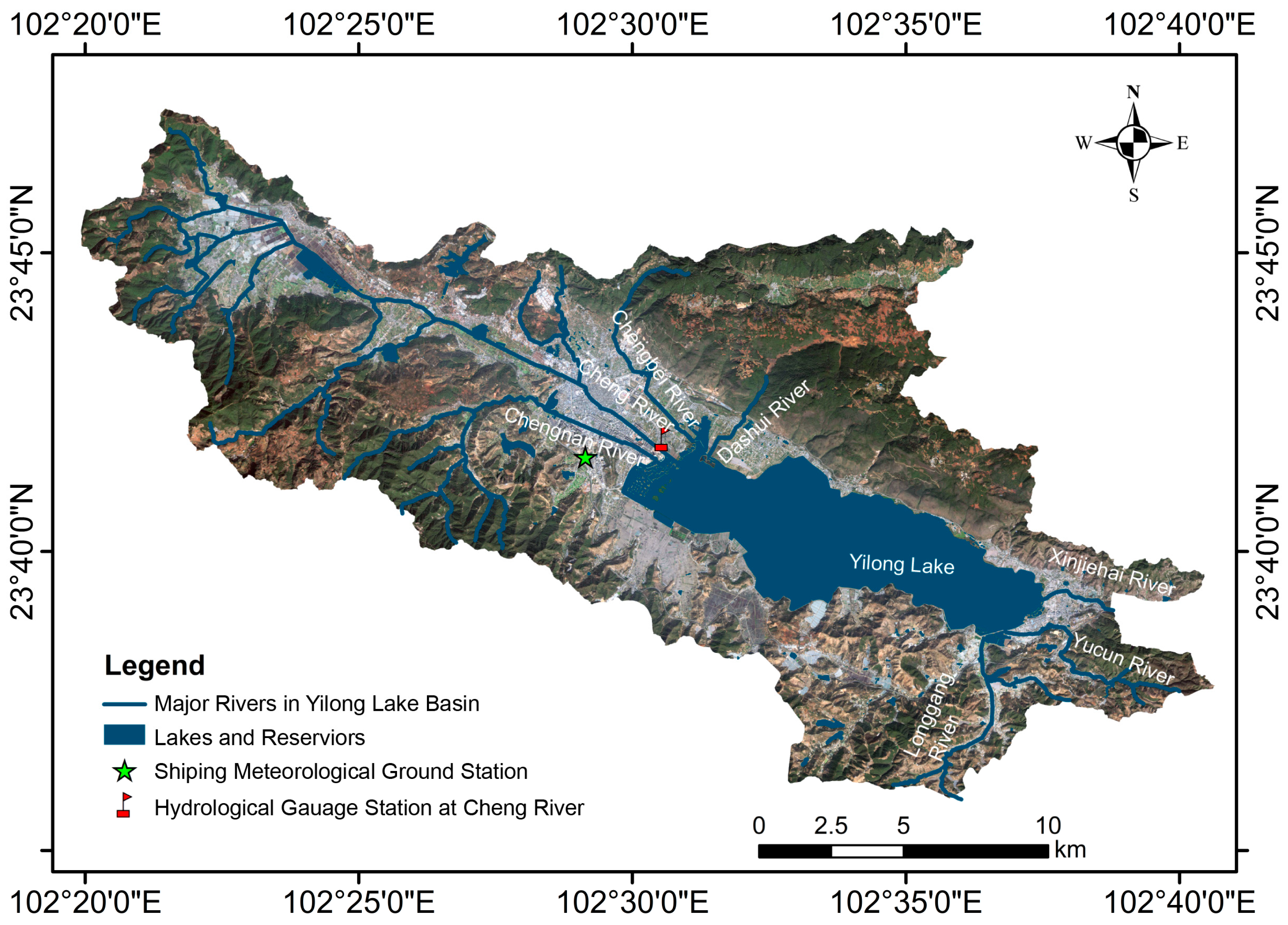
Figure 1. The location of the study area.
Water 17 01890 g001
Figure 2. A comparison of the observation and the bias-corrected downscaled GCM outputs, including the (a) daily precipitation, (b) daily mean temperature, (c) daily maximum temperature, and (d) daily minimum temperature during 2000–2014 in the YLB with a Taylor diagram.
Water 17 01890 g002
Figure 3. The study framework.
Water 17 01890 g003
Figure 4. Spatial distribution of (a) elevation, (b) slope, (c) soil types, (d) subbasins, and land use in (e) 2010 and (f) 2020 in YLB.
Water 17 01890 g004
Figure 5. The time series of observed and simulated monthly streamflows during the calibration period (2009–2017) and the validation period (2018).
Water 17 01890 g005
Figure 6. A comparison of the areal proportion of major land use types in subbasins of the YLB between the land use conditions of 2010 (left) and 2020 (right). FL, GL, FR, GR, WR, UU, and UR refer to farmland, garden land, forest, grassland, water, unused land, and urban, respectively.
Water 17 01890 g006
Figure 7. Land use transitions in (a) YLB and subbasins include (b) BASP, (c) CBH, (d) CH, (e) CNH, (f) LGH, (g) DSH, (h) NASP, (i) XJHH, and (j) YCH from 2010 to 2020. FL, GL, FR, GR, WR, UU, and UR refer to farmland, garden land, forest, grassland, water, unused land, and urban, respectively.
Water 17 01890 g007
Figure 8. Simulated streamflow and annual rainfall depth according to LC2010 and LC2020.
Water 17 01890 g008
Figure 9. Simulated time series of monthly streamflow in subbasins of (a) BASP, (b) CBH, (c) CH, (d) CNH, (e) DSH, (f) LGH, (g) NASP, (h) YCH, (i) XJHH, and (j) YLB under land use patterns of LU2010 and LU2020, respectively. Simulated streamflows with LU2010 are presented as black solid line, and simulated streamflows with LU2020 are presented as red solid line.
Water 17 01890 g009
Figure 10. Relative changes in monthly streamflow in subbasins according to LUCC from 2010 to 2020.
Water 17 01890 g010
Figure 11. Statistics of the temporal variation in the annual precipitation of four GCMs (ACCESS-CM2, ACCESS-ESM1.5, BCC-CSM2-MR, and NorESM2-LM) under different SSP scenarios (SSP245, SSP370, and SSP585).
Water 17 01890 g011
Figure 12. Time series of projected annual streamflow from 2001 to 2060 according to varied climate inputs scenarios of (a) SSP245, (b) SSP370, and (c) SSP585.
Water 17 01890 g012
Figure 13. Statistics of the temporal variation in the projected streamflow regarding four GCMs (ACCESS-CM2, ACCESS-ESM1.5, BCC-CSM2-MR, and NorESM2-LM) under different SSP scenarios (SSP245, SSP370, and SSP585).
Water 17 01890 g013
Figure 14. The relative change in the streamflow according to the reference period regarding the GCMs with different SSP scenarios. (a) ACCESS-CM2, (b) ACCESS-ESM1.5, (c) BCC-CSM2-MR, and (d) NorESM2-LM.
Water 17 01890 g014
Figure 15. Monthly distribution of streamflow in reference period (2001–2014) and future periods (2015–2030, 2031–2045, and 2046–2060) according to GCMs and SSP scenarios.
Water 17 01890 g015
Table 1. Reclassification of land use/land cover types for SWAT modeling.
Land Use/Land Cover Categories in Data SourceLand Use Types Defined in Data SourceLand Use Types Defined in SWAT Model
CodesTypesCodesSWAT LULC Description
Farmland011paddy fieldRICErice
012irrigated fieldCANAspring canola, argentine
013non-irrigated fieldCORNcorn
Garden land021orchardORCDorchard
022tea gardenORCDorchard
023other gardenORCDorchard
Forest031woodlandPINEpine
032shrub landRNGBrange, brush
033other forestFRSDforest, deciduous
Grassland043other grassHAYhay
Transportation101railway landUTRNtransportation
102highway landUTRNtransportation
104rural roadsUTRNtransportation
Water and utilities111riverWATRwater
112lakeWATRwater
113reservoirWATRwater
114pondWATRwater
116tidal flatWATRwater
117ditchWATRwater
118hydraulic construction landUINSinstitutional
Other122facility agricultural landUINSinstitutional
127barrenBARRbarren
Residential land202townURMDresidential medium density
203villageURLDresidential low density
Mining land204mining landUIDUindustrial
Public administration and public service land205scenic spots and special sitesUINSinstitutional
Table 2. Information about the global climate models whose outputs were used in this study.
No.ModelDeveloped CountryResolution
1ACCESS-CM2Australia1.875° × 1.25°
2ACCESS-ESM1.5Australia1.875° × 1.25°
3BCC-CSM2-MRChina1.1250° × 1.1250°
4NorESM2-LMNorway1.0° × 1.0°
Table 3. The data description applied in this study.
Data TypeData PeriodResolution/ScaleData SourceReferences
dem-2.5 m
(grid)
multi-source remote sensing image fusionYunnan Geological Data Center
land cover/land use data20101:10,000the 2nd national land resource survey with correctionYunnan Geological Data Center
20201:5000the 3rd national land resource survey with correction
soil data-1000 m
(grid)
Chinese Soil Dataset based on the World Soil Database (HWSD) (v1.1)National Cryosphere Desert Data Center
(https://www.ncdc.ac.cn/portal/metadata/a948627d-4b71-4f68-b1b6-fe02e302af09, accessed on 10 April 2022)
historical meteorological data (precipitation, average temperature, maximum temperature, and minimum temperature)1990–2020dailyShiping Meteorological Ground StationMeteorological Bureau of Shiping County
projected meteorological data (daily humidity, daily precipitation, daily averaged surface wind speed, daily mean temperature, daily maximum temperature, and daily minimum temperature)2000–2060dailyNEX-GDDP-CMIP6 datasetNASA Center for Climate Simulation
(https://www.nccs.nasa.gov/services/data-collections/land-based-products/nex-gddp-cmip6, accessed on 8 May 2024)
historical streamflow data2009–2018monthlyCheng River (CR) gauge stationShiping Water Authority
water system’s shape file (major reservoirs, ponds, and ditches)--local surveyYunnan Geological Data Center
Table 4. A summary of the calibrated parameters using the SWAT-CUP program in this study.
Parameterp-Valuet-StatMethodInitial RangeFitted Value
R_CN2.mgt0.0026.879R_relative−0.5…0.5−0.23
V_ALPH_BF.gw0.008−3.480V_replace0…10.21
V_GW_DELAY.gw0.0701.871V_replace30…300172
V_GWQMN.gw0.8820.164V_replace0…53.63
V_GW_REVAP.gw0.853−0.230V_replace0.02…0.20.145
V_ESCO.hru0.534−0.591V_replace0…0.50.028
V_CH_N2.rte0.0272.298V_replace0…0.30.134
V_CH_K2.rte0.4830.722V_replace5…200187
R_SOL_AWC.sol0.0701.904R_relative0…10.41
R_SOL_K.sol0.4370.821R_relative0…30.97
V_SURLAG.bsn0.1931.313V_replace0.05…2420.36
R_SOL_Z.sol0.5760.558R_relative−0.5…54.13
V_EPCO.hru0.1471.445R_relative−0.5…0.5−0.29
Notes: R_relative: parameter value is multiplied by (1 + given value); V_replace: parameter value is replaced by given value.
Table 5. Statistic characteristics of future temperatures of GCMs. CV refers to coefficient of variation.
GCMsStatistic IndexesSSP245SSP370SSP585
ACCESS-CM2Mean value (°C)9.799.899.95
Trend (°C/year)+0.043+0.054+0.044
Standard deviation (°C)0.680.710.88
Coefficient of variation0.070.070.09
ACCESS-ESM1.5Mean value (°C)9.749.6210.01
Trend (°C/year)+0.040+0.060+0.045
Standard deviation (°C)0.620.740.89
Coefficient of variation0.060.080.09
BCC-CSM2-MRMean value (°C)9.229.289.35
Trend (°C/year)+0.035+0.046+0.040
Standard deviation (°C)0.550.600.68
Coefficient of variation0.060.060.07
NorESM2-LMMean value (°C)8.778.669.09
Trend (°C/year)+0.025+0.034+0.022
Standard deviation (°C)0.600.540.75
Coefficient of variation0.070.060.08
Table 6. Statistic characteristics of future precipitations of GCMs in 2000–2060.
GCMsStatistic IndexesSSP245SSP370SSP585
ACCESS-CM2Mean value (mm/year)109310691098
Trend (mm/year)+1.912−1.093−1.24
Standard deviation (mm)112103128
Coefficient of variation0.100.100.12
ACCESS-ESM1.5Mean value (mm/year)10589991030
Trend (mm/year)+1.617+0.014−1.54
Standard deviation (mm)145128162
Coefficient of variation0.140.130.16
BCC-CSM2-MRMean value (mm/year)105810371089
Trend (mm/year)+1.641+0.582−0.38
Standard deviation (mm)98108124
Coefficient of variation0.090.100.11
NorESM2-LMMean value (mm/year)108011041082
Trend (mm/year)+0.012−0.564−0.60
Standard deviation (mm)141167162
Coefficient of variation0.130.150.15
Table 7. The monotonic trend test of projected annual streamflows with the Mann–Kendall test. The notation ↑ refers to an increasing trend, ↓ refers to a decreasing trend, and - refers to no trend.
SSPGCMs2001–20602015–20302031–20452046–2060
ZcpTrendZcpTrendZcpTrendZcpTrend
SSP245ACCESS-CM21.970.051.580.11-0.890.37-−1.390.17-
ACCESS-ESM1.50.520.60-−1.170.24-0.001.00-1.980.05
BCC-CSM2-MR0.430.66-−0.540.59-0.001.00-−1.980.05
NorESM2-LM1.200.23-1.130.26-0.001.00-−0.790.43-
Ensemble1.420.16-0.450.65-0.200.84-−0.450.66-
SSP370ACCESS-CM20.940.35-1.670.10−0.590.55-−0.400.69-
ACCESS-ESM1.5−0.960.34-−0.050.96-−0.740.46-0.690.49-
BCC-CSM2-MR−1.820.070.810.42-−1.190.24-0.250.80-
NorESM2-LM−0.930.36-0.950.34-−1.980.05−0.500.62-
Ensemble−0.400.16-1.440.15-−2.330.020.150.88-
SSP585ACCESS-CM20.610.55-0.680.50-1.930.05−1.390.17-
ACCESS-ESM1.5−0.230.82-−1.350.18-−0.990.32-−0.890.37-
BCC-CSM2-MR0.460.65-3.110.000.050.96-1.240.22-
NorESM2-LM−0.960.34-−1.670.101.540.13-1.730.08
Ensemble−0.370.71-0.630.53-1.980.05−0.100.92-
Disclaimer/Publisher’s Note: The statements, opinions and data contained in all publications are solely those of the individual author(s) and contributor(s) and not of MDPI and/or the editor(s). MDPI and/or the editor(s) disclaim responsibility for any injury to people or property resulting from any ideas, methods, instructions or products referred to in the content.