Article

Flood Exposure Patterns Induced by Sea Level Rise in Coastal Urban Areas of Europe and North Africa

1
Institute of Technology and Life Sciences—National Research Institute, Falenty, Al. Hrabska 3, 05-090 Raszyn, Poland
2
Department of Ecology, Climatology and Air Protection, Faculty of Environmental Engineering and Land Surveying, University of Agriculture in Krakow, Mickiewicza 21, 31-120 Kraków, Poland
*
Author to whom correspondence should be addressed.
Water 2025, 17(13), 1889; https://doi.org/10.3390/w17131889
Submission received: 29 April 2025 / Revised: 23 June 2025 / Accepted: 23 June 2025 / Published: 25 June 2025
(This article belongs to the Section Oceans and Coastal Zones)

Abstract

Coastal cities and low-lying areas are increasingly vulnerable, and accurate data is needed to identify where interventions are most required. We compared 53 cities affected by a 1 m increase in land levels and a 2 m rise in sea levels. The geographical scope of this study covered selected coastal cities in Europe and northern Africa. Data were sourced from the European Environment Agency (EEA) in the form of prepared datasets, which were further processed for analysis. Statistical methods were applied to compare the extent of urban flooding under two sea level rise scenarios—1 m and 2 m—by calculating the percentage of affected urban areas. To assess social vulnerability, the analysis included several variables: MAPF65 (Mean Area Potentially Flooded for people aged 65 and older, indicating elderly exposure), Age (the percentage of the population aged 65+ in each city), MAPF (Mean Area Potentially Flooded, representing the average share of urban area at risk of flooding), and Unemployment Ratio (the percentage of unemployed individuals living in the areas potentially affected by sea level rise). We utilized t-tests to analyze the means of two datasets, yielding a mean difference of 2.9536. Both parametric and bootstrap confidence intervals included zero, and the p-values from the t-tests (0.289 and 0.289) indicated no statistically significant difference between the means. The Bayes factor (0.178) provided substantial evidence supporting equal means, while Cohen’s D (0.099) indicated a very small effect size. Ceuta’s flooding value (502.8) was identified as a significant outlier (p < 0.05), indicating high flood risk. A Grubbs’ test confirmed Ceuta as a significant outlier. A Wilcoxon test highlighted significant deviations between the medians, with a p << 0.001, demonstrating systematic discrepancies tied to flood frequency and sea level anomalies. These findings illuminated critical disparities in flooding trends across specific locations, offering essential insights for urban planning and mitigation strategies in cities vulnerable to rising sea levels and extreme weather patterns. Information on coastal flooding provides awareness of how rising sea levels affect at-risk areas. Examining factors such as MAPF and population data enables the detection of the most threatened zones and supports targeted action. These perceptions are essential for strengthening climate resilience, improving emergency planning, and directing resources where they are needed most.

Graphical Abstract

1. Introduction

Recently, cities have become increasingly vulnerable due to heavy rainfall, with coastal cities being particularly at risk of flooding [1,2]. These cities face additional threats such as storm surges [3]. In France, flood risk management is supported by Caisse Centrale de Réassurance (CCR), which develops tools to estimate exposure to climatic risks such as floods. These tools use stochastic methods and climate models, such as ARPEGE-Climate, to simulate the potential losses from extreme events, considering factors like rainfall, sea level rise, and demographic growth. Projections show that losses will increase by 2050 due to both climate factors and population growth in flood-prone areas [4]. The DANA effect impacts regions such as the Mar Menor lagoon in Spain, where flooding events in 2016 and 2019 altered oceanographic properties. Extreme weather events, intensified by climate change, alter seawater parameters and demand the management of natural and human impacts [5]. In Europe, flood risk assessment relies on probability (H), consequences (C), and vulnerability (V), using data from sources like Munich Re NatCatSERVICE (a global database of natural disasters providing data on the occurrence and impact of events like floods, storms, and earthquakes). It is widely used for risk analysis and climate research used to catalog flood losses [6]. The projected rise in sea levels along the Catalan coast by 2100 ranges from 0.53 m to 1.75 m, depending on the scenario [7]. This poses a significant threat to Mediterranean regions as well as areas with colder seas along Europe’s coastal zones. The level of development along coastal zones further reduces beaches’ natural resilience to sea level rise, with limited space for adaptation [8]. As a result, the lack of accommodation space will be a factor contributing to the severity of the impacts on the region’s coastal ecosystems and infrastructure [9]. By 2100, extreme sea levels (ESLs) along European coasts are projected to rise by 57 cm under RCP (Representative Concentration Pathway) 4.5 and 1 m under RCP 8.5. The North Sea will experience the highest increase, followed by the Baltic Sea and the United Kingdom and Ireland’s Atlantic coasts. Rising sea levels (RSLR) will be the main driver, with storm surges and waves amplifying the effects in northern Europe. In southern Europe, reductions in surge and wave extremes may partially offset RSLR. By the end of the century, 5 million Europeans could face annual coastal flooding under high-end warming [10].
One of the negative phenomena exacerbated by extreme weather events is the DANA (Depresión Aislada en Niveles Altos) effect, which causes intense and destructive rainfall. Recently, such an event was recorded in the southern part of Spain, leading to catastrophic consequences for coastal infrastructure [11]. Given this, it is crucial to study the level of urbanization and the degree of land sealing in urban areas. Attention should be paid to the location of infrastructure both in the city center and outside the main urban areas to assess the so-called “urban sprawl” effect [12]. Urban sprawl refers to the uneven distribution of urban infrastructure, including buildings, roads, and bridges, which extends beyond a city’s administrative boundaries. This can increase the risk of flooding in these areas [13]. This trend is particularly relevant for larger cities, as decentralization is linked to cities with a higher degree of urbanization. It may also be associated with economic zones located outside cities. With urbanization, access to the coastline increases in many countries, and the process leads to a concentration of population in coastal areas. This is particularly evident in China. As a result, more people are living in areas vulnerable to climate-change-related risks, particularly flooding and sea level rise, which increases the exposure of these regions to such threats [14]. Cities such as Odense, Vienna, Strasbourg, and Nice face significant flood risks due to both urban development and climate change. The extent of these risks varies: climate change is the primary factor in Nice, while urban development plays a more substantial role in Strasbourg [15].
The growth of coastal tourism increases vulnerability to flooding, yet existing models overlook its impact on casualty calculations, as demonstrated by a Belgian case study showing the need to consider tourism dynamics in flood risk management [16]. Small islands focused on coastal tourism, such as Tenerife and Gran Canaria, are highly vulnerable to marine storms. A recent study [17] identified 144 storm episodes in Tenerife and 154 in Gran Canaria between 1958 and 2017, and highlighted that the storms damaged local infrastructure, led to beach erosion, and resulted in loss of life. A study on an extreme wind event in an Italian alpine region revealed a 17–23% drop in summer tourism over 2–3 years in the most affected areas, particularly those with fewer cultural assets and less foreign tourism, highlighting the sector’s past vulnerability and the need for preventive policies [18]. Another study examined the spatiotemporal variability of extreme wave storms around the Canary Archipelago, focusing on Tenerife’s southern coast, and revealed complex spatial patterns, seasonal variability, and significant impacts on beaches and infrastructure, including a case of severe erosion. Another study examined the spatiotemporal variability of extreme wave storms around the Canary Archipelago, focusing on Tenerife’s southern coast, and revealed complex spatial patterns, seasonal variability, and significant impacts on beaches and infrastructure, including a case of severe erosion [19]. In various regions around the world, the threat of rising sea levels is becoming increasingly evident—for example, in Cape Town [20] and Accra, Ghana [21], as well as in the Caribbean region [22]. Moreover, it is increasingly observed and projected that the infrastructure of coastal cities may be at risk due to sea level rise, with European coastal cities also facing threats from storm surges. In this text, GDP (gross domestic product) represents the total value of goods and services produced in a region, used to assess the economic impact of climate change, such as sea level rise and tourism shifts [23]. Because storm waves threaten the coastlines of France, the United Kingdom, Portugal, and Italy, various measures and geoengineering tools should be employed to protect critical infrastructure [24]. The need to study coastal cities is being acknowledged both by local authorities and within the scientific community, as coastal areas are home to a large share of the population [25,26,27,28,29]. Therefore, actions should already be taken to prepare for potential relocations, particularly affecting elderly residents over the age of 65 [30].
This research addresses an important gap: the lack of integration between flood risk models and social data for people aged 65 and older. This is particularly problematic given that we are living in an aging society. Flood risk models typically focus on physical exposure to hazards, but they often overlook critical social factors such as demographics and socioeconomic conditions. Integrating these social elements is essential to fully understand how flooding impacts coastal communities and their capacity to respond effectively. Therefore, the objectives of the paper are as follows:
(a) To assess the risk relationship in European and North African coastal cities within administrative areas (core cities based on the Urban Morphological Zones dataset);
(b) To evaluate the dataset showing the percentage of cities inundated by a 1 m rise in sea level and to assess the consequences, including the impacts of 1 m and 2 m sea-level rise flooding;
(c) To explore the relationship using principal component analysis based on area flooded and the interaction between social factors and flood exposure.

2. Materials and Methods

2.1. Data on European and North African Cities

Materials were sourced from the database of the European Environment Agency [31]. These data are publicly accessible and can be downloaded from the agency’s website. There are no restrictions on obtaining or disseminating these data. They pertain to coastal cities in Europe and North Africa. The first group was related to climate modeling concerning a sea level rise of 1 m. The second group was associated with modeling and a sea level rise of 2 m. The analysis estimated the percentage of the administrative areas of European coastal cities inundated by a 1 m and 2 m sea-level rise, using the Urban Morphological Zones dataset and elevation data from the 2018 CReSIS (Centre for Remote Sensing of Ice Sheets) dataset. GIS (geographic information system) tools overlaid sea level projections onto city boundaries, assuming no coastal defenses, to compute the proportion of inundated land. Data on the frequency of extreme weather events according to RCP 4.5—Representative Concentration Pathway scenarios, covering the years 2010 to 2100—was obtained from the European Environment Agency [32]. Using national-level demographic indicators for city-level analysis is a limitation because such data may not accurately reflect local population characteristics. Cities can have very different age structures, employment rates, or socioeconomic conditions compared to the national average. This discrepancy can lead to less precise assessments of vulnerability or exposure on the urban scale.

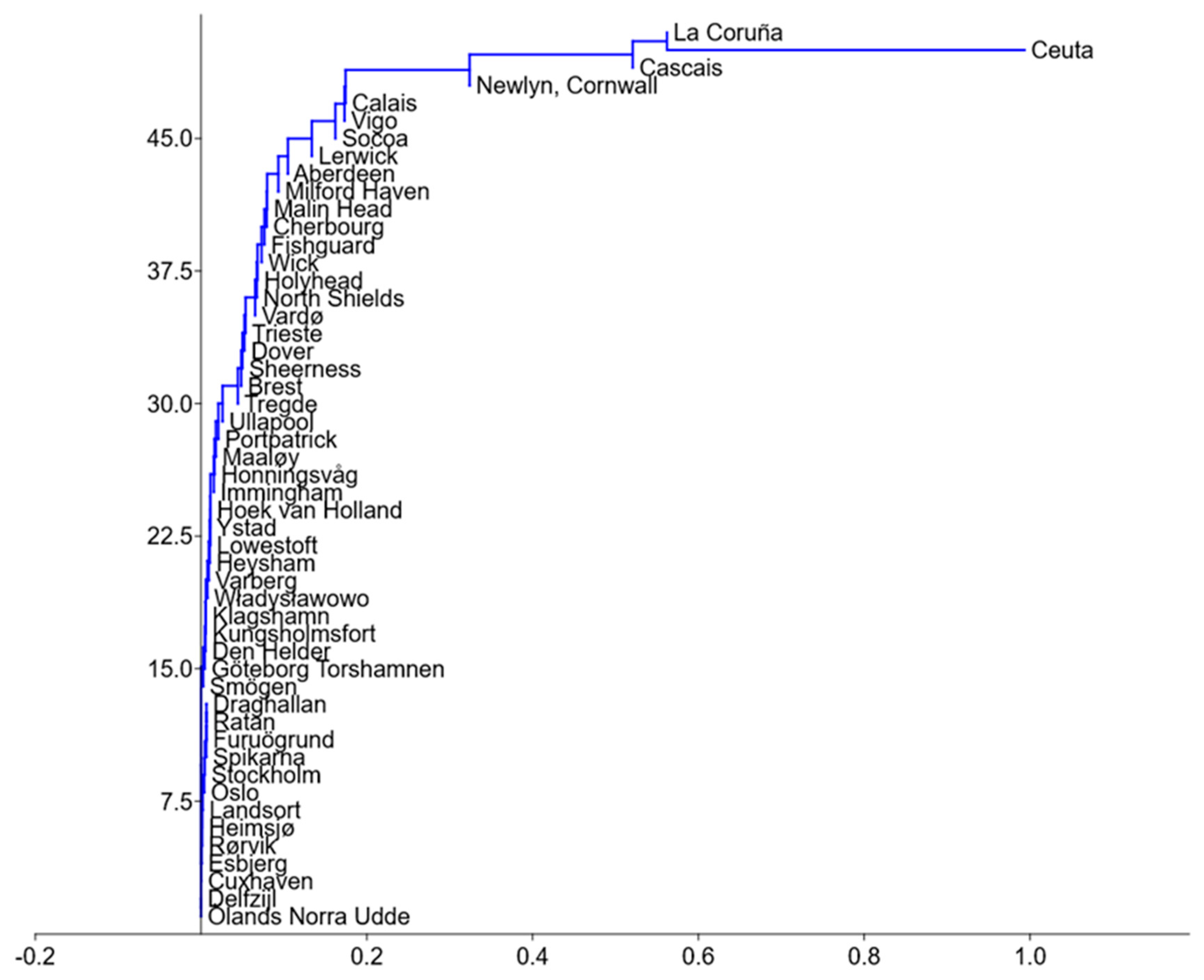
2.2. Statistical Analysis of Cities Prone to Sea Storm Flooding

The provided data was analyzed to identify relationships between flood frequency and statistical thresholds by comparing observed R values with critical thresholds (Rcrit); cities where R > Rcrit were flagged as outliers, indicating extreme flooding risks. The top 20% most extreme flooding frequencies were highlighted for detailed analysis. The normality of residuals was tested using four methods: D’Agostino–Pearson (p = 0.1666) and Shapiro–Wilk (p = 0.0584) confirmed a normal distribution, while Anderson–Darling (p = 0.0134) and Kolmogorov–Smirnov (p = 0.0254) showed deviations, indicating mixed results regarding normality.
Cities were categorized based on the estimated multiplication factor of flooding events due to projected sea level rise. This categorization divides cities into clear risk levels, offering a systematic way to assess and prioritize flood mitigation efforts. Low-risk cities (<10) are those with minimal projected increases in flooding, while medium-risk cities (10–50) face moderate increases. High-risk locations (50–100) are expected to encounter significant rises in flood frequency, whereas extreme-risk cities (>100) are the most vulnerable, requiring urgent attention and mitigation strategies. Flood frequency data from sea level rise events was sourced, including values for each city, statistical measures (R), critical thresholds (Rcrit), and identification of outliers. R values were compared to Rcrit at a significance level of p < 0.05:
  • If R > Rcrit, the city was marked as an outlier;
  • If R ≤ Rcrit, the city was not considered an outlier.
In the analysis, several statistical tests were performed to investigate variability, outliers, and differences in central tendencies. A Grubbs’ test was conducted to identify outliers, successfully flagging significant deviations in the dataset.
To compare the effects of 1 m and 2 m sea level rise scenarios, a Wilcoxon signed-rank test was used. This nonparametric test evaluates whether the median difference between paired observations significantly deviates from zero. The test was chosen because it does not assume normality, is robust to outliers, and is well-suited for skewed environmental or socioeconomic data. When exact p-values were not feasible, normal approximation was applied. Additionally, Z-test and t-test methodologies were utilized to compare the sample means with hypothesized values, evaluating significance and providing confidence intervals.
To compare the effects of 1 m and 2 m rises in sea levels, t-tests for equal means were conducted. The tests evaluated differences in the central tendencies between two datasets: one representing a 1 m rise and the other a 2 m rise. Both parametric and bootstrap methods were used to calculate confidence intervals for the difference between the means. Monte Carlo permutation tests provided additional verification of the results, while effect sizes were measured using Cohen’s D. The analysis also calculated Bayes factors to assess the strength of evidence for the hypothesis of equal means.
A Fligner–Killeen test was performed to assess the equality of the coefficients of variation between the two datasets representing a 1 m rise and a 2 m rise in sea levels.
An Epps–Singleton test was applied to assess whether the two datasets shared identical distributions. This nonparametric test is particularly useful for comparing empirical distributions without relying heavily on assumptions about the underlying data.
A Mood’s test for equal medians was carried out to examine whether the medians of the two datasets were statistically equivalent. This test evaluates differences in medians by analyzing dispersion in the data, supplemented by a Fisher’s exact test for additional robustness.
A Mann–Whitney test and Brunner–Munzel test were employed to examine the stochastic equality between the two datasets. The Mann–Whitney test was used to compare the 1 m and 2 m sea level rise scenarios by evaluating whether the distributions of variables differ significantly between the two. This test is appropriate because it does not require normally distributed data and works well with skewed or ordinal data. In contrast, the Brunner–Munzel test was used to assess probabilistic dominance between the groups, and it is particularly useful when the two groups have unequal variances. The data of coastal cities was analyzed using PaSt version 4.17, applying statistical methods to evaluate the relationships between variables and flooding risks [33].

2.3. National Level Data for At-Risk Groups in Coastal Flooded Areas

The analysis investigated the following variables: MAPF65, Age, MAPF, and Unemployment Ratio.
MAPF65 represents Mean Area Periodically Flooded for people aged 65 and older in flooded areas. It indicates the average extent of periodically flooded zones inhabited by elderly residents in coastal cities.
Age represents the percentage of the population aged 65 and older in coastal cities. This variable reflects the demographic aging of populations living in areas vulnerable to sea level rise.
MAPF stands for the Mean Area Potentially Flooded in coastal cities. It measures the average size of areas at risk of flooding due to rising sea levels.
Unemployment Ratio is defined as the percentage of unemployed individuals in flooded areas of cities affected by rising sea levels.
This variable highlights the socioeconomic vulnerability of populations living in flood-prone zones. Multiple regression analysis and variance inflation factor (VIF) assessments were conducted to evaluate multicollinearity among factors such as MAPF, Age, and Unemployment Ratio. Principal component analysis (PCA) was performed to identify patterns and summarize variance in the dataset. This analysis was executed using GraphPad Prism 10.0, which enabled robust regression modeling, detailed ANOVA testing, and normality assessments. These methods provided precise insights into the relationships between flooding risks, affected populations (particularly elderly individuals), and contributing factors, ensuring a comprehensive understanding of the impacts of rising sea levels on coastal cities.
The methodology for creating a hypothetical Markov chain transition matrix based on static data involved initially defining discrete states of flood risk: Low (MAPF < 5), Medium (5 ≤ MAPF < 10), and High (MAPF ≥ 10). Subsequently, each unit (country) from the provided dataset was assigned to one of these states based on its MAPF value at a given point in time. The next step was establishing hypothetical transition probabilities between these states over a presumed time period, where these probabilities did not directly stem from the data but were arbitrary assumptions regarding the dynamics of risk change. Finally, these hypothetical probabilities were placed into a transition matrix, with each element representing the probability of transitioning from a starting state (row) to an ending state (column) in a single time step, which allowed for an illustrative modeling of potential future states of the system under the assumption that the process adheres to the properties of a Markov chain. It was assumed how a region might transition between flood potential states over a certain time frame (a year). These probabilities were hypothetical. The flood risk transition dynamics can be represented using a probabilistic state transition matrix where cities shift between three risk categories: Low (L), Medium (M), and High (H). A city currently at the Low risk has a 70% chance of remaining Low, a 20% chance of increasing to Medium, and a 10% chance of escalating to High. For cities at the Medium risk, there’s a 30% probability of improvement to Low, a 50% chance of stability, and a 20% risk of escalation. High-risk cities face a 5% chance of significant improvement to Low, a 35% chance of moderating to Medium, and a 60% likelihood of remaining at High. This matrix structure is typical in logistic or Markov-based risk modeling and captures both the persistence and mobility of flood exposure levels over time.

3. Results

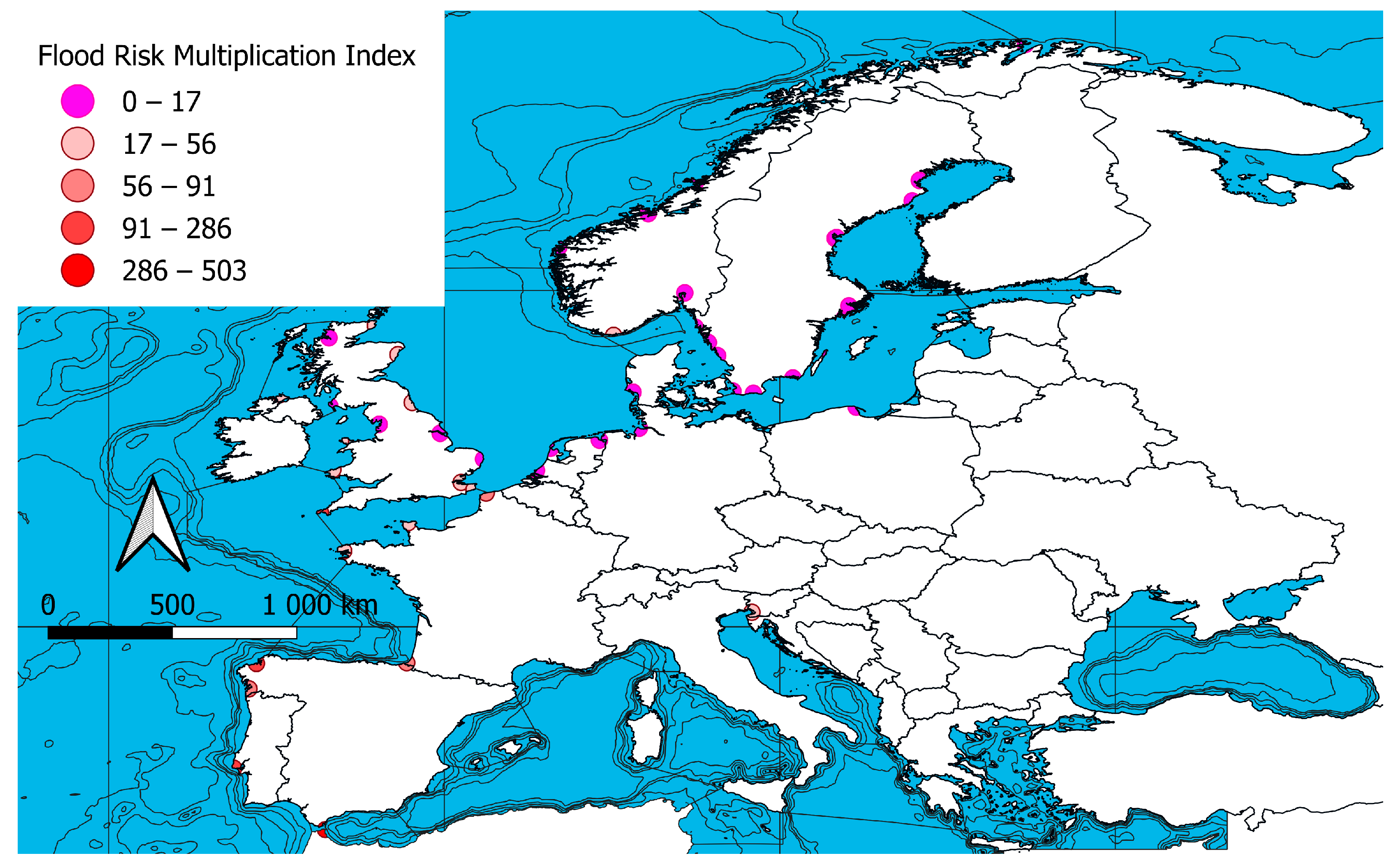
3.1. Storm Risk in European and North African Coastal Cities

The Wilcoxon test for a single sample was applied to examine differences in the medians. The given median of 0 was compared against the sample median of 11.6, yielding a test statistic (W) of 1326. The normal approximation produced a z-value of 6.2148, with a p-value < 0.001. Since the p-value is extremely small, this strongly suggests that the medians differ significantly. The sample mean was reported as 44.218, and the results include both a Z-test and a t-test. In the Z-test, the test statistic was −0.50458, with a p-value (two-tailed) of 0.61385, while the t-test yielded a statistic of −0.49971 and a similar p-value of 0.61947. Both p-values are much greater than the typical significance threshold of 0.05, indicating that the observed sample mean does not significantly differ from the hypothesized population mean. Residuals passed the normality tests, including D’Agostino–Pearson and Shapiro–Wilk, but deviations observed in the Anderson–Darling and Kolmogorov–Smirnov tests suggested that the model’s assumptions require cautious evaluation.
The Mann–Whitney U test showed a small difference in the ranks between cities exposed to a 1 m and 2 m rise, with a U-statistic of 23.56 and a z-statistic of 1.8693. However, the p-value (0.061586) and the Monte Carlo p-value (0.0647) indicated that this difference was not statistically significant, as both values were slightly above the typical significance threshold of 0.05. The effect size (Vargha–Delaney A = 0.4495) suggested a small effect, indicating a slight preference for larger values in the 2 m rise group. Similarly, the Brunner–Munzel test provided a p-value of 0.06123 and a Monte Carlo p-value of 0.0643, which further supported the finding that the distributions of the two groups were not significantly different. The degrees of freedom for the Brunner–Munzel test were 447.71, reinforcing the consistency across tests. Overall, the results did not provide strong evidence of a significant difference between cities exposed to a 1 m and 2 m sea level rise (Table 1).
The statistical analysis comparing cities exposed to a 1 m and 2 m sea level rise indicated no significant difference in the distributions of the two groups. The Mood’s test (Chi2 = 1.258, p = 0.261) and the W test (W = 3.121, p = 0.537) both suggested that the distributions were not significantly different. The Fligner–Killeen test showed a slight difference in the coefficients of variation (CVs), with the 1 m rise having a higher CV (156.71) compared to the 2 m rise (143.49), but the two-tailed p-value (0.062) was marginally above the significance threshold, indicating no strong evidence of a difference. The z-value of 1.866 and the p-value of 0.031 in the one-tailed test suggested a potential difference, but the overall results did not support a statistically significant divergence between the two scenarios (Table 2).
The comparison between cities exposed to 1 m and 2 m sea level rise showed that although the mean flood-prone area was slightly higher for the 2 m scenario, the difference was small and not statistically significant. Confidence intervals overlapped substantially, variance and standard deviations were similar, and multiple tests—including t-tests, bootstrap, and permutation—consistently supported the hypothesis of equal means. The very small effect size (Cohen’s D = 0.099) and a Bayes Factor of 0.178 further indicated negligible differences between the two scenarios (Table 3).
Socoa is a statistically significant outlier (R > Rcrit). This indicates heightened flood risks likely caused by sea level rise. These cities should be prioritized for immediate flood mitigation strategies. The dataset reveals that out of 10 cities, 7 exhibit flooding levels considered extreme (outliers). However, cities like Lerwick, Aberdeen, and Milford Haven are within expected ranges and pose lower risks based on this analysis (Table 4).
The highest frequency of multiplied phenomena was observed in cities located along the Atlantic Ocean, with the number ranging from 286 to 503. Some cities along the Baltic Sea and the North Sea had a lower flood risk. The difference between areas exposed to open ocean waters and those near enclosed seas, such as the Baltic, was found to be 4–5 times greater (Figure 1).
Along the Baltic Sea, Adriatic Sea, Tyrrhenian Sea, Aegean Sea, and Black Sea, the projected sea level rise is expected to be similar across all regions, reaching up to 20%. In urban morphological zones, the situation is likely to resemble that of Ireland and the United Kingdom. In the North Sea, particularly in the Netherlands, the rise is projected to be significantly higher, by at least 80% and potentially up to 100%. Additionally, an increased flood risk of 1 m is anticipated for Portugal (Figure 2).
Most cities are not exposed to flooding from a 2 m rise in sea level in the Baltic Sea. Only Cuxhaven in Germany has an elevated exposure in its urban morphological zone, ranging from 55% to 80%. Selected cities in Ireland and the United Kingdom also show elevated risks, with very high exposures up to 100% observed in Belgium and the Netherlands. Spain (Valencia), Portugal (Lisbon), France (Saint-Nazaire), and Italy (Trieste) also show increased exposure values (Figure 3).
Overall, most cities had similar values for the multiplication of flooding risks caused by rising sea levels and were clustered close to each other. Exceptionally, cities like Newlyn, Cornwall, Cascais, and La Coruña showed significant differences. Ceuta stood out with a separate position in the dendrogram classification (Figure 4).
The first row indicated that if a region was currently in a Low flood potential state, there was a 70% chance it would remain in that state, a 20% chance it would move to Medium, and a 10% chance it would move to High in the subsequent time period. The probabilities are as follows: from Low (L) to Low (L): 0.8, Medium (M): 0.15, High (H): 0.05; from Medium (M) to Low (L): 0.4, Medium (M): 0.4, High (H): 0.2; from High (H) to Low (L): 0.1, Medium (M): 0.5, High (H): 0.4 (Figure 5).

3.2. Results of the Socioeconomic Analysis Related to Flood-Prone Areas

MAPF was found to have the strongest impact on MAPF65 outcomes, demonstrated by a highly significant coefficient (β2 = 0.9115, p < 0.05) and low multicollinearity (VIF = 1.182), highlighting its crucial role in shaping the vulnerability of populations aged 65 and older in flooded areas. Age had a negligible effect on MAPF65, as indicated by its nonsignificant coefficient (β1 = −0.01165, p > 0.05), suggesting minimal influence from the proportion of elderly individuals. Unemployment Ratio showed weak statistical significance (β3 = −0.2882, p > 0.05) and faced multicollinearity concerns (VIF = 6.704), limiting its explanatory power. The interaction term (Age: MAPF: Unemployment Ratio) was also insignificant (β4 = 0.008471, p > 0.05), demonstrating no meaningful contribution (Table 5).
The first two principal components (PC1 and PC2) account for a significant portion of the variance: 50.33% and 41.66%, respectively. The analysis revealed that MAPF significantly influenced MAPF65, indicating that the extent of flooded areas plays a critical role in determining the vulnerability of populations aged 65 and older in affected regions. Age had a negligible effect, suggesting that the percentage of elderly individuals in coastal cities did not contribute meaningfully to the variation in MAPF65 (Figure 6).

4. Discussion

4.1. Flood Events and Storm Surges in European–Mediterranean Coastal Areas

The flood risk modeling system in France, which combines hazard, vulnerability, and damage models, has shown effective results in estimating insurance-related losses caused by coastal flooding. The model successfully predicted damage from the Xynthia storm, but its accuracy is limited by the availability of detailed data on water heights and coastal topography. This system is sensitive to these factors, suggesting that improvements in data quality could enhance its precision [34]. Our coastal cities are frequently exposed to periodic flooding (Figure 1), particularly in the Mediterranean region, with Spain and North Africa being especially vulnerable to storms. One contributing factor may be the weather effect. The DANA (Depresión Aislada en Niveles Altos) phenomenon primarily occurs in southeastern Spain, in the Region of Murcia and the Segura Basin, as evidenced during the September 2019 event [35]. The European Coastal Flood Awareness System (ECFAS) project uses a catalogue of flood maps to assess storm-related flooding along Europe’s coastline. These maps are generated from flood models based on synthetic scenarios, incorporating various storm durations and total water level (TWL) peaks. The model has been validated with observed data, showing good accuracy (over 80% hit scores in half of the test cases). It highlights that low-lying areas experience the most significant flooding, with variations based on storm duration and TWL peaks. The study also finds that urban and wetland areas influence flood extent, supporting the idea of wetland-based storm flood mitigation [36]. The results presented in this region showed that Valencia is exposed to a 25% risk of inundation (Figure 2). For the Mann–Whitney test, the mean ranks were 105.96 for the 1 m rise and 123.54 for the 2 m rise, yielding a test statistic (U) of 23,556 and a z-value of 1.8693. The associated p-value was 0.061586, with a Monte Carlo permutation p-value of 0.0647, indicating marginal significance. The Vargha–Delaney effect size was 0.4495, reflecting a small value. For the Brunner–Munzel test, the probabilistic estimate (phat) was 0.55051, with a test statistic of 1.8766 and degrees of freedom (df) of 447.71. The p-value (0.0612) and Monte Carlo permutation p-value (0.0643) indicated borderline significance (Table 1). Identifying cities with significant flood risk allowed for efficient resource allocation—outliers required stronger interventions, while others were monitored for future changes.
Cities are vulnerable to sea level rise, as historical data showed that sea levels in the Baltic Sea fluctuated significantly over the past 9000 years. In particular, sea levels in the Pomeranian Bay and Szczecin Lagoon (Poland) rose slowly over the last 5000 years, with some extreme events disrupting the regular rise. These findings indicated that the area was prone to the effects of rising sea levels, with potential impacts on coastal cities [37]. Weather phenomena, including coastal flooding, have impacted Kołobrzeg, with historical accounts recording sudden and rapid floods, such as the “Sea Bear” phenomenon. Geological data revealed evidence of two significant events (17 September 1497 and 1 March 1779), with the 1497 event leaving a sand layer approximately 10 cm thick 1400 m from the shore. This suggests a flood height of 4.9 m above sea level, likely caused by atmospheric factors that triggered wave events similar to tsunamis [38]. The Mood’s test for equal medians yielded a Chi-square statistic of 1.2585 with a p-value of 0.26193, indicating no significant difference between medians. The Fisher’s exact test confirmed this, with a p-value of 0.26191, supporting the absence of measurable disparity (Table 2). The analysis compared 223 observations for a 1 m rise and 235 for a 2 m rise in sea levels. The very small effect size (Cohen’s D = 0.09905) and substantial evidence for equal means (Bayes factor = 0.1787) suggested minimal differentiation between the impacts of a 1 m and 2 m sea level rise. The associated p-value of 0.53765 indicated no significant difference between the distributions, suggesting that the two scenarios do not exhibit statistically distinct patterns based on the observed data (Table 3).

4.2. The Impact of Storm Surges and Rising Sea Levels on the Residents of Coastal Cities

Gdańsk and Haarlem in the Netherlands have a long history, with Dutch Mennonites establishing a settlement in the Vistula delta in the 16th century. Despite extensive civil defense works, both regions have experienced significant floods, such as the Dutch southwest coast in 1953, the Rhine riverbank in 1993 and 1995, and the Vistula delta in 2001. Climate change projections show that both areas will suffer from rising sea levels and severe rainfall, with Poland and the Netherlands adopting similar approaches to address the impacts of climate change on their coastal cities [39]. Coastal cities in Poland faced a 5% flood risk for core centers within their urban morphological zones (Figure 2). In contrast, projections for sea level rise along the Danish coast indicated an increase of 0.6 to 1.2 m by the year 2120 under both low- and high-emission scenarios (SSP1-1.9 and SSP5-8.5). By that time, approximately 14% of Denmark’s coastal habitats were expected to experience permanent flooding, although only 1.6% of urban areas were projected to be affected. Without additional protective measures, about 191,000 hectares of agricultural land were expected to face frequent flooding, while 45% (199 km2) of coastal wetlands were predicted to be permanently inundated [40]. These findings underlined critical patterns in the flooding trends and deviations tied to sea level rise.
Cities identified as outliers—Ceula, La Coruña, Cascais, Newlyn, and Socoa—demonstrated statistically significant flooding frequencies, highlighting their critical vulnerability to sea level rise and the urgency of implementing interventions. Nonoutlier cities—Lerwick, Aberdeen, and Milford Haven—showed relatively stable flooding frequencies, though ongoing monitoring remained necessary. When applied, the Grubbs’ test identified 502.8 in Ceuta as a significant outlier (p < 0.05), reflecting anomalously high flooding frequencies (Table 4). Overall, Denmark showed less than a 5% flood risk with a 1 m sea level rise; however, Copenhagen alone exhibited a significantly higher risk, ranging from 10% to 25% (Figure 2). Meanwhile, Copenhagen is also exposed to a projected 2 m sea level rise, which is on a similar risk level (Figure 3). On the other hand, cities such as Venice in Italy are exposed to a sea level rise of at least 2 m, with a 50% risk. Coastal areas in Italy exhibit varying subsidence rates, with the Volturno River mouth showing moderate subsidence (−2.5 to −7.5 mm/y) and higher rates in back-dune depressions (−10 mm/y). The Sarno coastal plain has moderate subsidence near Castellammare di Stabia (−0.25 to −1 mm/y) and higher rates near the river mouth (−1 to −5 mm/y). The Alento Plain shows low subsidence rates in the north (−1.9 to −0.3 mm/y) and a hot spot up to −3 mm/y inland. The RCP8.5 scenario for 2065 and 2100 assesses around 180 km2 in Volturno, 8.5 km2 in Sarno, 60 km2 in Sele, and 7 km2 in Alento Plain [41].
During storm Xaver, the sea level on the German coast reached a record high due to a combination of high surges, mean sea level, and high tides. The peak of the storm resulted in a sea level rise that was simulated to occur at the maximum water level, which was about 1 m higher than normal, particularly in Cuxhaven. Coastal defenses, including sea dikes 6–9.5 m above sea level, prevented most potential damage. A scenario with a 1 m height increase was also considered for flood adaptation [42].
The results indicated that in countries/areas such as Belgium, the Netherlands, the Spanish coast, one city in Germany (Cuxhaven), and Lisbon in Portugal, urban morphological zones are exposed to a 2 m inundation risk at levels of at least 50% (Figure 3). In Belgium, storm forecasting in areas such as the Ardennes and cities is possible through the use of regional climate models, such as MAR (Modèle Atmosphérique Régional, a regional atmospheric model), which simulate future scenarios based on NorESM1-M and MIROC5 (climate models used to simulate climate changes on a global scale), under RCP 8.5 (Representative Concentration Pathway 8.5, a climate change scenario assuming a high level of greenhouse gas emissions leading to a significant rise in global temperatures). After assessing their accuracy in representing the current climate, these models show that by the end of the century, the snow depletion process is likely to accelerate, reducing the risk of snowmelt-related floods. However, no significant change was found in the frequency of extreme precipitation events, although these trends are subject to uncertainties due to model physics and natural variability [43].

4.3. Social and Economic Factors of Potentially Flooded Areas

The effectiveness of land use policies in mitigating coastal flood risks in the waterfront areas of Helsinki and Espoo, Finland, was shown as a solution to storm surge issues. The study found that municipal land use policies were highly effective in relocating vulnerable land use types outside sea flood risk zones, with land use conversions between 2000 and 2018 showing positive results. These conversions were classified into two groups: desirable land use changes, such as conversions from artificial surfaces to other types or from agricultural areas to non-artificial surfaces. Natural areas and wetlands were considered less vulnerable to flooding, and the framework allowed for flexibility in classifying land use conversions based on its objectives, enhancing its functional capability [44]. Age and MAPF were identified as predictors in the multiple regression model and should be regarded as critical factors in future assessments (Table 5). The PCA results revealed urban areas potentially exposed to flooding, alongside indicators such as unemployment rates and population aging. The analysis showed that aging has a significant impact on labor market supply. People aged 65 and older were found to predominantly reside in areas with high potential flood risk (Figure 6). The plot presented a principal component analysis that visualized relationships between the variables influencing flood risk in coastal cities. The first two components (PC1 and PC2) together explained over 90% of the data variance (50.33% and 41.66%, respectively). The arrows (vectors) indicated the strength and direction of each variable’s contribution—longer vectors represented a stronger influence. Data points were color-coded by PC1 values, which revealed patterns related to Mean Area Potentially Flooded, MAPF65 (Flooded areas affecting people aged 65+), Age (percentage of population aged 65+), and Unemployment Ratio (percentage of unemployed individuals in flood-prone areas) (Figure 6). The PCA indicated that older age and unemployment are factors contributing to increased flood vulnerability, with most of the variance explained by these socioeconomic elements and sea level rise.
Based on the analysis of maps depicting coastal cities in Europe, it can be concluded that cities located within the Baltic Sea basin are less exposed to flooding risks compared to those situated in the North Sea basin (Figure 1). This is supported by findings from the Netherlands, where sea level rise poses significant risks. However, with strategies such as Protect, Advance, and Accommodate, a livable future remains possible—even with a projected 5 m rise. Achieving this requires substantial investment in infrastructure, land use modifications, and cross-sectoral adaptation efforts [45].
The neighbor cluster joining analysis revealed that most cities could be grouped into common clusters. Ceuta emerged as an extreme outlier, while cities such as Newlyn, Cornwall, Cascais, and La Coruña formed a distinct group of storm-prone urban areas (Figure 4). The study revealed varying levels of exposure, showing that cities are not equally vulnerable to sea level rise. While regional trends differed, common patterns emerged; for instance, Władysławowo (Baltic) was classified as low risk, Dover (North Sea) as medium risk, and Vigo (Mediterranean) as high risk.
Furthermore, the Markov chain probability analysis showed that the highest likelihood of transition was from Low to Medium (0.2), while the probability of a city moving from High to Low was very low (0.05). A more probable shift was from High to Medium (0.35), as illustrated in the diagram of coastal cities classified by storm frequency exposure (Figure 5).
Similarly, Unemployment Ratio showed weak statistical significance and faced multicollinearity issues, limiting its role in explaining MAPF65. The interaction term combining Age, MAPF, and Unemployment Ratio was also insignificant, confirming no meaningful combined effects on MAPF65. The findings highlighted the importance of focusing resources and interventions on reducing the extent of flooded areas to protect at-risk populations, particularly the elderly, in coastal cities impacted by rising sea levels. The regression model proved robust, with an R-squared value of 0.9585, effectively capturing most variability in MAPF65, confirming MAPF as the dominant predictive factor. The analysis found that only Mean Area Potentially Flooded significantly influenced flood outcomes, with larger areas linked to higher impacts. In contrast, Age and Unemployment Ratio had no significant individual effects, as their confidence intervals included zero. The three-way interaction between Age, MAPF, and Unemployment Ratio also did not show a meaningful impact (Table 5).

5. Conclusions

This paper identified Ceuta, La Coruña, Cascais, Newlyn, Cornwall, Calais, Vigo, Socoa, Lerwick, Aberdeen, and Milford Haven as the top 20% of cities most exposed to coastal flooding. Among them, Ceuta, La Coruña, Cascais, Newlyn, and Socoa were statistically significant outliers (R > Rcrit), indicating heightened flood risks associated with rising sea levels and possible data anomalies. These results indicated discrepancies in measurements, which may reflect significant patterns or anomalies tied to sea level variations and flooding risk. These cities require immediate flood mitigation strategies to protect vulnerable populations, particularly those aged 65 and older. Out of the 10 cities analyzed, 7 exhibited extreme flooding risks. MAPF, representing flooded coastal areas, was confirmed as the strongest influence on Mean Area Periodically Flooded for individuals aged 65 and older in these regions, emphasizing its critical role in shaping vulnerability. Other factors, such as Age and Unemployment Ratio, showed limited impacts on MAPF65, with some multicollinearity concerns. The PCA analysis further highlighted how MAPF predominantly explained the observed variance in the dataset. These findings stress the urgency of targeted interventions to mitigate flooding in high-risk areas while maintaining vigilant monitoring in lower-risk regions. The analysis highlighted the need to address flooding risks, particularly for vulnerable elderly populations in affected regions. Age and unemployment rate had little impact, but monitoring these factors along with flooded areas remains important. Efforts should focus on flood prevention and mitigation in high-risk areas to protect those most at risk.

Author Contributions

Conceptualization, W.H.; methodology, W.H.; software, W.H.; validation, D.B.; data curation, W.H.; writing—original draft preparation, W.H. and D.B.; writing—review and editing, D.B. and W.H.; visualization, W.H.; funding acquisition, W.H. All authors have read and agreed to the published version of the manuscript.

Funding

This research received no external funding.

Data Availability Statement

Data will be provided upon request.

Conflicts of Interest

The authors declare no conflicts of interest.

References

  1. Prokic, M.N.; Savić, S.; Pavić, D. Pluvial flooding in urban areas across the European continent. Geogr. Pannonica 2019, 23, 216–232. [Google Scholar] [CrossRef]
  2. Laino, E.; Iglesias, G. Beyond coastal hazards: A comprehensive methodology for the assessment of climate-related hazards in European coastal cities. Ocean Coast. Manag. 2024, 257, 107343. [Google Scholar] [CrossRef]
  3. Bevacqua, E.; Maraun, D.; Vousdoukas, M.I.; Voukouvalas, E.; Vrac, M.; Mentaschi, L.; Widmann, M. Higher probability of compound flooding from precipitation and storm surge in Europe under anthropogenic climate change. Sci. Adv. 2019, 5, eaaw5531. [Google Scholar] [CrossRef] [PubMed]
  4. Moncoulon, D.; Veysseire, M.; Naulin, J.P.; Wang, Z.X.; Tinard, P.; Desarthe, J.; Déqué, M. Modelling the evolution of the financial impacts of flood and storm surge between 2015 and 2050 in France. Int. J. Saf. Secur. Eng. 2016, 6, 141–149. [Google Scholar] [CrossRef]
  5. Machado Toffolo, M.; Grilli, F.; Prandi, C.; Goffredo, S.; Marini, M. Extreme Flooding Events in Coastal Lagoons: Seawater Parameters and Rainfall over A Six-Year Period in the Mar Menor (SE Spain). J. Mar. Sci. Eng. 2022, 10, 1521. [Google Scholar] [CrossRef]
  6. Kron, W.; Löw, P.; Kundzewicz, Z.W. Changes in risk of extreme weather events in Europe. Environ. Sci. Policy 2019, 100, 74–83. [Google Scholar] [CrossRef]
  7. Jiménez, J.A.; Valdemoro, H.I.; Bosom, E.; Sánchez-Arcilla, A.; Nicholls, R.J. Impacts of sea-level rise-induced erosion on the Catalan coast. Reg. Environ. Chang. 2017, 17, 593–603. [Google Scholar] [CrossRef]
  8. Brunel, C.; Sabatier, F. Potential influence of sea-level rise in controlling shoreline position on the French Mediterranean Coast. Geomorphology 2009, 107, 47–57. [Google Scholar] [CrossRef]
  9. Sierra, J.P.; Casanovas, I.; Mösso, C.; Mestres, M.; Sanchez-Arcilla, A. Vulnerability of Catalan (NW Mediterranean) ports to wave overtopping due to different scenarios of sea level rise. Reg. Environ. Change 2016, 16, 1457–1468. [Google Scholar] [CrossRef]
  10. Vousdoukas, M.I.; Mentaschi, L.; Voukouvalas, E.; Verlaan, M.; Feyen, L. Extreme sea levels on the rise along Europe’s coasts. Earth’s Future 2017, 5, 304–323. [Google Scholar] [CrossRef]
  11. Eguibar, M.Á.; Porta-García, R.; Torrijo, F.J.; Garzón-Roca, J. Flood Hazards in Flat Coastal Areas of the Eastern Iberian Peninsula: A Case Study in Oliva (Valencia, Spain). Water 2021, 13, 2975. [Google Scholar] [CrossRef]
  12. Xu, L.; Cui, S.; Wang, X.; Tang, J.; Nitivattananon, V.; Ding, S.; Nguyen, M.N. Dynamic risk of coastal flood and driving factors: Integrating local sea level rise and spatially explicit urban growth. J. Clean. Prod. 2021, 321, 129039. [Google Scholar] [CrossRef]
  13. Zhao, Q.; Pepe, A.; Devlin, A.; Zhang, S.; Falabella, F.; Zeni, G.; Pan, J. Impact of sea-level-rise and human activities in coastal regions: An overview. J. Geod. Geoinf. Sci. 2021, 4, 124. [Google Scholar]
  14. McGranahan, G.; Balk, D.; Anderson, B. The rising tide: Assessing the risks of climate change and human settlements in low elevation coastal zones. Environ. Urban. 2007, 19, 17–37. [Google Scholar] [CrossRef]
  15. Skougaard Kaspersen, P.; Høegh Ravn, N.; Arnbjerg-Nielsen, K.; Madsen, H.; Drews, M. Comparison of the impacts of urban development and climate change on exposing European cities to pluvial flooding. Hydrol. Earth Syst. Sci. 2017, 21, 4131–4147. [Google Scholar] [CrossRef]
  16. Kellens, W.; Neutens, T.; Deckers, P.; Reyns, J.; De Maeyer, P. Coastal flood risks and seasonal tourism: Analysing the effects of tourism dynamics on casualty calculations. Nat. Hazards 2012, 60, 1211–1229. [Google Scholar] [CrossRef]
  17. Yanes Luque, A.; Rodríguez-Báez, J.A.; Máyer Suárez, P.; Dorta Antequera, P.; López-Díez, A.; Díaz-Pacheco, J.; Pérez-Chacón, E. Marine storms in coastal tourist areas of the Canary Islands. Nat. Hazards 2021, 109, 1297–1325. [Google Scholar] [CrossRef]
  18. Bernardi, M.; Cascarano, M.; Modena, F. Weathering the storm: The impact of the Vaia storm on tourism flows. Clim. Change 2025, 178, 20. [Google Scholar] [CrossRef]
  19. Guerra-Medina, D.; Rodríguez, G. Spatiotemporal variability of extreme wave storms in a beach tourism destination area. Geosciences 2021, 11, 237. [Google Scholar] [CrossRef]
  20. Dube, K.; Nhamo, G.; Chikodzi, D. Rising sea level and its implications on coastal tourism development in Cape Town, South Africa. J. Outdoor Recreat. Tour. 2021, 33, 100346. [Google Scholar] [CrossRef]
  21. Sagoe-Addy, K.; Appeaning Addo, K. Effect of predicted sea level rise on tourism facilities along Ghana’s Accra coast. J. Coast. Conserv. 2013, 17, 155–166. [Google Scholar] [CrossRef]
  22. Scott, D.; Simpson, M.C.; Sim, R. The vulnerability of Caribbean coastal tourism to scenarios of climate change related sea level rise. J. Sustain. Tour. 2012, 20, 883–898. [Google Scholar] [CrossRef]
  23. Bigano, A.; Bosello, F.; Roson, R.; Tol, R.S. Economy-wide impacts of climate change: A joint analysis for sea level rise and tourism. Mitig. Adapt. Strateg. Glob. Change 2008, 13, 765–791. [Google Scholar] [CrossRef]
  24. Garnier, E.; Ciavola, P.; Spencer, T.; Ferreira, O.; Armaroli, C.; Mcivor, A. Historical analysis of storm events: Case studies in France, England, Portugal and Italy. Coast. Eng. 2018, 134, 10–23. [Google Scholar] [CrossRef]
  25. Laino, E.; Iglesias, G. Extreme climate change hazards and impacts on European coastal cities: A Review. Renew. Sustain. Energy Rev. 2023, 184, 113587. [Google Scholar] [CrossRef]
  26. McDonagh, B.; Worthen, H.; Mottram, S. Governing flood risk in mid seventeenth-century England. J. Hist. Geogr. 2025, 89, 13–26. [Google Scholar] [CrossRef]
  27. Mirto, A.P.M.; Vacca, D.; Martina, L.; Mistretta, A.; Olla, E.; Rizzo, F.P. Modelling Population and Health Profiles in Italian and European Coastal and non-Coastal Areas. Soc. Indic. Res. 2025, 1–27. [Google Scholar] [CrossRef]
  28. Gonçalves, C.; Pinho, P. The governance of the coastal region: Evolutionary changes in the conceptualisation and integration of landscape in Portuguese coastal planning institutions. Landsc. Ecol. 2025, 40, 1–28. [Google Scholar] [CrossRef]
  29. Vinet, F.; Lumbroso, D.; Defossez, S.; Boissier, L. A comparative analysis of the loss of life during two recent floods in France: The sea surge caused by the storm Xynthia and the flash flood in Var. Nat. Hazards 2012, 61, 1179–1201. [Google Scholar] [CrossRef]
  30. Bukvic, A.; Gohlke, J.; Borate, A.; Suggs, J. Aging in flood-prone coastal areas: Discerning the health and well-being risk for older residents. Int. J. Environ. Res. Public Health 2018, 15, 2900. [Google Scholar] [CrossRef]
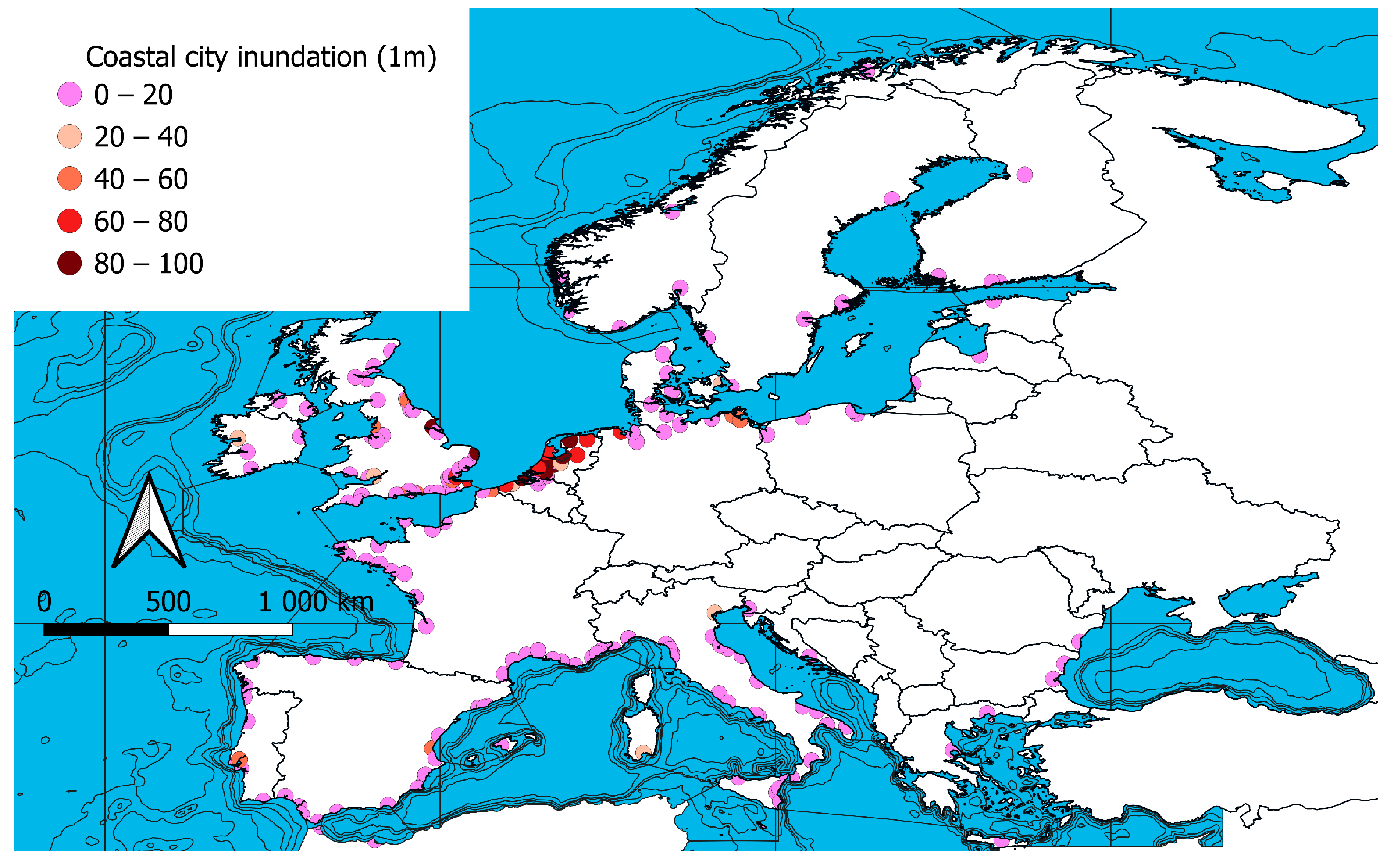
  31. European Environment Agency. Area Inundated with 2m Sea Level Rise, Jan. 2020. Available online: https://sdi.eea.europa.eu/catalogue/srv/api/records/d96b007a-4e26-4dbd-8dd5-24dbe5c9b31f (accessed on 15 April 2025).
  32. European Environment Agency. Change in the Frequency of Flooding Events Under Projected Sea Level Rise (RCP 4.5; Change Between 2010 and 2100; Multiplication Factor), Dec. 2016. 2016. Available online: https://sdi.eea.europa.eu/catalogue/srv/api/records/723f0742-727b-45ec-a70d-df6292b7e003 (accessed on 15 April 2025).
  33. Hammer, Ø.; Harper, D.A. Past: Paleontological statistics software package for education and data analysis. Palaeontol. Electron. 2001, 4, 1. [Google Scholar]
  34. Naulin, J.P.; Moncoulon, D.; Le Roy, S.; Pedreros, R.; Idier, D.; Oliveros, C. Estimation of insurance-related losses resulting from coastal flooding in France. Nat. Hazards Earth Syst. Sci. 2016, 16, 195–207. [Google Scholar] [CrossRef]
  35. Romero-Díaz, M.A.; Morales, A.P. Before, during and after the Dana of September 2019 in the region of Murcia (Spain), as reported in the written press. Cuad. Investig. Geogr. 2021, 47, 163–182. [Google Scholar] [CrossRef]
  36. Le Gal, M.; Fernández-Montblanc, T.; Duo, E.; Montes Perez, J.; Cabrita, P.; Souto Ceccon, P.; Armaroli, C. A new European coastal flood database for low–medium intensity events. Nat. Hazards Earth Syst. Sci. 2023, 23, 3585–3602. [Google Scholar] [CrossRef]
  37. Sydor, P.; Uścinowicz, S. Holocene relative sea-level changes in the eastern part of Pomeranian Bay and the Szczecin Lagoon, Southern Baltic Sea. Holocene 2022, 32, 351–368. [Google Scholar] [CrossRef]
  38. Piotrowski, A.; Brose, F.; Sydor, P. Coastal flooding in Kołobrzeg (Kolberg) area, southern Baltic Sea, in the light of historical and geological data. Holocene 2024, 34, 1721–1732. [Google Scholar] [CrossRef]
  39. Sanders, F.; Sanders, H.; Jonkers, K. Cross-over analysis of the climate-change delta situation of the cities Gdansk (Baltic-sea) and Rotterdam (Nord-sea). Open Res. Eur. 2021, 1, 9. [Google Scholar] [CrossRef]
  40. Canal-Vergés, P.; Frederiksen, L.; Egemose, S.; Ebbensgaard, T.; Laustsen, K.; Flindt, M.R. Impacts of Sea Level Rise on Danish Coastal Wetlands–A GIS-based Analysis. Environ. Manag. 2024, 75, 1039–1054. [Google Scholar] [CrossRef]
  41. Di Paola, G.; Rizzo, A.; Benassai, G.; Corrado, G.; Matano, F.; Aucelli, P.P. Sea-level rise impact and future scenarios of inundation risk along the coastal plains in Campania (Italy). Environ. Earth Sci. 2021, 80, 608. [Google Scholar] [CrossRef]
  42. Koks, E.E.; Le Bars, D.; Essenfelder, A.H.; Nirandjan, S.; Sayers, P. The impacts of coastal flooding and sea level rise on critical infrastructure: A novel storyline approach. Sustain. Resil. Infrastruct. 2023, 8 (Suppl. S1), 237–261. [Google Scholar] [CrossRef]
  43. Wyard, C.; Scholzen, C.; Doutreloup, S.; Hallot, É.; Fettweis, X. Future evolution of the hydroclimatic conditions favouring floods in the south-east of Belgium by 2100 using a regional climate model. Int. J. Climatol. 2021, 41, 647–662. [Google Scholar] [CrossRef]
  44. Amani Fard, F.; Riekkinen, K.; Pellikka, H. Evaluating the Effectiveness of Land-Use Policies in Preventing the Risk of Coastal Flooding: Coastal Regions of Helsinki and Espoo. Land 2023, 12, 1631. [Google Scholar] [CrossRef]
  45. van Alphen, J.; van der Biezen, S.; Bouw, M.; Hekman, A.; Kolen, B.; Steijn, R.; Zanting, H.A. Room for Sea-Level Rise: Conceptual Perspectives to Keep The Netherlands Safe and Livable in the Long Term as Sea Level Rises. Water 2025, 17, 437. [Google Scholar] [CrossRef]
Figure 1. The index of the multiplicity of flood-prone areas in selected coastal cities.
Water 17 01889 g001
Figure 2. Selected coastal cities exposed to flooding from a 1 m sea level rise.
Water 17 01889 g002
Figure 3. Selected coastal cities exposed to flooding from a 2 m sea level rise.
Water 17 01889 g003
Figure 4. Neighbor-joining clustering using the Gower distance method for all storm-prone cities studied. The blue line represents a classification tree cluster connecting cities with similar characteristics.
Water 17 01889 g004
Figure 5. Markov chain diagram for transition states (Low—group of cities classified as having low storm exposure frequency, Medium—intermediate category, and High—cities with a high level of storm exposure) in coastal areas. Blue arrows represent transitions between different states.
Water 17 01889 g005
Figure 6. PCA biplot of factors influencing flood risk in coastal cities. Data points are color-coded based on PC1 values, revealing patterns across MAPF (Mean Area Potentially Flooded), MAPF65 (Flooded areas affecting people aged 65+), Age (percentage of the population aged 65+), and Unemployment Ratio (percentage of unemployed individuals in flooded areas). Blue arrows represent variable contributions: direction shows correlation, length indicates strength, and angle reflects relationships between variables.
Water 17 01889 g006
Table 1. Comparison of cities exposed to 1 m and 2 m sea level rise: Mann–Whitney and Brunner–Munzel tests.
Metric1 m Rise 2 m Rise StatisticValueInterpretation
Sample size (N)223235--
Mean rank105.96123.54--
Mann–Whitney U test--U23,56
z-statistic---1.8693
p-value---0.061586
Monte Carlo p-value---0.0647
Effect size (Vargha–Delaney A)--Effect Size (A)0.4495Small (slight preference for 2 m values being larger)
Brunner–Munzel test--phat0.55051
BM statistic---1.8766
Degrees of freedom---447.71
p-value---0.06123
Monte Carlo p-value---0.0643
Table 2. Comparison of cities exposed to 1 m and 2 m sea level rise.
TestMetric1 m Rise 2 m Rise StatisticValueAdditional Info
Mood’s testSample size (N)223235Chi21.258
p (same median) 0.261Fisher’s exact p = 0.261
W test (distributions)Sample size (N)223235W3.121p (same dist.) = 0.537
Distributions are not significantly different
Fligner–Killeen testSample size (N)223235CV156.71143.49
95% Confidence interval(138.01, 173.13)(127.7, 157.43)T246.48Expected T = 219.37
z 1.866
p (one-tailed) 0.031
p (two-tailed) 0.062
Notes: CV (Coefficient of variation): A measure of relative dispersion around the mean, expressed as a percentage. Higher CV values indicate greater variability in the data. T: Test statistic used in the Fligner–Killeen test for comparing coefficients of variation. Expected T: The expected value of the test statistic under the null hypothesis of equal variances. z: Standardized test result, showing the difference between observed and expected values in terms of standard deviations. p (one-tailed): The p-value for a one-tailed test, assessing whether one variable is significantly larger or smaller than the other. p (two-tailed): The p-value for a two-tailed test, evaluating whether there is any difference between variables (either greater or smaller). Chi2 (Chi-square): Test statistic used in the Mood’s test to assess the equality of medians. W: Test statistic used to compare distributions in the W test (distribution equality test).
Table 3. Comparative analysis for cities exposed to 1 m and 2 m sea level rise using statistics and parameters.
Metric1 m Rise 2 m Rise Statistic/ParameterValueComments
Sample size (N)223235 Larger sample size for 2 m rise
Mean area18,43121,384 Higher mean area for 2 m rise
95% Confidence interval(14,619; 22,242)(17,441; 25,328) Overlapping intervals indicate similarity
Variance834.17941.49 Slightly higher variance for 2 m rise
Difference of means 2.953 Small difference between means
95% CI (parametric) (−2.5249; 8.432) Indicates substantial overlap
95% CI (bootstrap) (−2.5193; 8.452) Similar findings via bootstrap method
t-statistic (equal variances) 1.059Supports evidence for equal means
p-value (equal variances) 0.289Not statistically significant
t-statistic (unequal variances) 1.061
p-value (unequal variances) 0.289Consistent with equal means evidence
Monte Carlo permutation p-value 0.291
Bayes factor 0.178Substantial evidence for equal means
Cohen’s D 0.099Very small effect size; negligible difference
Epps–Singleton test W Statistic3.12Distributions are not significantly different
Parameter typeNNMean13
Standard deviation1111 Similar dispersion for both rises
Notes: N (sample size): Number of observations used for analysis. A larger sample size improves reliability. Mean area: Average percentage area under analysis for each sea level rise scenario. 95% Confidence interval (CI): Range within which the true mean is expected to fall, with 95% confidence. Overlapping CIs suggest no significant difference. Variance: Measures the spread of data points around the mean. Higher variance indicates greater dispersion. Difference of means: Difference between the average values for the two conditions (1 m vs. 2 m rise). t-statistic: A value from t-tests assessing whether two group means are statistically different. p-value: Probability of observing the data assuming the null hypothesis is true. If p < 0.05, the result is considered statistically significant. Monte Carlo permutation p-value: Alternative method to calculate p-values based on resampling, often used for robust statistical testing. Bayes factor: Indicates the strength of evidence supporting the null hypothesis; lower values suggest weaker evidence against equality. Cohen’s D: Effect size measure describing the magnitude of mean difference. Epps–Singleton test: A test for assessing the equality of distributions using the W statistic. Standard deviation: Measures the average distance of values from the mean, providing insight into variability.
Table 4. Extreme value analysis of metrics for the top 20% of selected cities using the Grubbs’ test.
OutlierRcritRValueRow
Yes3.1365.233502.8Ceuta
Yes3.1284.256285.9La Coruña
Yes3.125.024265.2Cascais
Yes3.1124.387166.3Newlyn, Cornwall
Yes3.1032.77891Calais
Yes3.0943.05890.4Vigo
Yes3.0853.21584.9Socoa
No3.0162.93870.6Lerwick
No3.062.44456.1Aberdeen
No3.0572.29450.3Milford Haven
Table 5. Sociological parameters used in the regression: Age, Unemployment Ratio, and MAPF.
VIF95% CIStandard ErrorEstimateVariable
-−0.6531 to 2.7270.81271.037β0 (Intercept)
2.038−1.391 to 1.3680.6633−0.01165β1 (Age)
1.1820.8179 to 1.0050.045010.9115β2 (MAPF)
6.704−1.460 to 0.88330.5633−0.2882β3 (Unemployment Ratio)
7.0−0.04919 to 0.066130.027730.008471β4 (Age: MAPF: Unemployment)
Disclaimer/Publisher’s Note: The statements, opinions and data contained in all publications are solely those of the individual author(s) and contributor(s) and not of MDPI and/or the editor(s). MDPI and/or the editor(s) disclaim responsibility for any injury to people or property resulting from any ideas, methods, instructions or products referred to in the content.

