
Comparative Analysis of Machine/Deep Learning Models for Single-Step and Multi-Step Forecasting in River Water Quality Time Series


Abstract
1. Introduction
2. Study Framework
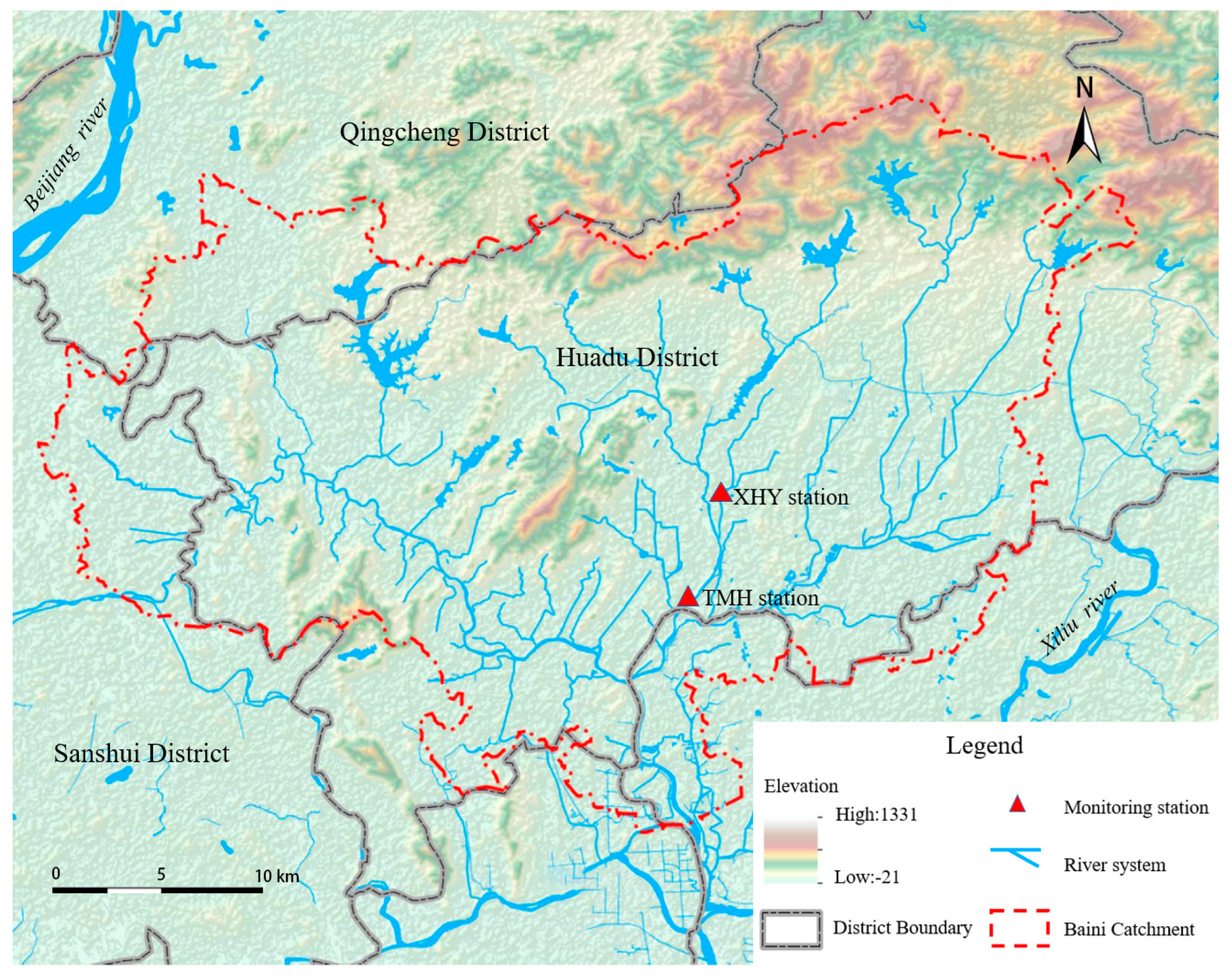
2.1. Study Area
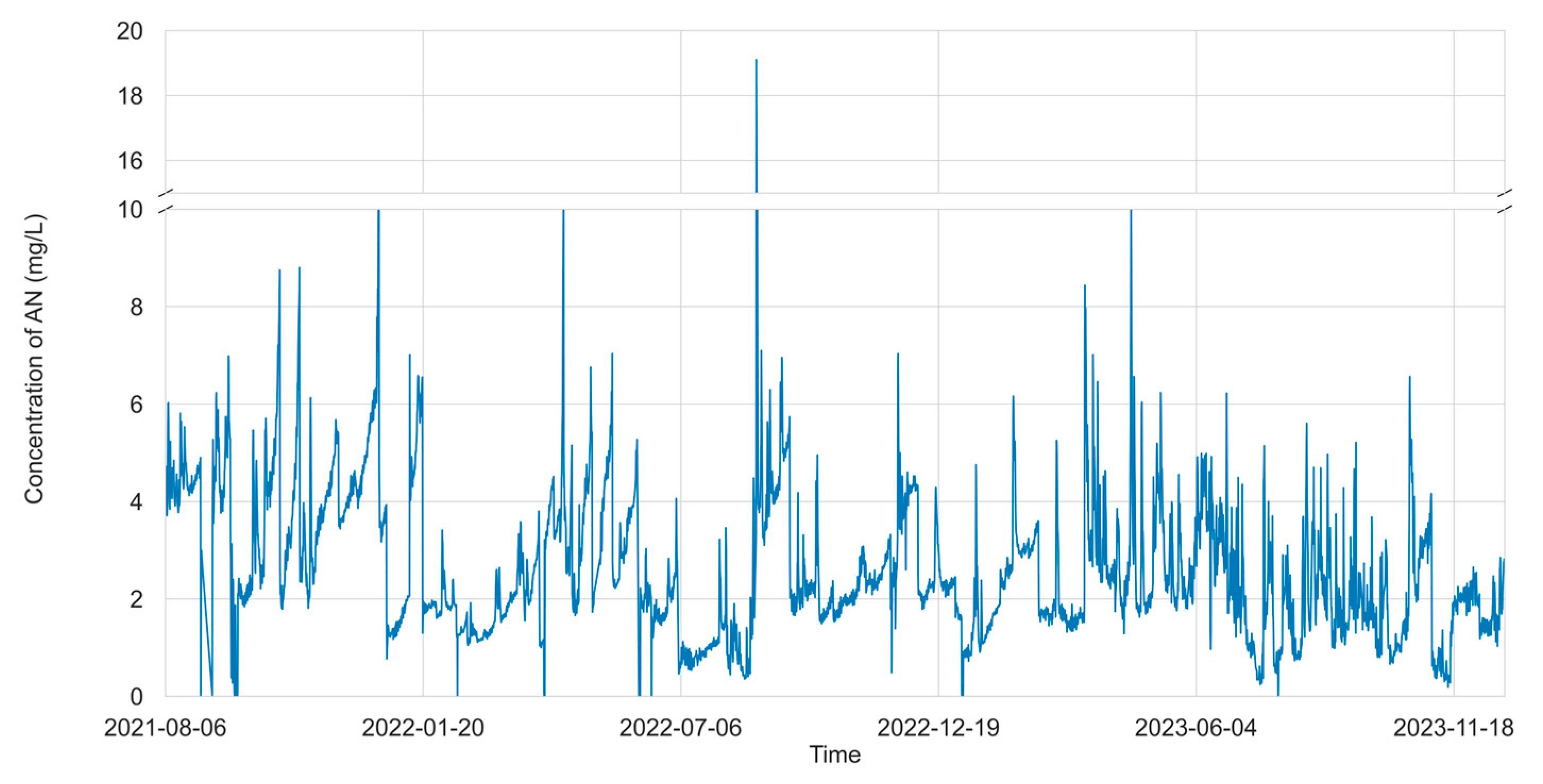
2.2. Data Preprocessing and Description
2.3. Machine/Deep Learning Models
2.3.1. Machine Learning Models
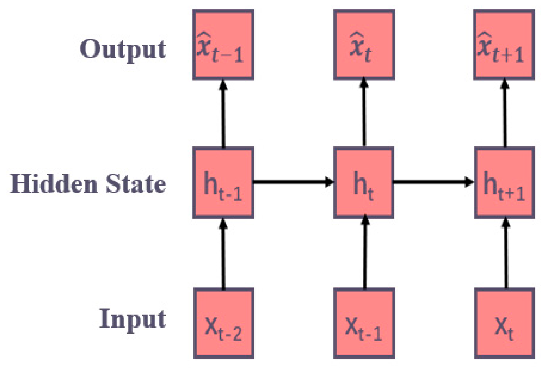
2.3.2. Deep Learning Models
2.4. Experimental Design
2.5. Model Evaluation
3. Results and Discussion
3.1. Single-Step Time Series Forecasting
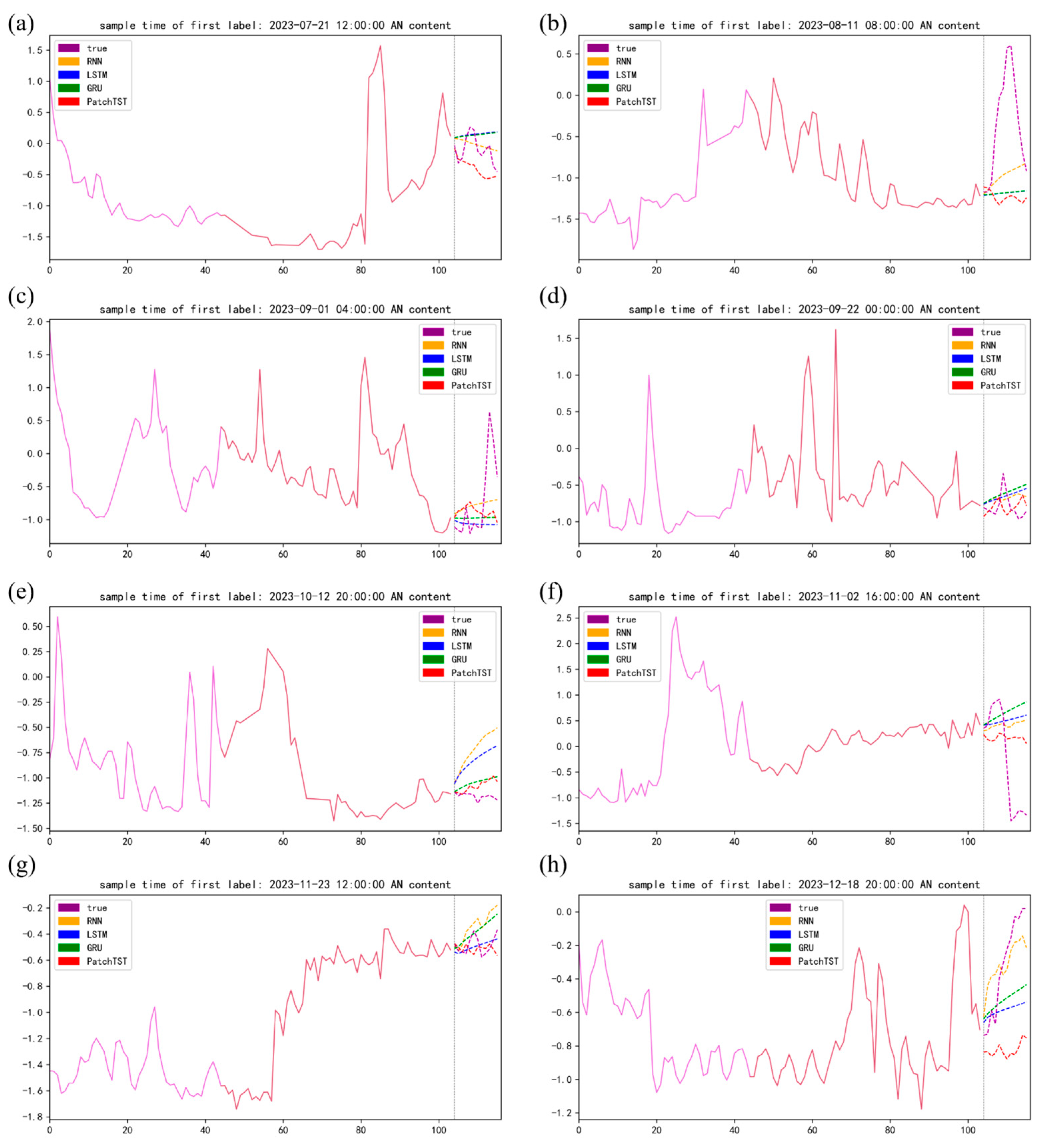
3.2. Multi-Step Time Series Forecasting
3.3. Discussion
4. Conclusions
Supplementary Materials
Author Contributions
Funding
Data Availability Statement
Conflicts of Interest
References
- Chen, K.; Chen, H.; Zhou, C.; Huang, Y.; Qi, X.; Shen, R.; Liu, F.; Zuo, M.; Zou, X.; Wang, J.; et al. Comparative analysis of surface water quality prediction performance and identification of key water parameters using different machine learning models based on big data. Water Res. 2020, 171, 115454. [Google Scholar] [CrossRef] [PubMed]
- China National Environmental Monitoring Centre. Introduction of National Surface Water Quality Automatic Monitoring System. 2017. Available online: http://www.cnemc.cn/zzjj/jcwl/shjjcwl_699/201705/t20170531_645113.shtml (accessed on 15 May 2025).
- HJ 915-2017; Technical Specifications for Automatic Monitoring of Surface Water. Ministry of Environmental Protection of the People’s Republic of China: Beijing, China, 2017.
- Gao, Z.; Chen, J.; Wang, G.; Ren, S.; Fang, L.; Yinglan, A.; Wang, Q. A novel multivariate time series prediction of crucial water quality parameters with long short-term memory (LSTM) networks. J. Contam. Hydrol. 2023, 259, 104262. [Google Scholar] [CrossRef] [PubMed]
- Gao, L.L.; Li, D.L. A review of hydrological/water-quality models. Front. Agric. Sci. Eng. 2014, 1, 267. [Google Scholar] [CrossRef]
- Charuleka, V.; Alison, P.; Appling, B.A. Can machine learning accelerate process understanding and decision-relevant predictions of river water quality? Hydrol. Process. 2022, 36, e14565. [Google Scholar]
- Wang, Y.; Yuan, Y.; Pan, Y.; Fan, Z. Modeling daily and monthly water quality indicators in a canal using a hybrid wavelet-based support vector regression structure. Water 2020, 12, 1476. [Google Scholar] [CrossRef]
- Fu, X.; Zheng, Q.; Jiang, G.; Roy, K.; Huang, L.; Liu, C.; Li, K.; Chen, H.; Song, X.; Chen, J.; et al. Water quality prediction of copper-molybdenum mining-beneficiation wastewater based on the PSO-SVR model. Front. Environ. Sci. Eng. 2023, 17, 98. [Google Scholar] [CrossRef]
- Baek, S.S.; Pyo, J.; Chun, J.A. Prediction of water level and water quality using a CNN-LSTM combined deep learning approach. Water 2020, 12, 3399. [Google Scholar] [CrossRef]
- Zhang, Y.; Li, C.; Jiang, Y.; Sun, L.; Zhao, R.; Yan, K.; Wang, W. Accurate prediction of water quality in urban drainage network with integrated EMD-LSTM model. J. Clean. Prod. 2022, 354, 131724. [Google Scholar] [CrossRef]
- Chen, L.; Wu, T.; Wang, Z.; Lin, X.; Cai, Y. A novel hybrid BPNN model based on adaptive evolutionary artificial bee colony algorithm for water quality index prediction. Ecol. Indic. 2023, 146, 109882. [Google Scholar] [CrossRef]
- Xu, J.; Wang, K.; Lin, C.; Xiao, L.; Huang, X.; Zhang, Y. FM-GRU: A time series prediction method for water quality based on seq2seq framework. Water 2021, 13, 1031. [Google Scholar] [CrossRef]
- Vaswani, A. Attention is all you need. Adv. Neural Inf. Process. Syst. 2017, 30, 5998–6008. [Google Scholar]
- Zhou, H.; Zhang, S.; Peng, J.; Zhang, S.; Li, J.; Xiong, H.; Zhang, W. Informer: Beyond efficient transformer for long sequence time-series forecasting. Proc. AAAI Conf. Artif. Intell. 2021, 35, 11106–11115. [Google Scholar] [CrossRef]
- Wu, H.; Xu, J.; Wang, J.; Long, M. Autoformer: Decomposition transformers with auto-correlation for long-term series forecasting. Adv. Neural Inf. Process. Syst. 2021, 34, 22419–22430. [Google Scholar]
- Zhou, T.; Ma, Z.; Wen, Q.; Wang, X.; Sun, L.; Jin, R. Fedformer: Frequency enhanced decomposed transformer for long-term series forecasting. Int. Conf. Mach. Learn. 2022, 162, 27268–27286. [Google Scholar]
- Zeng, A.; Chen, M.; Zhang, L.; Xu, Q. Are transformers effective for time series forecasting? Proc. AAAI Conf. Artif. Intell. 2023, 37, 11121–11128. [Google Scholar] [CrossRef]
- Lin, Y.; Qiao, J.; Bi, J.; Yuan, H.; Wang, M.; Zhang, J.; Zhou, M. Transformer-based water quality forecasting with dual patch and trend decomposition. IEEE Internet Things J. 2024, 12, 10987–10997. [Google Scholar] [CrossRef]
- Yao, S.; Zhang, Y.; Wang, P.; Xu, Z.; Wang, Y.; Zhang, Y. Long-term water quality prediction using integrated water quality indices and advanced deep learning models: A case study of Chaohu Lake, China, 2019–2022. Appl. Sci. 2022, 12, 11329. [Google Scholar] [CrossRef]
- Bi, J.; Chen, D.; Yuan, H. Graph attention transformer with dilated causal convolution and Laplacian eigenvectors for long-term water quality prediction. In Proceedings of the 2024 IEEE International Conference on Systems, Man, and Cybernetics (SMC), Sarawak, Malaysia, 6–10 October 2024; pp. 3571–3576. [Google Scholar]
- Jaffar, A.; Thamrin, N.M.; Megat, M.S.A. Water quality prediction using LSTM-RNN: A review. J. Sustain. Sci. Manag. 2022, 17, 204–225. [Google Scholar] [CrossRef]
- Liu, Y.J. Prediction of Water Quality in the South Source of Qiantang River Basin Based on Single and Multi-Step Models. Master’s Thesis, Wuhan University, Wuhan, China, 2021. [Google Scholar]
- GB 3838-2002; Environmental Quality Standards for Surface Water. Ministry of Ecology and Environment of the People’s Republic of China: Beijing, China, 2002.
- Pedregosa, F.; Varoquaux, G.; Gramfort, A.; Michel, V.; Thirion, B.; Grisel, O.; Blondel, M.; Prettenhofer, P.; Weiss, R.; Dubourg, V.; et al. Scikit-learn: Machine learning in Python. J. Mach. Learn. Res. 2011, 12, 2825–2830. [Google Scholar]
- Zhang, A.; Lipton, Z.C.; Li, M.; Smola, A.J. Dive into deep learning. arXiv 2021, arXiv:2106.11342. [Google Scholar]
- Vapnik, V.N. An overview of statistical learning theory. IEEE Trans. Neural Netw. 1999, 10, 988–999. [Google Scholar] [CrossRef]
- Bishop, C.M.; Nasrabadi, N.M. Pattern Recognition and Machine Learning; Springer: New York, NY, USA, 2006; pp. 326–343. [Google Scholar]
- Chen, T.Q.; Guestrin, C. Xgboost: A scalable tree boosting system. In Proceedings of the 22nd ACM SIGKDD International Conference on Knowledge Discovery and Data Mining, San Francisco, CA, USA, 13–17 August 2016; pp. 785–794. [Google Scholar]
- Hochreiter, S.; Schmidhuber, J. Long short-term memory. Neural Comput. 1997, 9, 1735–1780. [Google Scholar] [CrossRef] [PubMed]
- Cho, K. On the properties of neural machine translation: Encoder-decoder approaches. arXiv 2014, arXiv:1409.1259. [Google Scholar]
- Nie, Y.; Nguyen, N.H.; Sinthong, P.; Kalagnanam, J. A time series is worth 64 words: Long-term forecasting with transformers. arXiv 2022, arXiv:2211.14730. [Google Scholar]
- Oguiza, I.; Tsai—A State-of-the-Art Deep Learning Library for Time Series and Sequential data. GitHub Repository. 2023. Available online: https://github.com/timeseriesAI/tsai (accessed on 15 May 2025).
- Akiba, T.; Sano, S.; Yanase, T.; Ohta, T.; Koyama, M. Optuna: A next-generation hyperparameter optimization framework. In Proceedings of the 25th ACM SIGKDD International Conference on Knowledge Discovery & Data Mining, Anchorage, AK, USA, 4–8 August 2019; pp. 2623–2631. [Google Scholar]
- Jhin, S.Y.; Kim, S.; Park, N. Addressing prediction delays in time series forecasting: A continuous GRU approach with derivative regularization. In Proceedings of the 30th ACM SIGKDD Conference on Knowledge Discovery and Data Mining, Barcelona, Spain, 25–29 August 2024; pp. 1234–1245. [Google Scholar]
- Sakoe, H.; Chiba, S. Dynamic programming algorithm optimization for spoken word recognition. IEEE Trans. Acoust. Speech Signal Process. 1978, 26, 43–49. [Google Scholar] [CrossRef]
- Frías-Paredes, L.; Mallor, F.; Gastón-Romeo, M.; León, T. Assessing energy forecasting inaccuracy by simultaneously considering temporal and absolute errors. Energy Convers. Manag. 2017, 142, 533–546. [Google Scholar] [CrossRef]
- Tavenard, R.; Faouzi, J.; Vandewiele, G.; Divo, F.; Androz, G.; Holtz, C.; Payne, M.; Yurchak, R.; Rußwurm, M.; Kolar, K.; et al. Tslearn, a machine learning toolkit for time series data. J. Mach. Learn. Res. 2020, 21, 1–6. [Google Scholar]
- Zhou, S.; Song, C.; Zhang, J.; Chang, W.; Hou, W.; Yang, L. A hybrid prediction framework for water quality with integrated W-ARIMA-GRU and LightGBM methods. Water 2022, 14, 1322. [Google Scholar] [CrossRef]
- Hu, Y.; Lyu, L.; Wang, N.; Zhou, X.; Fang, M. Application of hybrid improved temporal convolution network model in time series prediction of river water quality. Sci. Rep. 2023, 13, 11260. [Google Scholar] [CrossRef]


| Variable | Unit | Max | Min | Mean | Std |
|---|---|---|---|---|---|
| Ammonia Nitrogen at TMH | mg/L | 19.10 | 0.00 | 2.60 | 1.46 |
| Ammonia Nitrogen at XHY | mg/L | 11.40 | 0.00 | 3.34 | 1.80 |
| Models | Metric | One Station | Two Stations |
|---|---|---|---|
| SVR | MSE | 0.109 | 0.129 |
| MAE | 0.215 | 0.252 | |
| TIME | 1.98 | 2.32 | |
| XGBoost | MSE | 0.130 | 0.190 |
| MAE | 0.215 | 0.242 | |
| TIME | 126 ± 0.6 | 165 ± 0.8 | |
| KNN | MSE | 0.368 | 0.468 |
| MAE | 0.398 | 0.496 | |
| TIME | 0.001 | 0.001 | |
| RNN | MSE | 0.0869 ± 0.0003 | 0.0859 ± 0.0004 |
| MAE | 0.167 ± 0.000 | 0.166 ± 0.002 | |
| TIME | 23.8 ± 2.7 | 21.3 ± 0.2 | |
| LSTM | MSE | 0.0852 ± 0.0008 | 0.0856 ± 0.0012 |
| MAE | 0.167 ± 0.001 | 0.169 ± 0.002 | |
| TIME | 121 ± 6.7 | 89.2 ± 0.4 | |
| GRU | MSE | 0.0867 ± 0.0005 | 0.0852 ± 0.0006 |
| MAE | 0.168 ± 0.001 | 0.166 ± 0.000 | |
| TIME | 98.7 ± 11.7 | 76.5 ± 0.8 |
| Models | Metric | One Station | Two Stations |
|---|---|---|---|
| RNN | MSE | 0.359 ± 0.006 | 0.364 ± 0.015 |
| DTW | 1.55 ± 0.01 | 1.57 ± 0.03 | |
| TDI | 1.52 ± 0.03 | 1.47 ± 0.11 | |
| LSTM | MSE | 0.345 ± 0.002 | 0.361 ± 0.014 |
| DTW | 1.50 ± 0.00 | 1.56 ± 0.05 | |
| TDI | 1.53 ± 0.09 | 1.49 ± 0.06 | |
| GRU | MSE | 0.349 ± 0.013 | 0.367 ± 0.011 |
| DTW | 1.51 ± 0.02 | 1.57 ± 0.03 | |
| TDI | 1.54 ± 0.03 | 1.65 ± 0.07 | |
| PatchTST | MSE | 0.409 ± 0.080 | 0.361 ± 0.026 |
| DTW | 1.56 ± 0.08 | 1.48 ± 0.03 | |
| TDI | 1.37 ± 0.02 | 1.24 ± 0.06 |
| Models | RNN | LSTM | GRU | PatchTST |
|---|---|---|---|---|
| Prediction Step | Decrease % | Decrease % | Decrease % | Decrease % |
| 1 | 0.0 | 0.0 | 0.0 | 0.0 |
| 2 | 51.6 | 52.1 | 50.9 | 38.7 |
| 3 | 92.6 | 93.3 | 90.8 | 69.9 |
| 4 | 126.9 | 127.7 | 123.7 | 95.5 |
| 5 | 156.5 | 157.0 | 151.2 | 117.1 |
| 6 | 180.7 | 181.2 | 173.5 | 135.8 |
| 7 | 202.9 | 203.7 | 194.0 | 153.5 |
| 8 | 224.1 | 225.5 | 213.8 | 170.5 |
| 9 | 245.0 | 247.1 | 233.2 | 186.6 |
| 10 | 265.4 | 268.0 | 252.0 | 201.5 |
| 11 | 284.3 | 287.4 | 269.4 | 214.5 |
| 12 | 301.7 | 305.4 | 285.4 | 226.1 |
Disclaimer/Publisher’s Note: The statements, opinions and data contained in all publications are solely those of the individual author(s) and contributor(s) and not of MDPI and/or the editor(s). MDPI and/or the editor(s) disclaim responsibility for any injury to people or property resulting from any ideas, methods, instructions or products referred to in the content. |
© 2025 by the authors. Licensee MDPI, Basel, Switzerland. This article is an open access article distributed under the terms and conditions of the Creative Commons Attribution (CC BY) license (https://creativecommons.org/licenses/by/4.0/).
Share and Cite
Fang, H.; Li, T.; Xian, H. Comparative Analysis of Machine/Deep Learning Models for Single-Step and Multi-Step Forecasting in River Water Quality Time Series. Water 2025, 17, 1866. https://doi.org/10.3390/w17131866
Fang H, Li T, Xian H. Comparative Analysis of Machine/Deep Learning Models for Single-Step and Multi-Step Forecasting in River Water Quality Time Series. Water. 2025; 17(13):1866. https://doi.org/10.3390/w17131866
Chicago/Turabian StyleFang, Hongzhe, Tianhong Li, and Huiting Xian. 2025. "Comparative Analysis of Machine/Deep Learning Models for Single-Step and Multi-Step Forecasting in River Water Quality Time Series" Water 17, no. 13: 1866. https://doi.org/10.3390/w17131866
APA StyleFang, H., Li, T., & Xian, H. (2025). Comparative Analysis of Machine/Deep Learning Models for Single-Step and Multi-Step Forecasting in River Water Quality Time Series. Water, 17(13), 1866. https://doi.org/10.3390/w17131866