Detection and Driving Factor Analysis of Hypoxia in River Estuarine Zones by Entropy Methods

Abstract

Hypoxia in river estuaries poses significant ecological and water safety risks, yet long-term high-frequency monitoring data for comprehensive analysis remain scarce. This study investigates hypoxia dynamics in the Shenzhen River Estuary (southern China) using two-year high-frequency monitoring data. A hybrid anomaly detection method integrating wavelet analysis and temporal information entropy was developed to identify hypoxia events. The drivers of hypoxia were also identified with correlation coefficients and transfer entropy (TE). The results reveal frequent spring–summer hypoxia. Turbidity and total nitrogen (TN) exhibited significant negative correlations and time-lagged effects on dissolved oxygen (DO), where TE reaches a peak of 0.05 with lags of 36 and 72 h, respectively. Wastewater treatment plant (WWTP) loads, particularly suspended solids (SSs), showed a linear negative correlation with estuarine DO. Notably, the 2022 data showed minimal correlations (except SSs) due to high baseline pollution, whereas the post-remediation 2023 data revealed stronger linear linkages (especially r = −0.81 for SSs). The proposed “high-frequency localization–low-frequency assessment” detection method demonstrated robust accuracy in identifying hypoxia events, and mechanistic analysis corroborated the time-lagged pollutant impacts. These findings advance hypoxia identification frameworks and highlight the critical role of Turbidity and SSs in driving estuarine oxygen depletion, offering actionable insights for adaptive water quality management.

1. Introduction

Dissolved oxygen (DO) serves as a crucial indicator for surface water quality management. It directly reflects organismal growth conditions and the extent of water pollution. Significantly low DO concentrations in estuarine areas indicate an environmental incident that poses a serious threat to the aquatic ecosystem and human water safety [1]. China’s environmental quality standard for surface water (GB 3838-2002) [2] stipulates that the DO level of class III water bodies should be ≥5 mg/L. When the observed value of DO is lower than this threshold, a water quality early warning may be triggered, and treatment measures need to be taken. Hypoxia, with DO levels below 2 mg/L, is a common environmental pollution incident in estuaries with serious eutrophication [3]. In ecological risk assessments, hypoxia may lead to fish suffocation or ecosystem collapse [4]. Schonfeld, et al. [5] reported that hypoxia has influenced the extent and dynamics of suitable fish habitats in Chesapeake Bay. In recent years, many estuary areas have experienced the hypoxia phenomenon, which leads to organism mortality and affects biological resources and the habitat carrying capacity [6,7]. This phenomenon has been noticed by researchers, and several studies have been conducted. Blaszczak, et al. [8] investigated DO concentrations and water temperature data in rivers from 93 countries, finding that hypoxia was more likely to occur in warmer, smaller, and lower-gradient rivers, particularly those draining urban or wetland land cover. Sheng, et al. [9] analyzed the hypoxia intensity and associated environmental parameters in the Yangtze Estuary over the past three centuries and suggested that the hypoxia intensity of the Yangtze Estuary may reach unprecedented levels if anthropogenic and climatic forcings coincide in the foreseeable future. Xu, et al. [10] analyzed in situ dissolved oxygen and other related parameters from a dataset observed during 2004–2010 in Sanya Bay to find out its status in recent years and the controlling factors of its seasonal variations with Spearman rank coefficients. Li, et al. [11] revealed that the expansion of fresh water significantly increases the area of hypoxia in the bottom layer during flood periods, and pinnate water bodies with high levels of nutrients are the main cause of hypoxia. Zhou, et al. [12] analyzed marine dissolved gas samples collected in the Changjiang Estuary, finding that water column respiration is the major oxygen consumption mechanism under hypoxia. Current research suggests that the hypoxia phenomenon in estuaries is related to driving factors such as eutrophication (nitrogen and phosphorus) [13,14,15,16], high water temperatures [17], wind-driven upwelling [18], and water stratification [19].

The lack of long-term high-frequency monitoring data once hindered in-depth research on hypoxia, such as determining the driving effects and time-lag effects of key factors on hypoxia events within hourly scales [20], which are difficult to capture with low-frequency data. However, with advancements in monitoring technologies, high-frequency water quality data has become more accessible, enabling gradual progress in related studies. For example, researchers have begun analyzing the periodic and aperiodic characteristics of high-frequency DO data [21] and developing predictive models using machine learning and wavelet neural networks [22,23,24]. As a quantitative tool for system uncertainty, entropy offers advantages over traditional methods in processing high-frequency data, and its information-theoretic perspective helps uncover the hidden driving forces behind the data. While existing studies have applied Bayesian maximum entropy methods to analyze the space–time characteristics of nutrient pollution [25] and sample entropy for anomaly detection in monitoring time-series data [26], significant gaps remain in the dynamic identification, early warning, and driving force analysis of hypoxia events. There is an urgent need to establish analytical frameworks that integrate entropy-based metrics with other indicators to address these challenges.

Based on current research, this study uses wavelet analysis, information entropy analysis, and other methods to investigate hypoxia events in the Shenzhen River Estuary in southern China, including the identification of low DO anomalies and correlation analysis with other water quality factors, aiming to analyze trends in water quality monitoring data in depth, explore possible drivers behind hypoxia events that have occurred, and demonstrate the potential of a data-driven approach in assisting surface water quality management and decision-making.

2. Materials and Methods

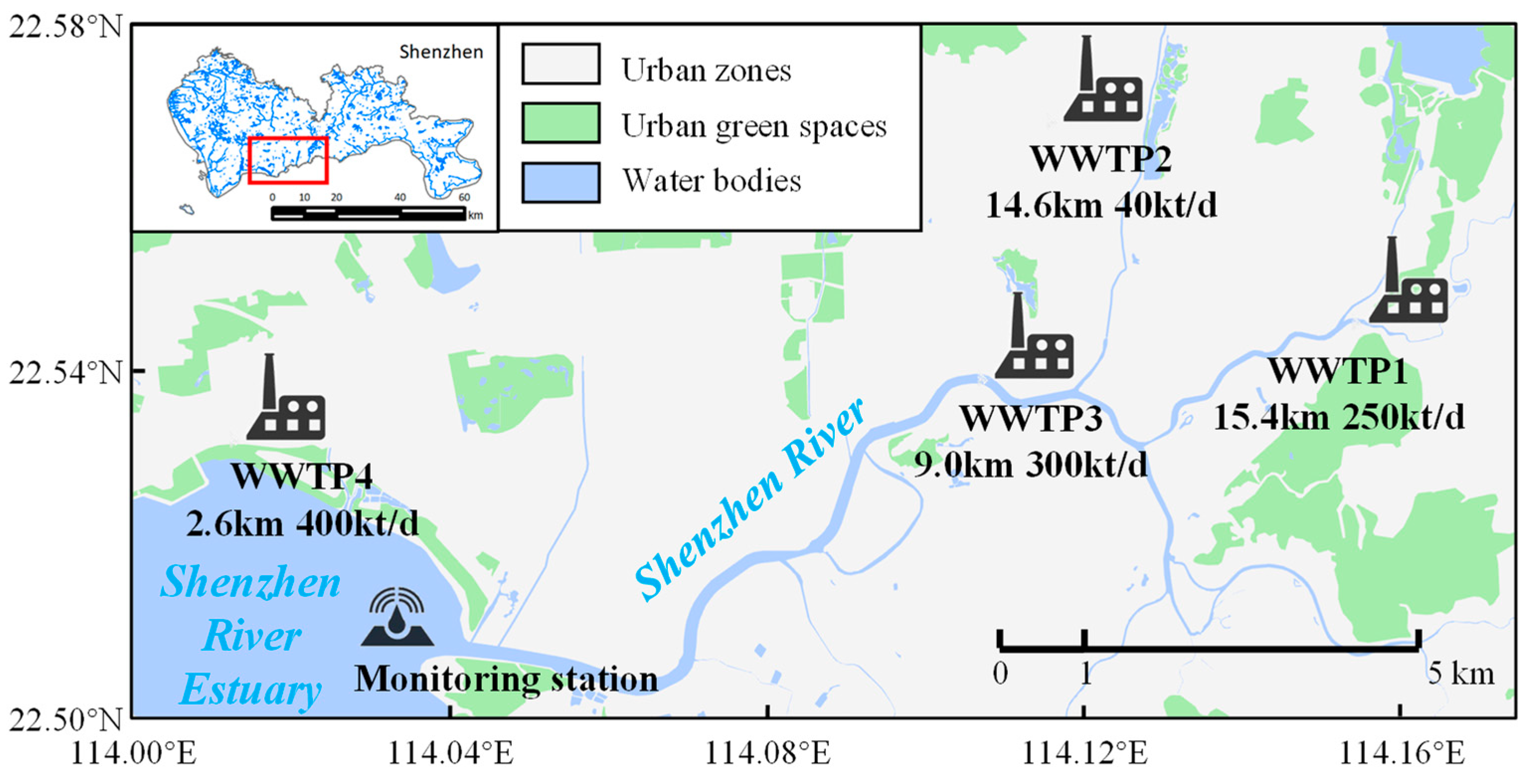
2.1. Study Area

This investigation focuses on the hypoxia phenomenon in the Shenzhen River Estuary (SRE), located in Shenzhen in southern China. Four WWTPs are located in the Shenzhen River watershed. A map of their locations, distances to the monitoring station in the SRE, and their daily treatment capacities are shown in Figure 1: gray-shaded areas represent urban zones, green areas denote urban green spaces, and blue regions depict water bodies. Characterized by intensive anthropogenic activities and complex hydrodynamic conditions, this estuary exhibits persistent seasonal hypoxia, making it a representative system for studying low DO driving factors in subtropical estuaries.

Water quality monitoring datasets spanning 2022–2023 were analyzed, encompassing more than 20 parameters collected through in situ measurements and automated sensor networks deployed at the SRE. Four critical parameters were selected for driver analysis: (1) dissolved oxygen (DO), (2) temperature, (3) Turbidity, and (4) total nitrogen (TN). These variables were prioritized based on their established correlations with hypoxia mechanisms in comparable estuarine systems. The monitoring data range from January to August 2022 and January to August 2023.

Datasets of the four WWTPs’ daily treatment capacity and three parameters of outlet water—(1) biochemical carbon demand (BOD), (2) suspended solids (SSs), and (3) total nitrogen (TN)—with the same time range as the monitoring data, are also included in this study. These data were obtained through the monitoring equipment set at the WWTP outlets.

Detailed information of the datasets, including sources, parameter types, and time solutions, is listed in

Table 1. Detailed information of the datasets from the SRE and WWTP outlets.

Data Source	Parameter	Time Resolution
SRE monitoring station	Temperature	Every hour (after 10 May 2022); Every 4 h (before 29 April 2022)
	DO
	Turbidity
	TN	Every 4 h
WWTP outlet monitoring stations	WWTP treatment capacity	Daily
	BOD
	SS
	TN

.

The raw datasets were preprocessed to ensure data quality prior to analysis. Based on the time resolution of the in situ sensing equipment, duplicate entries and erroneous values were systematically removed. Missing data points were then reconstructed using linear interpolation to maintain temporal continuity. Following preprocessing, comparative boxplots were generated to analyze the structural variations in the water quality parameters between the 2022 and 2023 SRE monitoring datasets (Figure 2).

It is shown that the median DO level increased from 3.5 mg/L in 2022 to 4.8 mg/L in 2023, indicating a significant improvement in oxygen saturation. The temperature in 2022 was generally higher than that in 2023, and the distribution of high temperature data was denser than in 2023. For Turbidity, minimal interannual differences were observed, suggesting stable SS levels. Higher TN concentrations in 2023 than in 2022 imply intensified nutrient pollution, potentially linked to anthropogenic activities or seasonal runoff variations.

2.2. Anomaly Detection Method Based on Wavelet Analysis and the Temporal Entropy Index

Accurate detection of hypoxia events requires both the qualitative identification of spatiotemporal patterns and the quantitative assessment of severity. Given that conventional single-method approaches often fail to comprehensively address these dual dimensions, this study employs complementary methodologies: continuous wavelet transform (CWT) for the qualitative characterization of event timing and anomaly signatures and information entropy (IE) for the quantitative evaluation of hypoxia intensity. This integrated framework balances visual interpretability with rigorous statistical measurements.

2.2.1. Wavelet Analysis

Wavelet analysis is a powerful tool for detecting anomalies in time-series data, particularly in water quality monitoring, where data often exhibit non-stationary and multi-scale characteristics. Unlike traditional Fourier transforms, wavelet transforms provide both time and frequency localization, making them highly effective for identifying transient anomalies and trends at different temporal scales.

The continuous wavelet transform (CWT) is commonly used for anomaly detection. Given a time-series signal x(t), the CWT is defined as follows:

$$W\left(a,b\right)={\displaystyle \frac{1}{\sqrt{a}}}{\displaystyle {\int }_{-\infty }^{\infty }x\left(t\right)\psi *\left(\frac{t-b}{a}\right)\mathrm{d}t}$$

(1)

where a is the scale parameter, b is the translation parameter, and ψ(t) is the mother wavelet function. The Morlet wavelet, defined as $\psi \left(t\right)={\pi }^{-1/4}{e}^{i{\omega }_{0}t}{e}^{-t^2/2}$, is often used due to its balance between time and frequency resolution.

In water quality monitoring, anomalies such as sudden drops in DO or spikes in Turbidity can be detected by analyzing the wavelet coefficients W(a,b). Significant deviations in the wavelet power spectrum, calculated as |W(a,b)|², indicate potential anomalies. Additionally, the wavelet transform can decompose the signal into different frequency bands, allowing for the identification of anomalies at specific scales, such as diurnal or seasonal variations.

To enhance detection accuracy, a thresholding method is often applied to wavelet coefficients. For example, a universal threshold $\lambda =\sigma \sqrt{2\ln N}$ can be used, where σ is the noise standard deviation and N is the number of data points. Coefficients exceeding this threshold are flagged as anomalies.

Wavelet analysis has been successfully applied in various water quality studies, demonstrating its robustness in detecting anomalies and trends in complex environmental datasets [27,28].

According to Jiang, et al. [29], two distinct anomaly patterns can be detected via CWT. Type I anomalies, characterized by abrupt short-term shifts in DO concentrations (e.g., sudden rises or declines), manifest as localized spectral peaks (high-intensity regions) on the CWT scalogram. The magnitude of these shifts is semi-quantitatively reflected by the color intensity of the peaks. Type II anomalies, defined by amplified temporal swings in DO values, appear as enhanced low-frequency contours (bright-colored bands) on the scalogram, indicating prolonged periods of increased hydrodynamic or metabolic variability.

2.2.2. Temporal Entropy Index

Information entropy quantifies system uncertainty and complexity, forming the theoretical foundation for the temporal entropy index (G_t). Applied to water quality time-series data, G_t measures temporal uncertainty and, when integrated with wavelet analysis and Fourier transform, identifies structural heterogeneity, periodicity, and anomalous pollution events in high-frequency datasets. By establishing predefined thresholds, deviations in G_t values can trigger alerts for abnormal events, offering a systematic approach to anomaly detection.

The temporal dynamics of G_t further enable differentiation between distinct time-series patterns (e.g., random vs. chaotic sequences) and evaluation of data predictability. This methodology proves particularly effective for discerning structural variations in water quality under diverse hydrological conditions and pinpointing critical transition points in temporal patterns.

G_t outperforms traditional methods in complex environmental systems by capturing nuanced behavioral shifts in water quality parameters. Its synergy with multi-scale analytical techniques enhances sensitivity to subtle system anomalies, positioning it as a powerful tool for environmental monitoring and adaptive management.

In this study, G_t is computed as a binary cross-entropy [30] using DO monitoring data within a defined temporal window (termed a “cell”, e.g., a 12 h interval). Data within the cell are classified into two groups based on a concentration threshold C_t (higher than the threshold and lower than the threshold). Values exceeding C_t (N_h) and values falling below C_t (N_l) and the frequency p_h and p_l of the two groups of data are calculated as below:

$$p_h={\displaystyle \frac{N_h}{N_h+N_l}},p_l={\displaystyle \frac{N_l}{N_h+N_l}}$$

(2)

The temporal entropy index G_t is calculated with p_h and p_l according to the definition of G_t:

$$G_t=p_h\ln p_h+p_l\ln p_l$$

(3)

A decision variable R_w, representing the temporal rate of change of G_t, is defined as follows:

$$R_w={\displaystyle \frac{\Delta G_t}{\Delta t}}$$

(4)

Operational responses to anomaly detection are guided by R_w:

• Baseline condition: If all DO values within the cell remain below C_t, G_t and R_w equal 0, indicating normal water quality;
• Warning phase: R_w > 0 signals threshold exceedance, triggering an anomaly alert;
• Critical action: Sustained R_w > 0 over consecutive intervals confirms an anomaly;
• Recovery: When R_w ≤ 0 and DO values stabilize below C_t, normal operations resume.

This framework enables real-time risk assessment and adaptive water management, balancing sensitivity to anomalies with robustness against false alarms.

2.3. Driving Factor Analysis Method Based on Pearson Correlation Coefficients and Transfer Entropy

2.3.1. Pearson Correlation Coefficients

The temporal dynamics of DO were investigated through correlation analysis with key water quality parameters (water temperature, Turbidity, and TN) using Pearson correlation coefficients and linear regression models. Scatter plots with fitted curves were generated to visualize relationships.

The Pearson correlation coefficient (PCC) is a statistical tool that measures linear correlation between two sets of data. The coefficient represents the ratio between the covariance of two variables and the product of their standard deviations. In this study, PCC was employed to quantify linear relationships between DO and physicochemical parameters (e.g., water temperature, Turbidity). PCC values range from −1 (perfect negative correlation) to +1 (perfect positive correlation), calculated as follows:

$$r={\displaystyle \frac{{\displaystyle \sum \left(X_i-\overline{X}\right)\left(Y_i-\overline{Y}\right)}}{\sqrt{{\displaystyle \sum {\left(X_i-\overline{X}\right)}^2}{\displaystyle \sum {\left(Y_i-\overline{Y}\right)}^2}}}}$$

(5)

where X and Y are two variables, and $\overline{X}$ and $\overline{Y}$ are the mean of the sample. Significance of the correlations was assessed via two-tailed t-tests (α = 0.05). Linear regression models further characterized the direction and magnitude of relationships, with goodness of fit evaluated by R².

Moreover, to account for diurnal variations driven by organic degradation and biological respiration (notably, the absence of photosynthesis at night), DO data were categorized into “Dark” (02:00–05:00) and “Daylight” (all other hours) [31]. Kernel density distribution (KDE) plots were employed to contrast the diurnal patterns of DO, water temperature, Turbidity, and total nitrogen. Separate correlation analyses were conducted for Dark subsets to identify distinct drivers of hypoxic conditions in the SRE. KDE is a non-parametric statistical method used to estimate the probability density function (PDF) of a continuous random variable. Unlike histograms, which bin data into discrete intervals, KDE smooths observations using a kernel function, providing a continuous and differentiable density curve. This technique is particularly useful for visualizing the underlying distribution of data and comparing subpopulations. The estimated density $\widehat{f}\left(x\right)$ at a point $x$ is calculated as follows:

$$\widehat{f}\left(x\right)={\displaystyle \frac{1}{nh}}{\displaystyle \sum _{i=1}^{n}K\left(\frac{x-X_i}{h}\right)}$$

(6)

where X_i represents the observed data points, K(·) is the kernel function, and h defines the bandwidth that controls the trade-off between bias and variance.

2.3.2. Transfer Entropy

Transfer entropy (TE), introduced by Schreiber [32] in 2000, is an information-theoretic measure to quantify directed (time-asymmetric) information flow between dynamical systems. It evaluates how much the uncertainty of a future state of a target variable Y is reduced by incorporating the past of a source variable X beyond the information already contained in the past of Y. The discrete TE is formally defined as follows:

$$T_{X\to Y}=H\left(Y_t|Y_{t-1}\right)-H\left(Y_t|Y_{t-1},X_{t-1}\right)$$

(7)

where H(·|·) refers to conditional Shannon entropy:

$$H\left(Y_t|Y_{t-1}\right)=H\left(Y_t,Y_{t-1}\right)-H\left(Y_{t-1}\right)$$

(8)

The calculation steps of TE can be found in the Supplementary Information.

For the two variables X and Y, if T_X→Y > T_Y→X, it suggests that X has a causal relationship with Y.

TE offers a robust, assumption-free approach to unravel causal interactions in complex environmental systems, which is one of the information-theoretic approaches widely adopted in water environment and resource management. Bharti, et al. [33] used TE to analyze causal relationships in the complex network of groundwater levels. Zhu, et al. [34] proposed an R-vine Copula TE method for high-dimensional causal analysis in ecological networks, applicable to pollutant transport modeling in river basins.

3. Results

3.1. Anomaly Detection in the Hypoxia Phenomenon

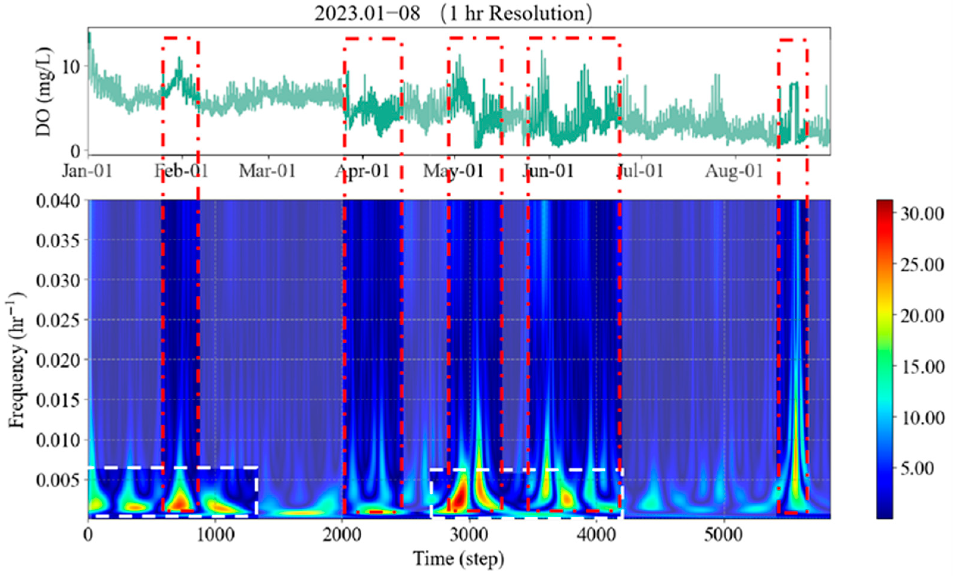
3.1.1. Hypoxia Event Identification by CWT

Continuous wavelet transform (CWT) was employed to identify anomalies in DO time series through frequency–domain analysis. The DO time series exhibited pronounced diurnal periodicity, with regular daytime increases and nighttime declines. Notably, Type I and Type II anomalies frequently co-occurred; abrupt DO shifts (Type I) were often accompanied by intensified low-frequency oscillations (Type II), suggesting synergistic interactions between instantaneous disturbances and sustained environmental perturbations.

As shown in Figure 3, at the beginning of the year 2023, a significant DO decline coincided with heightened oscillations, evidenced by prominent scalogram peaks and bright low-frequency bands. Moderate DO increases in mid-January and early February can also be seen, with detectable Type I/II anomalies. From February to early March, DO fluctuations remained relatively subdued, except for a moderate oscillation surge in mid-February, reflected by faint spectral peaks and limited bright contours. During April, two distinct DO abrupt shifts were observed, aligned with transient spectral peaks and diffuse low-frequency signals. By May, DO variability intensified markedly, with severe fluctuations, including a significant decline at the beginning of the month. May saw the most abrupt DO shift of the year, reflected in the CWT results by sustained bright low-frequency bands, indicating prolonged hydrodynamic instability. Fluctuations continued in June, and July was a relatively normal month. In August, an abrupt change was detected, with few low-frequency oscillations observed.

CWT demonstrates strong capabilities in identifying abrupt changes and unstable fluctuations in DO time series [35]. By analyzing frequency–domain signatures, CWT effectively localizes anomalous DO segments and visually represents these anomalies through scalogram visualizations (e.g., spectral peaks and low-frequency contours), enabling intuitive interpretation of transient disturbances. However, CWT still has limitations in practical applications. For Type I anomalies (sudden DO shifts), while CWT can pinpoint the temporal occurrence of abrupt changes, it fails to identify the shift direction (e.g., rising vs. declining trends) and lacks the capability for quantitative assessment of the magnitude of deviations. This poses challenges in scenarios requiring threshold-based alerts, such as detecting sudden DO declines caused by abrupt contamination events. Specifically, CWT cannot directly evaluate whether DO concentrations fall below critical thresholds (e.g., water quality standards) or trigger warnings based on predefined risk levels, limiting its utility in real-time pollution monitoring systems.

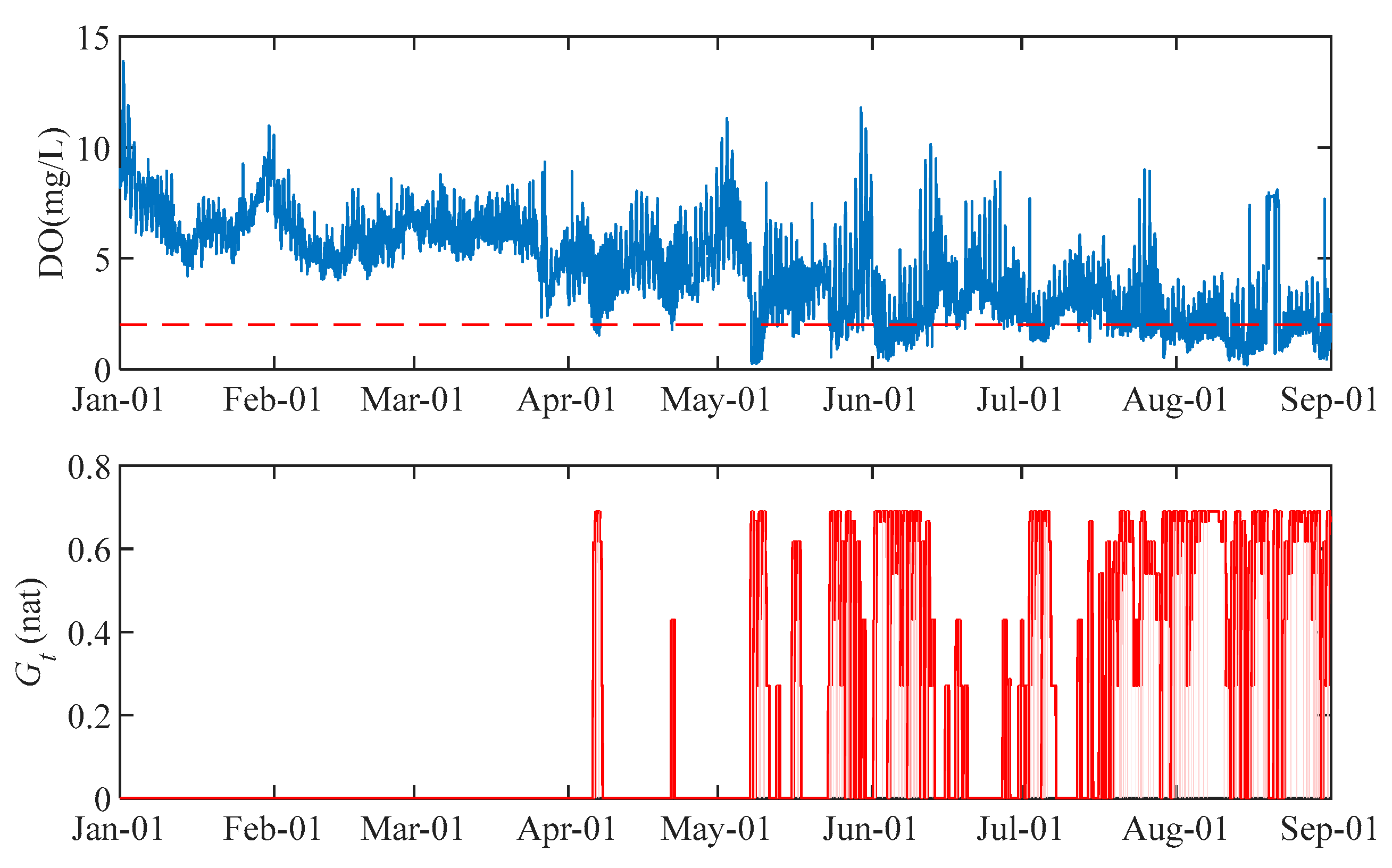
3.1.2. Hypoxia Event Identification by Temporal Information Entropy

DO data from the estuary from January to May 2023 were chosen for anomaly detection. When calculating the time entropy index G_t, two parameters, time cell length = 12 h and DO threshold C_t = 2 mg/L, were selected.

The results of the temporal entropy index are presented in Figure 4. As shown, the anomaly detection algorithm based on the temporal entropy index successfully identified hypoxia events occurring from April to August, and the frequency and duration of hypoxia events in summer (June–August) were significantly higher and longer than those in winter and spring (January–May). This method successfully detected the hypoxia events in July and August that could not be identified by the CWT method, where DO concentrations are lower than the threshold. In February, considered by CWT to have an anomaly, the temporal entropy index remained at zero despite minor fluctuations in DO values, indicating no hypoxia event. However, once a single monitoring datum fell below the threshold (red line in the DO curve), the algorithm promptly detected the anomaly and generated a distinct entropy peak, demonstrating its high sensitivity.

Furthermore, when transient DO measurements briefly rebounded above the threshold before dropping below it again, the temporal entropy index effectively smoothed out such fluctuations by consolidating consecutive sub-threshold DO troughs into a unified entropy peak. This capability highlights the algorithm’s robustness in mitigating the impact of sporadic data noise, thereby enhancing detection stability.

In comparison to wavelet analysis, the temporal entropy index-based anomaly detection algorithm operates under predefined event thresholds, achieving a balance between sensitivity and robustness. However, its utility is inherently constrained when the monitoring data persistently remain above the threshold, as the method cannot be activated under such conditions.

3.2. Analysis of Driving Factors of Hypoxia Events

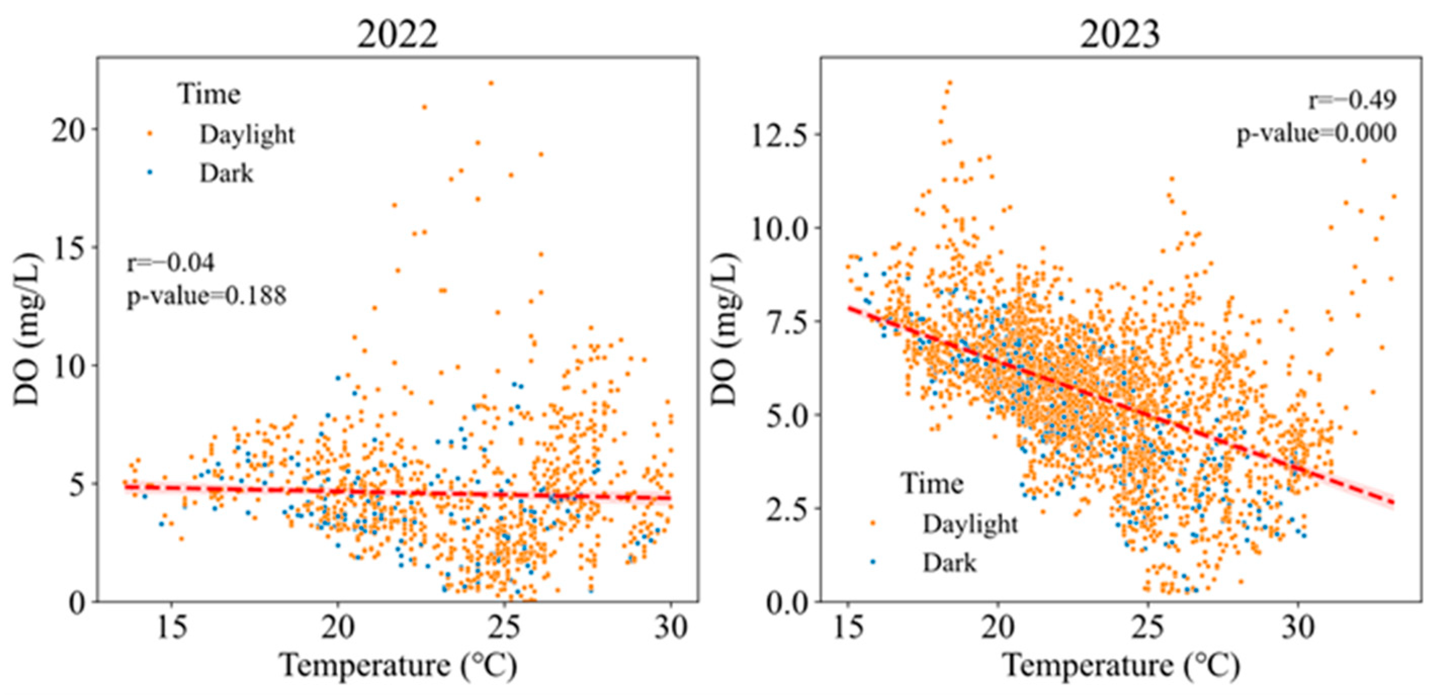
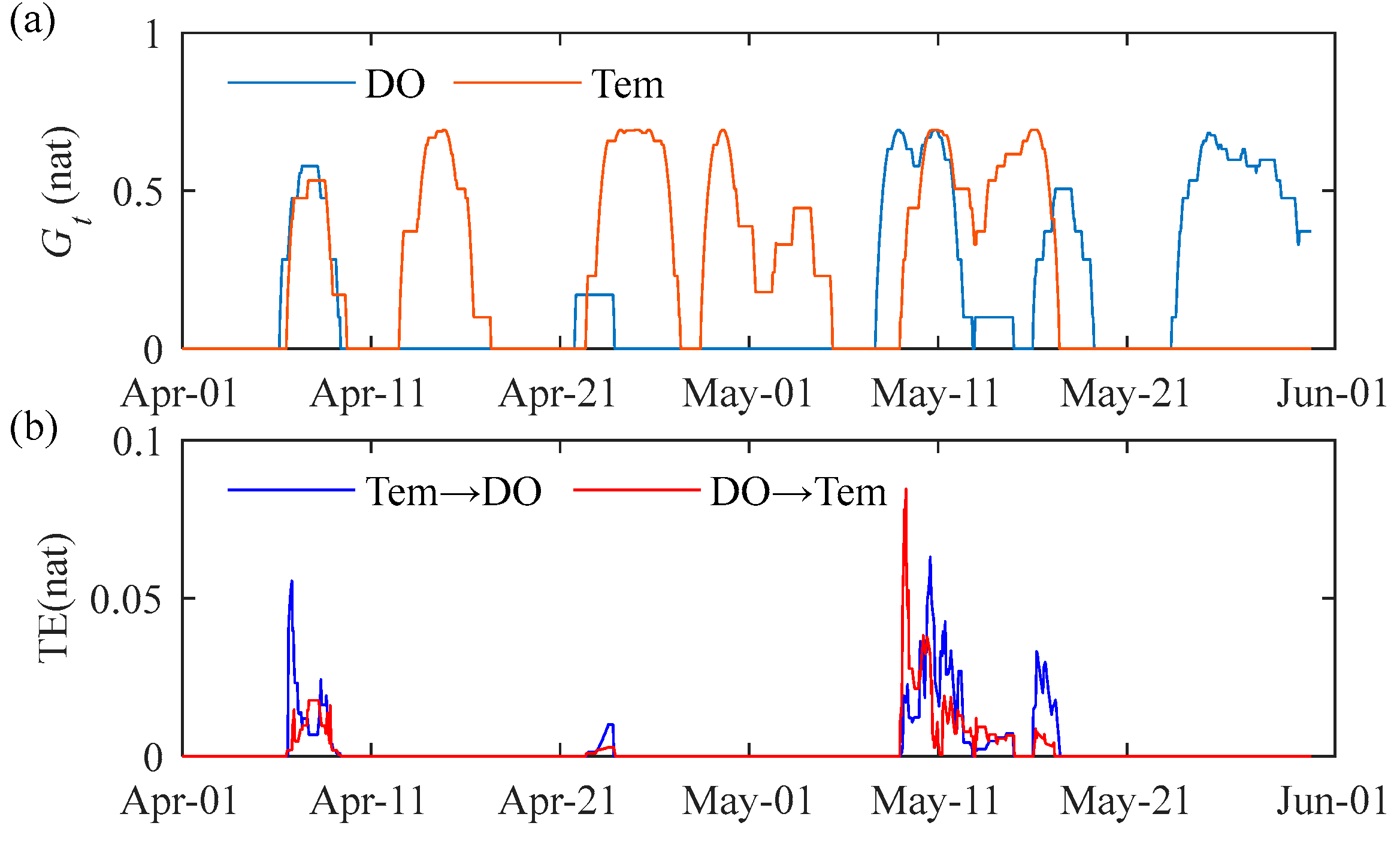
3.2.1. Water Temperature

On a daily scale, the driving effect of temperature on hypoxic events is manifested in the difference in temperature between day and night. Figure 5 shows the distribution of DO values during dark (from 02:00 to 05:00) and daylight (the remainder) hours. DO levels consistently decreased during the dark period, attributable to the absence of photosynthesis, lower temperatures, and heightened oxygen demand by aquatic organisms. The phenological cycle of aquatic vegetation and metabolic activities of microorganisms such as cyanobacteria (blue–green algae) likely contribute to this DO pattern. Photosynthetic oxygen production by aquatic plants exhibits fluctuations, while cyanobacterial blooms during warmer periods create dual oxygen dynamics through daytime photosynthesis and nighttime respiration, potentially intensifying oxygen depletion. Notably, diurnal fluctuations in DO were significant due to biological and physicochemical processes. During daylight periods, photosynthetic activity contributes to oxygen production, whereas dark periods rely solely on surface reaeration, compounded by oxygen consumption from organic degradation and respiration.

While temperature inversely affects saturated DO levels, its role in driving extreme hypoxic events was limited. In 2022, temperature exhibited no significant correlation with DO (r = −0.04, p = 0.188). In 2023, a stronger negative correlation emerged (r = −0.49, p < 0.001), suggesting the temperature-mediated suppression of DO (Figure 6). However, calculated theoretical saturated DO values for observed temperatures revealed that measured DO levels were substantially lower than predicted in both years, implying that temperature alone cannot explain extreme DO depletion, necessitating investigation of additional drivers.

Furthermore, analysis of the DO time series revealed distinct seasonal patterns. Higher DO levels were observed in early months of the year, followed by a gradual decline. In 2022, nearly half of the first half-year exhibited DO concentrations below 5 mg/L in the SRE, while conditions improved slightly in 2023. However, both years showed a marked increase in non-compliant DO episodes (concentrations falling below regulatory thresholds) after April, with extreme events reaching levels below 2 mg/L. This seasonal pattern may be primarily attributed to thermal variations across seasons. Elevated water temperatures typically reduce oxygen solubility, theoretically lowering saturated DO levels and thereby exacerbating hypoxic conditions during spring and summer months.

In response to hypoxia events occurring in April and May 2023, G_t was utilized to determine whether anomalies were present in the temperature and DO values. Additionally, TE between the DO data and temperature was calculated. A temperature threshold of 25 °C was applied during the computation process.

The results are presented in Figure 7. It can be observed that during the hypoxia event around 7 April, temperature anomalies were also detected. The TE results between the two indicate a significant correlation between this DO anomaly event and the abnormal rise in temperature. However, for the hypoxia events on 22 April and 7 May, although temperature anomalies were also detected, there was a temporal lag. Furthermore, during the hypoxia event on May 23rd, no temperature anomalies were detected. This suggests that while elevated temperatures may contribute to hypoxia in some cases, they are not the definitive driving factor for such events.

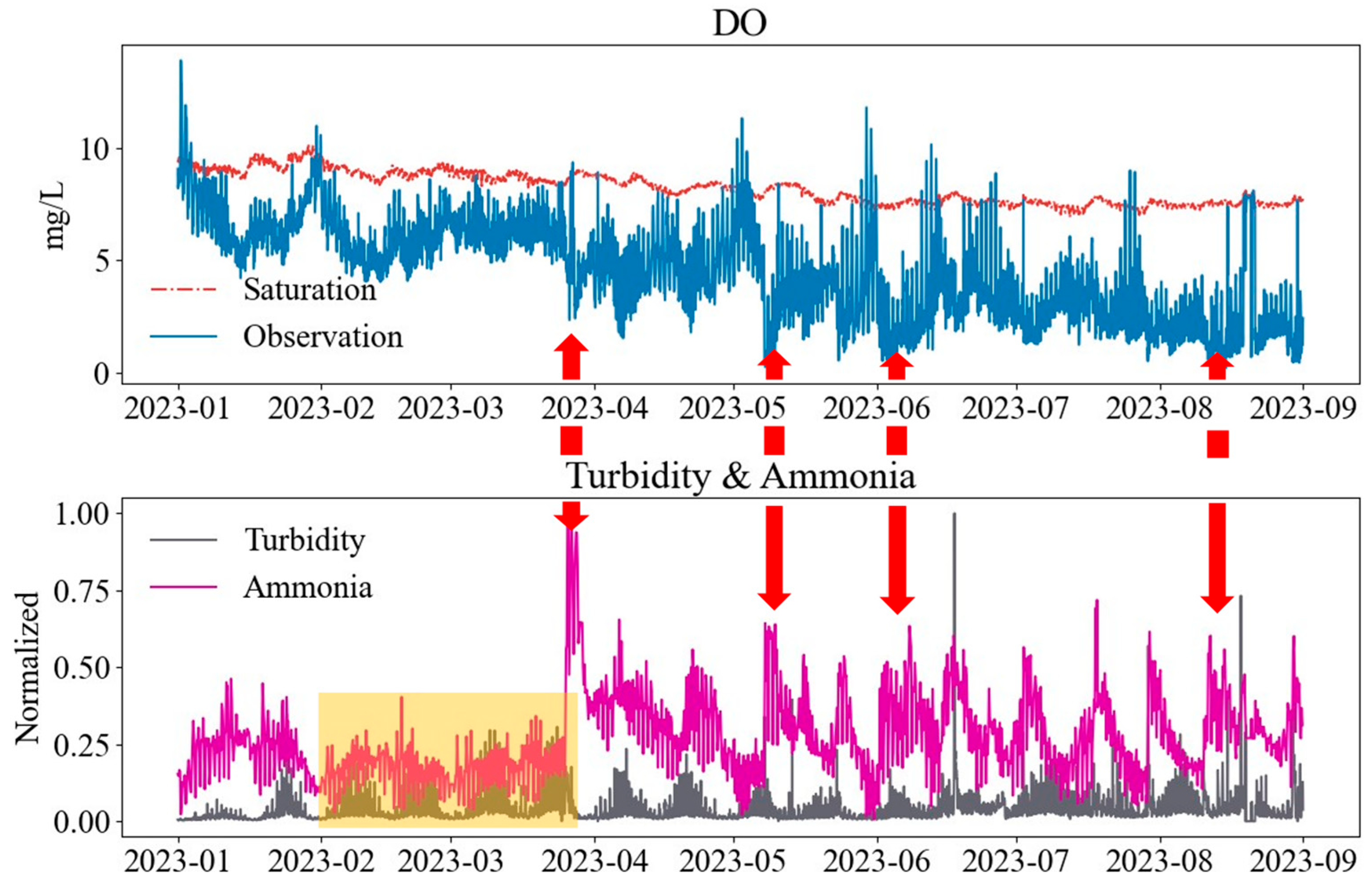
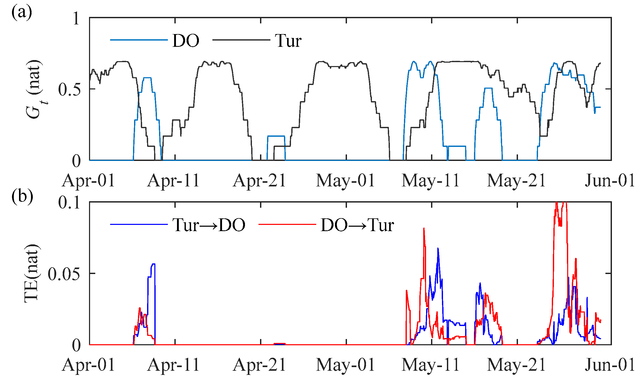
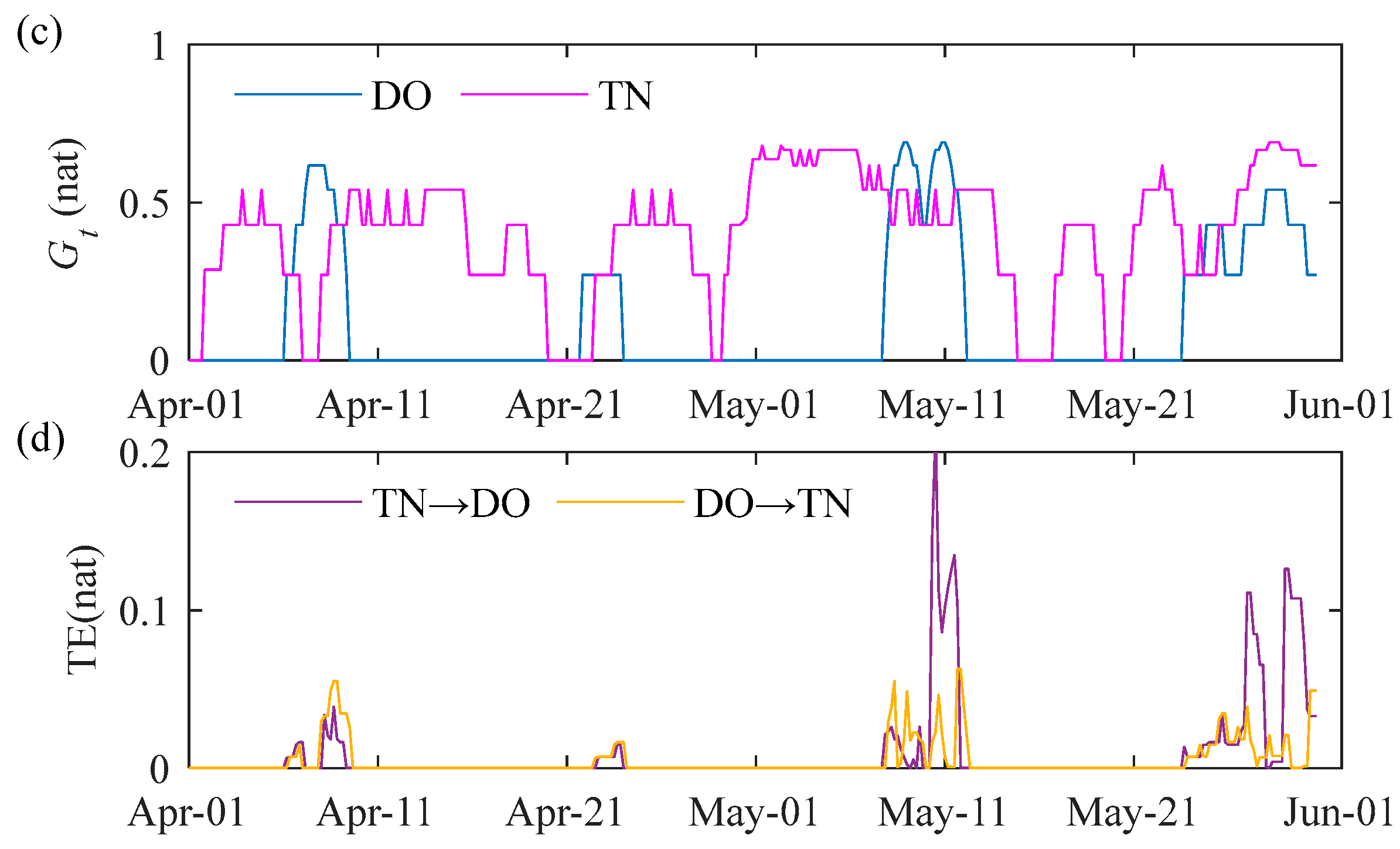
3.2.2. Turbidity, Ammonia, and Total Nitrogen

Turbidity demonstrated significant negative correlations with DO in both years (2022: r = −0.29; 2023: r = −0.15; p < 0.01 for both). Time-series alignment identified Turbidity peaks coinciding with abrupt DO declines, indicating that sediment-laden inflows may directly exacerbate hypoxia. Turbidity also displayed periodic patterns, with bimonthly peaks and daily cycles. Elevated Turbidity occurred predominantly during the hours of 07:00–12:00 and 19:00–00:00, aligning with anthropogenic water usage peaks. This synchronicity suggests potential linkage to wastewater discharges from upstream treatment plants. Although rainfall is a common Turbidity driver, meteorological records ruled out precipitation as a contributor to the 2023 Turbidity periodicity, reinforcing the hypothesis of anthropogenic origins.

Ammonia nitrogen (NH₃-N) and total nitrogen (TN) exhibited strong negative correlations with DO (2022 NH₃-N: r = −0.33; 2023 NH₃-N: r = −0.66; 2022 TN: r = −0.11; 2023 TN: r = −0.40; p < 0.01 for all). NH₃-N concentrations displayed seasonal peaks in May 2022 and April 2023, with diurnal patterns mirroring Turbidity trends (Figure 8), implying shared pollution sources. In 2023, NH₃-N exceedances (>1.0 mg/L) surged from 23 episodes in January (primarily at 12:00 and 16:00) to 61 episodes in May, with new nighttime peaks emerging at 00:00 and 04:00. Concurrently, TN violations were more frequent and evenly distributed across daytime hours. Elevated nighttime NH₃-N and TN levels in May—the month with the lowest average DO—suggest intensified ammonification of organic nitrogen under hypoxic conditions. This process releases CO₂, acidifying the water (lowering pH) and further inhibiting nitrification, thereby perpetuating oxygen depletion. The significant positive correlation between pH and DO (2022: r = 0.55; 2023: r = 0.69) supports this mechanism, as pH dynamics are tightly coupled to nitrogen transformation pathways.

Transfer entropy (TE) is utilized to analyze the driving effects of Turbidity and TN on DO values. Figure 9 shows the results of anomaly detection in Turbidity and TN values based on G_t, as well as the calculated TE between the DO data and Turbidity/TN. During the computation, the threshold for Turbidity was set at 40 NTU, with 4 mg/L for TN.

The results indicate that during the three hypoxia events, TE from DO to Turbidity was greater than that from Turbidity to DO in the initial stages. This suggests that the initial DO anomalies led to Turbidity anomalies, which aligns with the G_t criterion showing that the peak in Turbidity anomalies lagged behind that in DO anomalies. As time progressed, TE from Turbidity to DO surpassed that from DO to Turbidity, indicating that Turbidity anomalies subsequently caused DO anomalies. This is because high Turbidity reduces water transparency, affecting algal photosynthesis, which is primarily a reaeration process. Additionally, Turbidity is primarily derived from degradable organic matter, whose decomposition consumes DO. The combined effects of these factors contribute to the occurrence of hypoxia events.

For TN, during the initial stages of the hypoxia events, the TE between TN and DO was nearly equal, indicating a mutual influence. This is due to the diverse types of pollutants associated with TN, including oxygen-consuming nitrification and anaerobic denitrification processes. As a result, the influence between TN and DO is bidirectional. However, in the middle and later stages of the events, TE from TN to DO began to exceed that from DO to TN, indicating that TN started to dominate in the hypoxia events.

To validate the lag effect of pollutants on the driving of hypoxia events, the pollutant concentration data from several hours before the hypoxia event in April 2023 were selected, and TE was used to determine the time-lag influence. The results are shown in Figure 10.

The results indicate that the time lag of pollutant loads on DO varies across different stages of the same hypoxia event. For Turbidity, the highest transfer entropy and strongest influence during the early stage of the hypoxia event were observed for loads from 36 h earlier. During the middle stage, the highest transfer entropy shifted to loads from 48 h earlier, while in the late stage, it was associated with loads from 12 h earlier. For hypoxia event forecasting, greater attention should be paid to pollutant load information, which has a more significant impact during the early stage, especially Turbidity data from 36 h earlier. In contrast, for TN, the highest transfer entropy in most periods was observed for loads from 72 h earlier, indicating that the time lag in TN’s influence on DO is approximately 72 h.

TE can quantitatively describe the driving force of water quality parameter disturbances on DO changes. Although the peak TE values of Turbidity and TN on DO during hypoxia events were comparable (around 0.05 nat), the discharge of suspended solid (SS) pollution is often greater, causing Turbidity to be a stronger driving force. Therefore, it can be concluded that the driving force of Turbidity on low DO events is greater than that of TN.

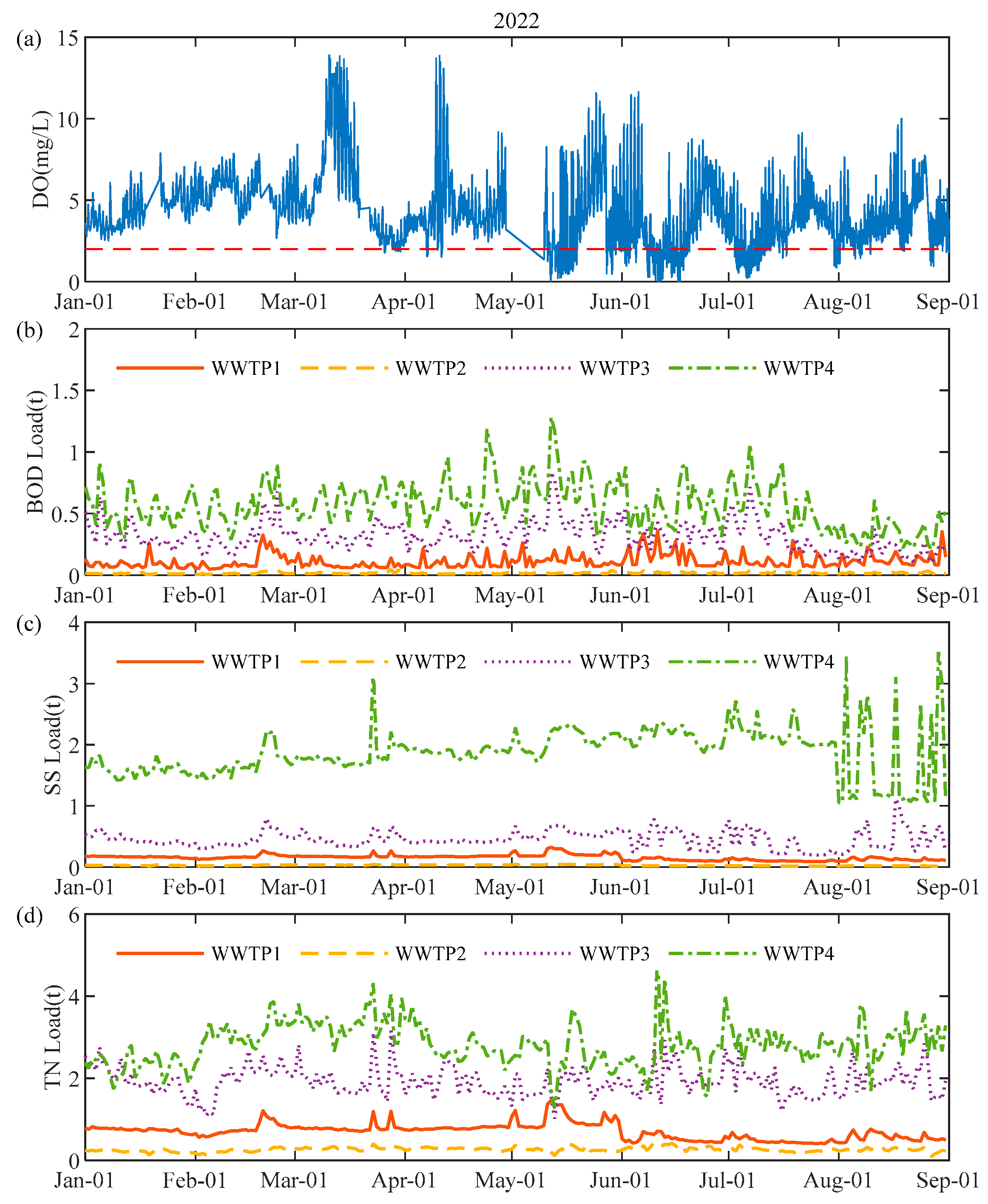
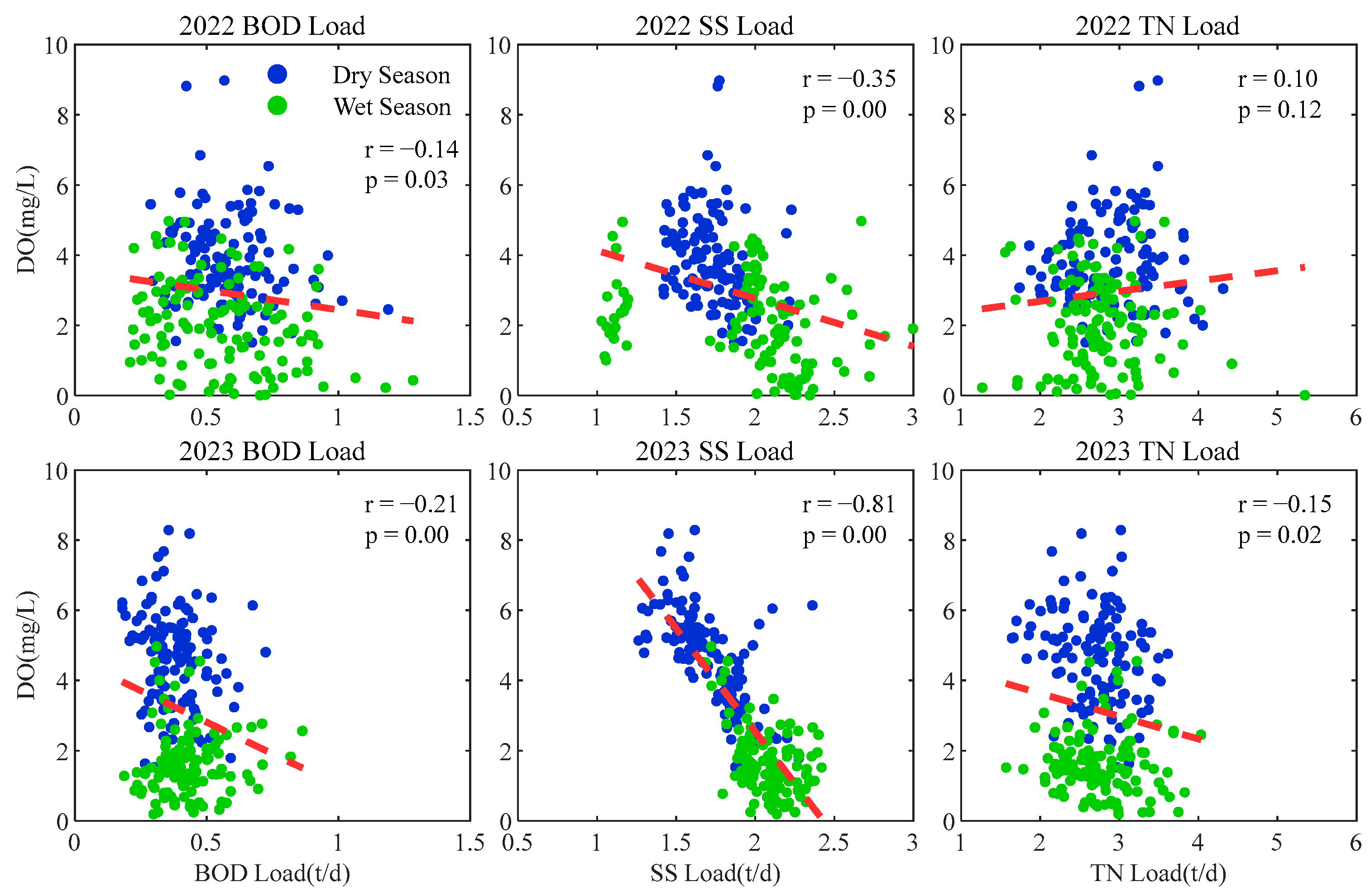
3.2.3. Correlation Analysis Between Hypoxia Events and WWTP Pollution Loads

Due to the attenuation of pollutant loads discharged from different upstream locations in the river during their migration, preprocessing is necessary to compare the contributions of pollutant loads from different wastewater treatment plants (WWTPs) on a unified basis. This involves converting the pollutant loads from all WWTPs into equivalent pollutant loads at monitoring stations to account for degradation and attenuation effects during pollutant transport. Due to WWTP4 being next to the SRE, we only converted the loads of the other three WWTPs upstream of the Shenzhen River.

In this study, the daily pollutant loads from WWTPs were processed using the first-order reaction kinetics formula:

$$L_{ij}=Q_i{C}_{ij}=Q_i{C}_{ij,0}{e}^{-k_j{x}_i/u.}$$

(9)

where L_ij is the daily load of jth pollutant from ith WWTP, Q_i is the daily discharge of ith WWTP, C_ij is the concentration of jth load at ith WWTP, C_ij,0 is the original concentration, k_j is the degradation coefficient of jth load, x_i is the distance from ith WWTP to the monitoring station in SRE, and u is the velocity of river flow.

The coefficients used are listed in

Table 2. Coefficients used in WWTP load preprocessing.

Coefficient	Explanation	Value
k1	Degradation coefficient of BOD (d−1)	0.25
k2	Degradation coefficient of SS (d−1)	1
k3	Degradation coefficient of TN (d−1)	0.15
x1	Distance from WWTP1 to the estuary (km)	15.4
x2	Distance from WWTP2 to the estuary (km)	14.6
x3	Distance from WWTP3 to the estuary (km)	9
u	Velocity of river flow (km/d)	8.64

.

The trends in DO changes in the estuary from January to August 2022 and January to August 2023, along with the equivalent daily pollutant loads of BOD, SS, and TN discharged from the four WWTPs during the corresponding periods, are shown in Figure 11.

The results indicate that the pollutant load contribution from WWTP4 is significantly greater than that from the other three WWTPs. This conclusion is evident because WWTP4 is the closest to the estuary and has the largest average daily wastewater treatment volume. Given that the effluent quality indicators are similar, its pollutant load contribution should logically be the highest.

A Pearson correlation test was conducted between the daily loads from WWTP4, which has the largest contribution, and the corresponding daily minimum DO values at the estuary. Data are divided into two sets: the dry season (January–April) and the wet season (May–August). The results are shown in Figure 12. The 2023 data show that BOD, SSs, and TN all exhibit negative correlations with DO levels, with SSs showing the strongest linear correlation (r = −0.81), followed by BOD, and TN is the weakest. This result can be explained from physical and chemical perspectives—high concentrations of SSs can hinder water transparency, inhibiting algal photosynthesis (a primary source of DO). Additionally, SSs often serve as a carrier for organic pollutants and nutrients, and the settling of particles can cover sediments, potentially exacerbating anaerobic reactions at the bottom and releasing reducing substances that indirectly consume DO. BOD, representing organic matter, requires gradual microbial decomposition, and the oxygen consumption process exhibits a time lag (e.g., the disconnect between BOD and instantaneous DO). Moreover, BOD includes refractory organic matter (e.g., lignin), which has a low oxygen consumption contribution, possibly diluting the overall correlation strength. TN includes various forms such as organic nitrogen and ammonia nitrogen, and different forms have varying effects on DO. For instance, denitrification processes can partially offset net oxygen consumption, reducing statistical significance.

The figure further reveals that daily minimum dissolved oxygen (DO) concentrations during the dry season are consistently higher than those in the wet season, aligning with previous conclusions that hypoxia events predominantly occur in spring and summer. In 2022, pollutant load data generally showed no correlation with DO except for SSs, consistent with the earlier observation that temperature and DO were also uncorrelated in 2022. This is likely due to the high baseline influence in 2022. After one year of remediation efforts, the water quality of the Shenzhen River improved significantly, making the impact of WWTP discharges on estuarine DO more pronounced in 2023.

4. Discussion

4.1. Comparison and Combination of Anomaly Detection Methods

Wavelet anomaly detection can decompose signals at different scales, capturing both long-term trends (low-frequency components) and sudden pollution events (high-frequency mutations) in dissolved oxygen (DO) sequences. It also adapts better to non-stationary signals compared to Fourier transform, making it particularly suitable for detecting pulse-type anomalies (e.g., instantaneous exceedances at discharge outlets) commonly found in water environment data. However, it cannot directly associate specific water quality thresholds (e.g., hypoxia events where DO < 2 mg/L) and lacks an adaptive mechanism.

In contrast, the entropy index method quantifies the degree of deviation of a sequence from a preset threshold based on the statistical characteristics of the original sequence. It is particularly suitable for detecting anomaly events requiring rapid responses from real-time monitoring systems, such as DO levels falling below ecological thresholds. Additionally, it is insensitive to sporadic anomalies, such as single-point data anomalies caused by occasional instrument malfunctions, which do not significantly alter the overall entropy value, thereby reducing false alarm rates. However, when DO levels are generally above the threshold but experience instantaneous sharp declines, entropy changes may be smoothed out and obscured. Moreover, it cannot distinguish between normal fluctuations near the threshold and true anomalies, nor can it pinpoint the exact timing of anomalies as precisely as wavelet analysis.

Therefore, the two anomaly detection methods can be combined. In the first layer, discrete wavelet transform is used to extract high-frequency detail components of the DO sequence, detecting sudden anomalies (e.g., instantaneous oxygen consumption caused by BOD shock loads) and marking their time locations. In the second layer, sliding window entropy is calculated for the low-frequency approximation components to identify persistent hypoxia events (e.g., long-term hypoxia induced by TN accumulation). By combining threshold-based judgments of ecological risk levels, a complementary paradigm of “high-frequency localization and low-frequency assessment” can be established, achieving complementary strengths, enhancing the sensitivity and robustness of anomaly event detection. In the future, this approach can be further enhanced by integrating machine learning and physical models (e.g., water quality kinetic equations) to improve parameter adaptability and mechanistic interpretability.

4.2. Driving Factors of Hypoxia Events and the Lag Effect of Factors

Through data analysis, it has been determined that there are two primary driving factors behind hypoxia events in the estuary: first, temperature (seasonal) factors, where rising summer temperatures reduce the upper limit of saturated DO, making hypoxia events more likely to occur; second, eutrophication caused by pollutant loads, where upstream pollution discharges increase the organic content in estuary sediments, leading to heightened bacterial activity that consumes large amounts of DO. Additionally, high concentrations of suspended particulate matter hinder algal photosynthesis, inhibiting the reaeration process, which is the decisive driving factor behind low DO phenomena.

The lag effect of driving factors on DO depletion is a result of the dynamic balance between oxygen consumption and reaeration, analogous to the formation of the oxygen sag curve in the Streeter–Phelps model. During the initial phase of pollution, oxygen consumption dominates, leading to a decline in DO levels. As pollutants gradually degrade, oxygen consumption diminishes, and reaeration becomes the dominant process, allowing DO to recover. Turbidity and TN anomalies drive hypoxia events through distinct lagged mechanisms: Turbidity primarily operates at the physical level (light attenuation suppressing phytoplankton photosynthesis, and suspended particle sedimentation forming organic-enriched surface sediments that stimulate microbial respiratory oxygen consumption), whereas TN acts predominantly at the biochemical level (oxygen depletion via nitrification) [20]. Given that physical processes respond faster than biochemical reactions, Turbidity exhibits a shorter time lag (36 h) than TN (72 h). Consequently, management strategies must account for this temporal gap between pollutant load input and DO response.

Research findings on hypoxia events in the Pearl River Estuary, which is also located in southern China and shares the same climate conditions as the SRE [36,37], indicate that summer is the peak period for hypoxia events in estuaries, primarily occurring from June to September each year. While eutrophication is a driving factor for hypoxia, it is not the sole factor. Water stratification also contributes to hypoxia formation, as Coogan, et al. [38] proposed, and stratification could be a dominant factor in controlling the hypoxia in a shallow highly stratified estuary. The development of water layers with different densities in the vertical direction restricts oxygen exchange between surface and bottom layers, leading to reduced DO concentrations in the bottom layer. Furthermore, anthropogenic-induced eutrophication may cause hypoxic zones to expand into larger hypoxia areas, posing severe consequences for the regional environment. Therefore, this issue warrants attention in estuarine water quality management.

4.3. Potential Prediction of the Estuary Minimum DO

Previous research findings indicate a significant negative correlation, and even a linear relationship, between the daily minimum DO levels in the estuary and the discharge loads of certain pollutants (e.g., SS) from WWTPs. Therefore, it is feasible to predict the daily minimum DO levels in the estuary based on the pollutant loads from these WWTPs, with models based on BOD-DO analysis. When the discharge load from a WWTP exceeds a predefined threshold, the system can automatically forecast the minimum DO levels in the estuary for the next 24–48 h and issue early warning alerts to management authorities. Compared to traditional monitoring methods that rely on in situ estuary sensors and suffer from time lags, this predictive approach enables proactive early warnings using upstream discharge data. This provides a valuable response time for emergency interventions, such as activating aeration equipment or imposing discharge restrictions. Additionally, it encourages treatment plants to proactively reduce SS loads (e.g., by enhancing coagulation processes) during periods of hypoxia risk, thereby improving the management capability for hypoxia events.

5. Conclusions

This study investigates the driving factors behind hypoxia events in the estuary of the Shenzhen River in Shenzhen, southern China, over the past few years. An anomaly detection method integrating wavelet analysis and the temporal information entropy index was developed, and both correlation analysis and transfer entropy analysis were employed to identify the driving factors behind estuarine hypoxia. The following conclusions were drawn:

• Two anomaly detection methods, wavelet analysis and the temporal information entropy index, were applied to identify hypoxia events in the SRE. The results showed that wavelet analysis excels at detecting pattern anomalies in time-series data, while the temporal entropy index method focuses on identifying anomalies based on thresholds, revealing that these approaches can target qualitative and quantitative anomaly detection, respectively. The coupled anomaly detection framework combining two anomaly detection methods can establish a complementary “high-frequency localization and low-frequency assessment” paradigm, significantly enhancing the identification capability for hypoxia events. The temporal information entropy index demonstrated robust performance in threshold-based anomaly detection.
• In the Shenzhen River, while temperature occasionally contributed to hypoxia events, it was not the decisive driving factor. Turbidity and total nitrogen (TN) exhibited significant negative correlations and temporal lags with DO. Their respective lag times influencing low DO events were 36 h and 72 h, with Turbidity demonstrating a stronger driving force than TN.
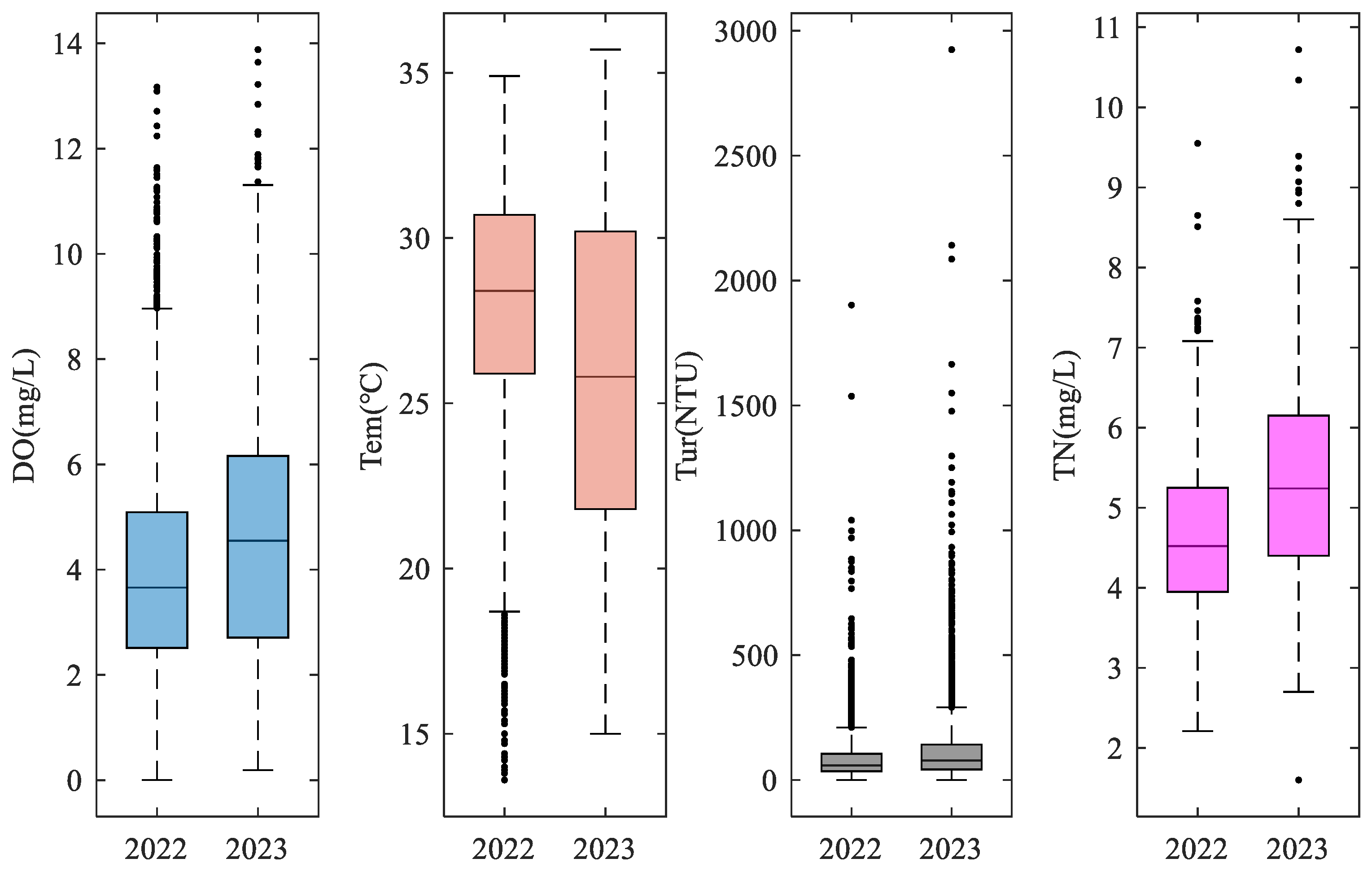
• The pollution loads of BOD, SS, and TN from upstream WWTPs showed significant negative correlations with the daily minimum DO levels at the estuary in 2023, with Pearson correlation coefficients (r) of −0.32, −0.76, and −0.32, respectively. Compared to 2022, these correlations intensified notably, indicating improved water quality in the Shenzhen River after remediation measures in 2023. This enhancement suggests a growing influence of upstream pollutant loads on estuarine hypoxia.

In recent years, the rising frequency of global extreme weather events—particularly marine heatwaves—has intensified the formation of extreme hypoxic events, posing severe threats to estuarine ecosystem security and biodiversity [39]. This study advances our understanding of hypoxia identification in estuarine systems and its driving mechanisms, including the driving effects of key factors such as temperature, Turbidity, and TN, which provides environmental managers with a robust tool for the precise identification of estuarine hypoxia events. Moreover, it delivers critical insights into the time-lagged effects of the driving factors, thereby enabling evidence-based formulation of adaptive management strategies for hypoxia mitigation. Future efforts should focus on enhancing hypoxia forecasting and management through integrated analysis of WWTP discharge data and estuarine water quality monitoring. By quantifying the indirect pathways of key parameters like Turbidity and TN and developing intelligent decision support systems that connect predictive thresholds with early warnings and regulatory actions, this work establishes a foundation for the precision management of estuarine ecosystems. Such advancements will enable a holistic management framework spanning precise early warnings, proactive mitigation, and sustained ecological restoration.

References

1. Grantham, B.A.; Chan, F.; Nielsen, K.J.; Fox, D.S.; Barth, J.A.; Huyer, A.; Lubchenco, J.; Menge, B.A. Upwelling-driven nearshore hypoxia signals ecosystem and oceanographic changes in the northeast Pacific. Nature 2004, 429, 749–754. [Google Scholar] [CrossRef] [PubMed]
2. GB 3838-2002; Environmental Quality Standards for Surface Water. China Environmental Press: Beijing, China, 2002.
3. Liu, S.; Chen, Q.; Hou, C.; Dong, C.; Qiu, X.; Tang, K. Recovery of 1559 metagenome-assembled genomes from the East China Sea’s low-oxygen region. Sci. Data 2024, 11, 994. [Google Scholar] [CrossRef]
4. Engle, V.D.; Summers, J.K.; Macauley, J.M. Dissolved Oxygen Conditions in Northern Gulf of Mexico Estuaries. Environ. Monit. Assess. 1999, 57, 1–20. [Google Scholar] [CrossRef]
5. Schonfeld, A.J.; Ralph, G.M.; Gartland, J.; St-Laurent, P.; Friedrichs, M.A.M.; Latour, R.J. Hypoxia influences the extent and dynamics of suitable fish habitat in Chesapeake Bay, USA. Mar. Ecol. Prog. Ser. 2024, 748, 117–135. [Google Scholar] [CrossRef]
6. Conley, D.J.; Carstensen, J.; Aigars, J.; Axe, P.; Bonsdorff, E.; Eremina, T.; Haahti, B.-M.; Humborg, C.; Jonsson, P.; Kotta, J.; et al. Hypoxia Is Increasing in the Coastal Zone of the Baltic Sea. Environ. Sci. Technol. 2011, 45, 6777–6783. [Google Scholar] [CrossRef] [PubMed]
7. Lee, J.; Park, K.-T.; Lim, J.-H.; Yoon, J.-E.; Kim, I.-N. Hypoxia in Korean Coastal Waters: A Case Study of the Natural Jinhae Bay and Artificial Shihwa Bay. Front. Mar. Sci. 2018, 5, 70. [Google Scholar] [CrossRef]
8. Blaszczak, J.R.; Koenig, L.E.; Mejia, F.H.; Gómez-Gener, L.; Dutton, C.L.; Carter, A.M.; Grimm, N.B.; Harvey, J.W.; Helton, A.M.; Cohen, M.J. Extent, patterns, and drivers of hypoxia in the world’s streams and rivers. Limnol. Oceanogr. Lett. 2023, 8, 453–463. [Google Scholar] [CrossRef]
9. Sheng, H.; Darby, S.E.; Zhao, N.; Liu, D.; Kettner, A.J.; Lu, X.; Yang, Y.; Gao, J.; Zhao, Y.; Wang, Y.P. Anthropogenic eutrophication and stratification strength control hypoxia in the Yangtze Estuary. Commun. Earth Environ. 2024, 5, 235. [Google Scholar] [CrossRef]
10. Xu, H.; Liu, S.; Xie, Q.; Hong, B.; Zhou, W.; Zhang, Y.; Li, T. Seasonal variation of dissolved oxygen in Sanya Bay. Aquat. Ecosyst. Health Manag. 2016, 19, 276–285. [Google Scholar] [CrossRef]
11. Li, D.; Chen, J.; Wang, B.; Jin, H.; Shou, L.; Lin, H.; Miao, Y.; Sun, Q.; Jiang, Z.; Meng, Q.; et al. Hypoxia Triggered by Expanding River Plume on the East China Sea Inner Shelf During Flood Years. J. Geophys. Res.-Ocean. 2024, 129, e2024JC021299. [Google Scholar] [CrossRef]
12. Zhou, J.; Zhu, Z.-Y.; Hu, H.-T.; Zhang, G.-L.; Wang, Q.-Q. Clarifying Water Column Respiration and Sedimentary Oxygen Respiration Under Oxygen Depletion Off the Changjiang Estuary and Adjacent East China Sea. Front. Mar. Sci. 2021, 7, 623581. [Google Scholar] [CrossRef]
13. Howarth, R.; Chan, F.; Conley, D.J.; Garnier, J.; Doney, S.C.; Marino, R.; Billen, G. Coupled biogeochemical cycles: Eutrophication and hypoxia in temperate estuaries and coastal marine ecosystems. Front. Ecol. Environ. 2011, 9, 18–26. [Google Scholar] [CrossRef]
14. Rabalais, N.N.; Cai, W.J.; Carstensen, J.; Conley, D.J.; Fry, B.; Hu, X.P.; Quiñones-Rivera, Z.; Rosenberg, R.; Slomp, C.P.; Turner, R.E.; et al. Eutrophication-Driven Deoxygenation in the Coastal Ocean. Oceanography 2014, 27, 172–183. [Google Scholar] [CrossRef]
15. Caballero-Alfonso, A.M.; Carstensen, J.; Conley, D.J. Biogeochemical and environmental drivers of coastal hypoxia. J. Mar. Syst. 2015, 141, 190–199. [Google Scholar] [CrossRef]
16. Yu, L.; Gan, J. Reversing impact of phytoplankton phosphorus limitation on coastal hypoxia due to interacting changes in surface production and shoreward bottom oxygen influx. Water Res. 2022, 212, 118094. [Google Scholar] [CrossRef]
17. Steckbauer, A.; Duarte, C.M.; Carstensen, J.; Vaquer-Sunyer, R.; Conley, D.J. Ecosystem impacts of hypoxia: Thresholds of hypoxia and pathways to recovery. Environ. Res. Lett. 2011, 6, 025003. [Google Scholar] [CrossRef]
18. Santana, R.; Lessa, G.C.; Haskins, J.; Wasson, K. Continuous Monitoring Reveals Drivers of Dissolved Oxygen Variability in a Small California Estuary. Estuaries Coasts 2018, 41, 99–113. [Google Scholar] [CrossRef]
19. Lin, Z.; Hu, J.; Ye, L.; Cui, Y.; Wu, J. Long-term trends in summer hypoxia and associated driving factors in the Pearl River Estuary, China. Mar. Pollut. Bull. 2025, 211, 117456. [Google Scholar] [CrossRef] [PubMed]
20. Zheng, X.; Liu, H.; Xing, Q.; Li, Y.; Guo, J.; Tang, C.; Zou, T.; Hou, C. Key drivers of hypoxia revealed by time-series data in the coastal waters of Muping, China. Mar. Environ. Res. 2024, 199, 106613. [Google Scholar] [CrossRef]
21. Xu, C.; Luo, P.; Wu, P.; Song, C.; Chen, X. Detection of periodicity, aperiodicity, and corresponding driving factors of river dissolved oxygen based on high-frequency measurements. J. Hydrol. 2022, 609, 127711. [Google Scholar] [CrossRef]
22. Muller, A.C.; Muller, D.L. Forecasting future estuarine hypoxia using a wavelet based neural network model. Ocean Model. 2015, 96, 314–323. [Google Scholar] [CrossRef]
23. Liang, X.; Jian, Z.; Tan, Z.; Dai, R.; Wang, H.; Wang, J.; Qiu, G.; Chang, M.; Li, T. Dissolved Oxygen Concentration Prediction in the Pearl River Estuary with Deep Learning for Driving Factors Identification: Temperature, pH, Conductivity, and Ammonia Nitrogen. Water 2024, 16, 3090. [Google Scholar] [CrossRef]
24. Coopersmith, E.J.; Minsker, B.; Montagna, P. Understanding and forecasting hypoxia using machine learning algorithms. J. Hydroinform. 2010, 13, 64–80. [Google Scholar] [CrossRef]
25. Jiang, Q.; He, J.; Wu, J.; He, M.; Bartley, E.; Ye, G.; Christakos, G. Space-Time Characterization and Risk Assessment of Nutrient Pollutant Concentrations in China’s Near Seas. J. Geophys. Res.-Ocean. 2019, 124, 4449–4463. [Google Scholar] [CrossRef]
26. Gao, K.; Feng, W.; Zhao, X.; Yu, C.; Su, W.; Niu, Y.; Han, L. Anomaly Detection for Time Series with Difference Rate Sample Entropy and Generative Adversarial Networks. Complexity 2021, 2021, 5854096. [Google Scholar] [CrossRef]
27. Torrence, C.; Compo, G.P. A practical guide to wavelet analysis. Bull. Am. Meteorol. Soc. 1998, 79, 61–78. [Google Scholar] [CrossRef]
28. Labat, D.; Ababou, R.; Mangin, A. Rainfall–runoff relations for karstic springs. Part II: Continuous wavelet and discrete orthogonal multiresolution analyses. J. Hydrol. 2000, 238, 149–178. [Google Scholar] [CrossRef]
29. Jiang, J.; Zheng, Y.; Pang, T.; Wang, B.; Chachan, R.; Tian, Y. A comprehensive study on spectral analysis and anomaly detection of river water quality dynamics with high time resolution measurements. J. Hydrol. 2020, 589, 125175. [Google Scholar] [CrossRef]
30. de Boer, P.-T.; Kroese, D.P.; Mannor, S.; Rubinstein, R.Y. A Tutorial on the Cross-Entropy Method. Ann. Oper. Res. 2005, 134, 19–67. [Google Scholar] [CrossRef]
31. Curbani, F.E.; Lacerda, K.C.; Curbani, F.; Barreto, F.T.C.; Tadokoro, C.E.; Chacaltana, J.T.A. Numerical Study of Physical and Biogeochemical Processes Controlling Dissolved Oxygen in an Urbanized Subtropical Estuary: Vitória Island Estuarine System, Brazil. Environ. Model. Assess. 2022, 27, 233–249. [Google Scholar] [CrossRef]
32. Schreiber, T. Measuring Information Transfer. Phys. Rev. Lett. 2000, 85, 461–464. [Google Scholar] [CrossRef] [PubMed]
33. Bharti, V.; Roshni, T.; Jha, M.K.; Ghorbani, M.A.; Ibrahim, O.R.A. Complex network analysis of groundwater level in Sina Basin, Maharashtra, India. Environ. Dev. Sustain. 2024, 26, 18017–18032. [Google Scholar] [CrossRef]
34. Zhu, S.; Zhao, J.; Wu, Y.; She, Q. Intermuscular coupling network analysis of upper limbs based on R-vine copula transfer entropy. Math. Biosci. Eng. 2022, 19, 9437–9456. [Google Scholar] [CrossRef]
35. Kumar, P.; Foufoula-Georgiou, E. Wavelet analysis for geophysical applications. Rev. Geophys. 1997, 35, 385–412. [Google Scholar] [CrossRef]
36. Qian, W.; Gan, J.; Liu, J.; He, B.; Lu, Z.; Guo, X.; Wang, D.; Guo, L.; Huang, T.; Dai, M. Current status of emerging hypoxia in a eutrophic estuary: The lower reach of the Pearl River Estuary, China. Estuar. Coast. Shelf Sci. 2018, 205, 58–67. [Google Scholar] [CrossRef]
37. Luo, L.; Wu, M. Spatiotemporal characteristics of summer hypoxia in Mirs Bay and adjacent coastal waters, South China. J. Oceanol. Limnol. 2023, 41, 482–494. [Google Scholar] [CrossRef]
38. Coogan, J.; Dzwonkowski, B.; Lehrter, J.; Park, K.; Collini, R.C. Observations of dissolved oxygen variability and physical drivers in a shallow highly stratified estuary. Estuar. Coast. Shelf Sci. 2021, 259, 107482. [Google Scholar] [CrossRef]
39. Li, C.; Huang, J.; Liu, X.; Ding, L.; He, Y.; Xie, Y. The ocean losing its breath under the heatwaves. Nat. Commun. 2024, 15, 6840. [Google Scholar] [CrossRef]
Figure 1. Map of WWTP locations, distances to monitoring stations in the SRE, and daily treatment capacities.
Water 17 01862 g001
Figure 2. Comparative boxplot of monitoring dataset parameters in the SRE (January–August 2022 vs. January–August 2023).
Water 17 01862 g002
Figure 3. Demonstration of the potential of CWT to identify anomalies in DO time series.
Water 17 01862 g003
Figure 4. Result of anomaly detection in the 2023 DO time series using Gt.
Water 17 01862 g004
Figure 5. Distribution of DO values during daylight and dark periods in 2022 (left) and 2023 (right).
Water 17 01862 g005
Figure 6. Scatter plot for DO and temperature in 2022 (left) and 2023 (right). Red lines show the linear regression results for the two parameters.
Water 17 01862 g006
Figure 7. Results of anomaly detection in DO and temperature from April to May 2023 using Gt (a) and transfer entropy (TE) between them (b).
Water 17 01862 g007
Figure 8. Observed DO and corresponding DO saturation (induced by temperature) in 2023, the gap between which implies influencing factors other than temperature (upper). Turbidity (gray) and ammonia (magenta) in 2023. Multiple peaks coincide with DO reductions.
Water 17 01862 g008
Figure 9. Results of anomaly detection in DO and Turbidity (a), and TN (c) using Gt and transfer entropy (b,d).
Water 17 01862 g009aWater 17 01862 g009b
Figure 10. Transfer entropy (TE) between Turbidity (a), TN (b), and DO with different time lags in a hypoxia event around 7 April 2023.
Water 17 01862 g010
Figure 11. Time series of DO in the SRE from January to August 2022 (a) and January to August 2023 (e), and the equivalent of daily emission pollution loads of BOD (b,f), SSs (c,g), and TN (d,h) from four WWTPs.
Water 17 01862 g011aWater 17 01862 g011b
Figure 12. Pearson correlation results of equivalent pollutant loads from WWTP4 and daily minimum DO values.
Water 17 01862 g012