Variational Quantum Regression Application in Modeling Monthly River Discharge

Abstract

In the framework of efficient water resources management, the hydrological forecast is the basis of the pertinent management of water resources. Therefore, this study applies the variational quantum regression (VQR), a novel machine learning approach inspired by quantum computing principles, to the series of water discharges from a river in Romania. The models were evaluated against the quantum neural network (QNN) and other classic artificial intelligence (AI) outputs on the same dataset. Performance was assessed based on the coefficient of determination (R²), mean absolute error (MAE), and mean squared error (MSE). VQR outperformed classical neural networks and hybrid models with respect to MSE and MAE, demonstrating superior accuracy and generalization capability. Notably, the models exhibited exceptional skill in capturing monthly maxima—an area where other models often struggle, underscoring the potential of VQR as a powerful and reliable tool for hydrological forecasting, particularly in the context of nonlinear and high-variability data series.

1. Introduction

Reliable hydrological models and the forecasts provided by them are essential to understanding the hydrological processes and efficiently manage water resources [1,2]. Accurately simulating hydrological processes across various spatial and temporal scales remains a central challenge, particularly in the face of increasing climatic variability and anthropogenic influences [3,4,5]. Traditionally, hydrological forecasting has relied on physics-based models (PBMs) and statistical techniques [6,7,8]. The integration of machine learning (ML) models in various domains [8,9,10,11,12,13,14,15] has brought transformative potential to hydrological modeling [16,17,18,19,20,21]. By leveraging vast datasets and learning from patterns within them, AI models can enhance forecasting accuracy, reduce computational demands, and provide real-time adaptability. ML models are more efficient in computational terms and need a reduced amount of data and characterization of the studied case when compared to PBMs.

Variational quantum regression (VQR), a variational quantum algorithm (VQA), is commonly used for regression problems. Its principle is based on the variational method, where a quantum state with variational parameters is constructed, and classical optimization algorithms iteratively adjust these parameters to minimize the difference between an observable quantity and the target value [22,23]. In VQR, a quantum state (parameterized by variational parameters) is first prepared, followed by measurements, to obtain the estimated value of a record. The variational parameters are further updated by a classical optimizer that considers the discrepancies between the simulated and target values. The process is repeated until an optimal solution is found.

The variational quantum circuits (VQCs) involved in quantum computation demonstrated performance comparable to classical neural networks on supervised and reinforcement learning tasks, utilizing significantly fewer trainable parameters [24,25,26]. Unlike classical models, which rely on kernel tricks to manage computational costs, quantum circuits directly leverage quantum resources to model functions intractable for classical systems [27]. Although VQCs currently involve longer training durations, their parameter efficiency highlights their potential as an alternative with high potential for specific machine learning applications [28].

Practical implementation of VQR faces challenges. As problem complexity increases, quantum circuit depth and complexity grow rapidly, exacerbating computational burden and error accumulation, which can diminish accuracy [29]. Furthermore, selecting appropriate variational forms and optimization algorithms is critical to VQR performance (yet no universal method exists), requiring problem-specific investigation and fine-tuning [22]. However, VQR has demonstrated potential in various scientific and industrial domains [30,31,32,33,34,35,36,37,38,39]. It offers a promising framework for learning nonlinear and complex mappings in data-rich environments by exploiting quantum superposition and entanglement, which allows for more effective modeling of complex patterns compared to classical methods [37].

The bibliographical search on quantum computing applications in Environmental Sciences and Geosciences returned only a few results [40,41,42,43]. Berger et al. [41] identified four critical areas where quantum technologies could have high-impact applications: simulating physical systems, combinatorial optimization, sensing, and energy efficiency. Their work emphasizes the need for interdisciplinary collaboration to explore these opportunities. Ahmad and Jas [42] introduced a quantum temporal convolutional network model targeting PM_2.5 levels in highly polluted regions. Their approach demonstrated improved predictive accuracy over traditional models. Grzesiak and Thakkar [43] explored the application of quantum machine learning in flood prediction, which integrates quantum algorithms with classical machine learning techniques. Their hybrid model achieved competitive training times and improved prediction accuracy for daily flood events along Germany’s Wupper River.

Given the limited literature on hydrological modeling using quantum computing and the findings that VQR can provide compressed and nonlinear regression mappings in domains involving signal processing [44] (univariate time series might be considered nonlinear signals), we developed three VQR-based models for monthly river discharge data from 1955 to 2010 from the Buzău River (Romania). This study aimed to evaluate the suitability of VQR for hydrological forecasting by benchmarking the models against previous results obtained from classical approaches on the same dataset. The motivation stemmed from the inability of traditional AI and hybrid models to accurately predict monthly discharge values, especially in months with high water and floods. Our findings demonstrate that the quantum models outperformed classical neural networks and hybrid models, highlighting VQR’s potential advantages in this domain.

2. Materials and Methods

2.1. Study Region and Data Series

The Buzău River (Romania) springs about 1800 m north of the Ciucaș Mountains. It has a direction from north to south and is 334.4 km long [45,46]. The river’s hydrographic basin (h.b.) (Figure 1) is situated in the eastern part of Romania, within the Carpathian region, with an area of 5264 km². The Buzău River drains into the Siret, a main Danube tributary.

The river basin altitude varies from 114 m to 1915 m. Upstream Nehoiu, the catchment is characterized by steep slopes and a predominantly torrential hydrological regime. The average slope is about 11.7° in the upper and middle of h.b. Some parts of the catchment are covered by forest, with afforestation coefficients between 23% (Câlnău) and 84% (Bâsca Mare) [47]. Coniferous, broad-leaved, and mixed forests cover 41% of the study zone. Approximately 33% of the area is occupied by pastures, arable fields, and orchards [48], mainly in the southern part. Flysch formations, with heights between 900/1000 and 1700 m, are found in Carpathian regions. The Subcarpathians are made up of soft rock layers, mostly marl and clays, and rise to 900 m high. Clay-rich rocks from the Neogene period, containing minerals like montmorillonite and illite, are common at the surface. These soft materials cause the slopes’ instability, so landslides often occur. The most frequent types are shallow slides, deeper rotational slides, and mudflows [49]. The region exhibits a humid continental climate with significant seasonal and interannual variability in precipitation, often leading to rapid runoff and frequent flash flood events [50,51].

These hydrological dynamics make catchment a critical area for flood risk assessment and hydrological modeling. The catchment is relatively well-instrumented, with several hydrometric stations providing long-term flow and rainfall data, making it a valuable case study for testing advanced forecasting and modeling techniques [52,53,54].

Due to its complex topography, heterogeneous land cover, and sensitivity to climate event variation, the Buzău Catchment has been the focus of numerous hydrological studies, particularly those related to runoff generation, flood forecasting, and the evaluation of climate change impacts mountainous water systems [55,56,57].

The Buzău River has experienced several major flood events over the past decades, with the most significant ones occurring in 1970, 1972, 1975, 1988, 1991, and 2005. The 1970s were particularly notable, with eight major floods and the highest average annual peak discharge for the decade (853 m³/s). In contrast, the following decades—1980–1989 and 1990–2000—saw a marked reduction in flood frequency and intensity. However, this trend reversed in 2000–2010. The highest flood occurred in July 1975, when the discharge peaked at 2100 m³/s. In comparison, during the July 2005 floods, the maximum discharge was significantly lower—925 m³/s—primarily due to the attenuating effect of the Siriu and Cândești reservoir dams constructed upstream [57]. In January 1984, the dam on the Buzău River at Siriu was partially commissioned, with the primary objectives of hydroelectric power generation and flood control.

The dataset analyzed consists of monthly river flow records spanning January 1955–December 2010, called S in the following, was divided into subseries S1 and S2, before and after January 1984. The records originated from the National Institute of Hydrology and Water Resources Management, where they were checked for accuracy. The series had no missing values.

Three models were developed: M was trained on data up to January 2005, M1 used series S1 for training, and M2 was trained on data from January 1984 to December 2005. In all cases, forecasting was performed on a common test set starting from January 2006. At the second study stage, other models, Mo, Mo1, and M2o, were built using the anomaly-filtered version of the series, called So, S1o, and S2o. The anomalies are presented in the Tables from Figure 1. Their detection was presented in detail in article [54]. The training and test sets covered the same period as in the case of models M, M1, and M2.

2.2. Basic Concept of Variational Quantum Regressor and VQR Structure

The qubit is the equivalent of a bit in classical computing. It is a 2D quantum system whose state can be written as:

|𝜙⟩ = 𝛼 |0⟩ + 𝛽 |1⟩

(1)

where

$$|0⟩=\left(\begin{array}{c}1\\ 0\end{array}\right), 𝛽 |1⟩=\left(\begin{array}{c}0\\ 1\end{array}\right)$$

(2)

and the complex numbers α and β satisfy

$${\alpha }^2+{\beta }^2=1.$$

(3)

VQR is a quantum regression model based on a VQA. By leveraging the parameterized nature of variational quantum circuits (VQC), VQR achieves nonlinear mapping and optimization of input data, enabling regression tasks [23]. This approach combines quantum parallelism and classical optimization techniques, aiming to exploit quantum computing’s potential advantages in high-dimensional feature mapping and computational efficiency, thereby enhancing regression modeling capabilities.

VQR relies on the following operations and elements:

• Feature encoding, which transforms the input data into quantum states;
• The variational quantum circuit (VQC) that uses parameterized quantum gates to perform quantum state transformations;
• Measurement and optimization, which extract output results via quantum measurement and optimize the circuit parameters using classical methods to achieve model convergence.

VQR performs regression tasks using a parameterized quantum circuit, with its core structure comprising [58]:

• Quantum feature encoding: classical input data must be transformed into quantum states for quantum computation. This encoding process is typically performed using parameterized quantum gates (e.g., $R_y$, $R_z$, ZZ-interaction gates). For an input x, the encoding can be represented as the following:

  $$\left|\psi \left(x\right)⟩=R_y\left(x\right)\left|0⟩\right.\right.$$

  (4)

  where $\psi$ is a state. In multi-qubit systems, quantum entanglement (e.g., ZZ interaction) can be utilized to enhance feature representation.
• Quantum processing: during this process, a VQC is applied to transform the quantum state. The VQC serves as the core of the VQR and consists of parameterized quantum gates and entangling gates akin to the hidden layers in classical neural networks. The VQC learns feature representations from the input and optimizes the trainable parameter θ by [58]:

  $$U\left(\theta \right)=R_y\left({\theta }_1\right)R_z\left({\theta }_2\right)CNOT$$

  (5)

  where CNOT gates introduce quantum entanglement, and multiple circuit layers enable the modeling of complex nonlinear mappings.
• Measurement and regression computation: since quantum computation results are stored in quantum states, quantum measurement is required to extract information. VQR applies Pauli-Z measurement to compute the expectation value of the quantum state by:

  $$f\left(x,\theta \right)=⟨\psi \left(x,\theta \right)|Z|\psi \left(x,\theta \right)⟩$$

  (6)
  Due to the probabilistic nature of quantum measurements, shot-based sampling is typically employed to reduce measurement errors and improve result stability.
• Loss computation using the standard loss functions:

  $$\mathrm{M}\mathrm{S}\mathrm{E}={\displaystyle \frac{1}{N}}\sum _{i=1}^N{(f\left(x_i,\theta \right)-y_i)}^2$$

  (7)

  $$\mathrm{M}\mathrm{A}\mathrm{E}={\displaystyle \frac{1}{N}}\sum _{i=1}^N\left|f\left(x_i,\theta \right)-y_i\right|$$

  (8)
• Parameter optimization: the process uses classical algorithms (e.g., L-BFGS-B [59,60], COBYLA [61,62], and Adam [63]) to optimize the parameters of quantum circuits using the equation:

  $${\theta }_{t+1}={\theta }_t-\eta {\nabla }_{\theta }L\left(\theta \right)$$

  (9)

  where η is the learning rate.
  The parameter θ is optimized through iterative training to minimize the regression error and finally obtain the optimal model.

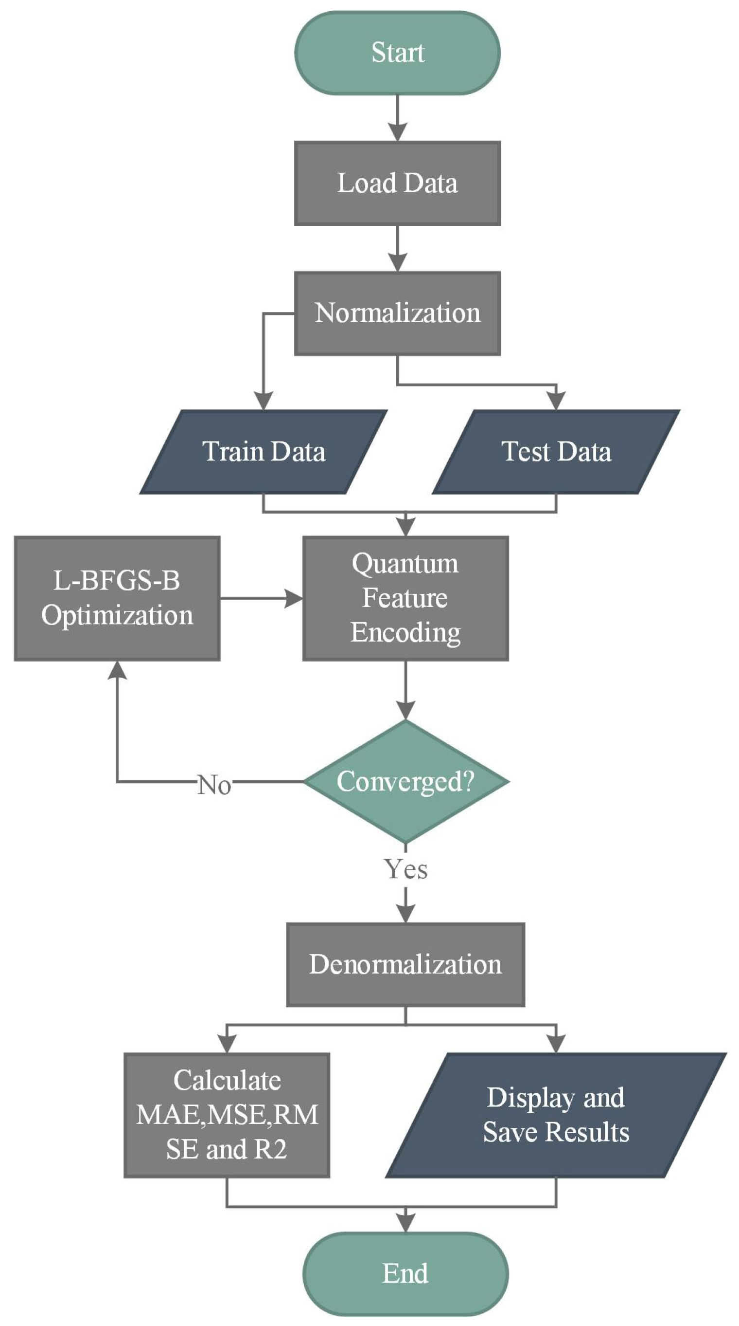
2.3. Modeling Stages

The modeling stages of the study are as follows.

1.

Load data and preprocessing:

• Raw data was imported, checked for missing values and outliers, and normalized. No cleaning was necessary given the series origin and accuracy.
• The normalized series were split into training and test sets.

2.

Quantum feature encoding and circuit design

• Training data are encoded via a single-qubit feature map.
• A variational ansatz circuit is constructed.

3.

Optimization loop

• The L-BFGS-B optimizer iteratively updates circuit parameters.
• A convergence check directs the loop until stopping criteria are met.

4.

Post-processing and evaluation

• Optimized outputs are de-normalized.
• Standard goodness-of-fit metrics (MAE, MSE, RMSE, R²) are calculated.
• Results are displayed and saved for further analysis.

The study flowchart is shown in Figure 2.

Table 1. Parameters settings.

Hyperparameter	Description
Number of qubits	1
Quantum register	1 qubit
Classical register	0 bits
Feature map	QuantumCircuit(1, name=“fm”), with an ry(param_x) rotation on qubit 0
Variational circuit (ansatz)	QuantumCircuit(1, name=“vf”), with an ry(param_y) rotation on qubit 0
Optimizer	L_BFGS_B(maxiter=50)
Callback	callback_graph, used to record the objective function value at each training iteration
Estimator	EstimatorQNN(circuit=qc, estimator=estimator): StatevectorEstimator
Loss function	MSE
Training call	vqr.fit(X_norm, y_norm), fitting the model on normalized inputs and targets

contains the parameters settings.

The experiments were conducted on a computer with an AMD RYZEN5 5500 processor (AMD, Santa Clara, CA, USA) and 24 GB RAM. Anaconda was used to manage the Python 3.12 environment and dependencies. Modeling was carried out using IBM’s Qiskit framework. Additional libraries, including SciPy and NumPy, were employed to enhance computation performance and stability.

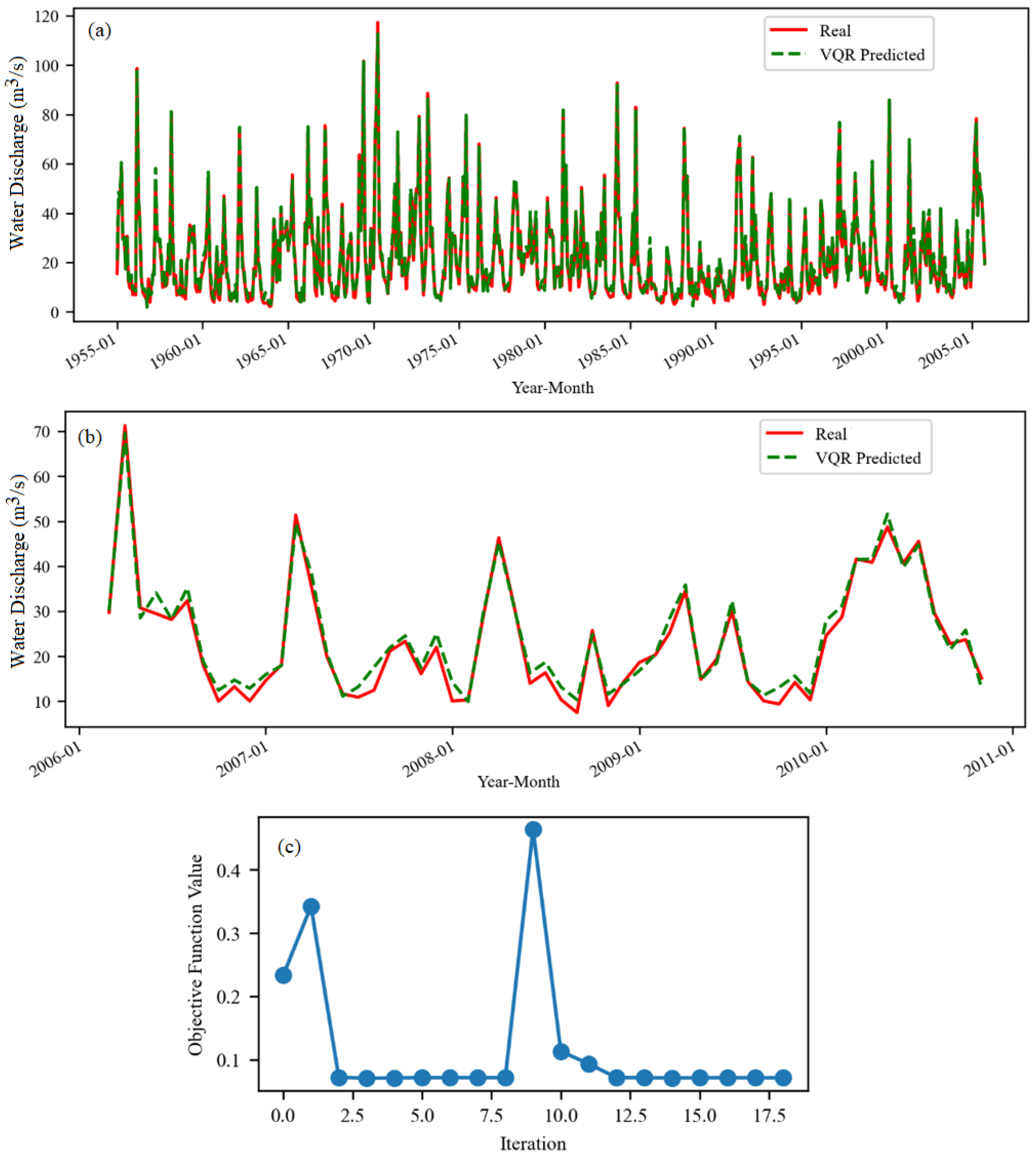
3. Results

The series chart is presented in Figure 1, and the basic statistics of the S, S1, and S2 are presented in Figure 3a,b. Figure 3c contains the violin plot.

3.1. Models for Initial Datasets

Figure 4a, Figure 5a and Figure 6a display the recorded and computed values on the training sets of the models M, M1, and M2. A visual examination of these charts reveals no significant discrepancies between the recorded and estimated series, suggesting a good fit for the raw data. The computed and observed series exhibit similar overall patterns. Model M generally overestimates the recorded data, while M1 and M2 systematically underestimate it. Nonetheless, all models successfully capture the peak values.

Figure 4b present the recorded values from the test sets, alongside the estimated values produced by the M model using the VQR technique. Figure 4c displays the variation in the objective function over 18 training epochs. Some discrepancies between the initial and computed series trends are noticed on the test set of M model (Figure 4b) from March 2006 to May 2006, with a higher variation in the predicted than in the recoded values. During April–June 2007, the variability of the recorded series is lower than those of the registered data. In both cases, the consequence is an increase in the estimation error compared with the other segments in the test period.

The test set chart and corresponding forecasts for model M1 (Figure 5b) reveal the largest deviations between recorded and predicted values during the periods of November 2008 to March 2009 and after March 2010. Comparisons with Figure 4b, which presents the results for Model M, confirm these observations by indicating smaller deviations in the latter case. This finding is particularly relevant given that both models share the same test set, highlighting the importance of identifying the model that delivers the most accurate forecast for the test period.

The comparison of Figure 6a with Figure 4a and Figure 5a reveals greater biases between the recorded and simulated values on the training set in M2, suggesting a less effective learning process in this model compared to M and M1. This may imply a potentially reduced prediction accuracy on the test set, where the model applies its learned patterns. However, Figure 6b highlights the highest alignment between the shape of the test set and the forecast in M2, indicating better performance in capturing the trend dynamics during January 2006 and December 2010 relative to M and M1.

In Figure 4c, Figure 5c and Figure 6c, we remark that after the first iteration, the values of the objective function increased to double, then leveled off below 0.1. At the ninth (eleventh and ninth, respectively) iteration, the objective function reaches its maximum, then decreases again to reach the minimum, under 0.1.

Visual assessments must be complemented by numerical evaluation to objectively measure model accuracy. Accordingly, the performance of the VQR models was assessed using three goodness-of-fit metrics: mean absolute error (MAE), mean squared error (MSE), and the coefficient of determination (R²). The corresponding values for each model are reported in

Table 2. Goodness-of-fit indicators in models M, M1 and M2.

Model	Set	MAE	MSE	R2
M	Training	1.5158	3.6647	0.9886
	Test	1.7197	4.335	0.9742
M1	Training	2.3706	8.3552	0.9767
	Test	2.1569	7.3694	0.9561
M2	Training	2.4182	7.6084	0.9728
	Test	2.2678	6.8897	0.9589

.

Across all three indicators, M demonstrated the best overall performance, achieving the lowest MAE and MSE, as well as the highest R² on both the training and test sets. In terms of MAE, M1 ranked second, while considering MSE, M2 outperformed M1. With respect to R², M1 held the second-highest value, but only on the training set. Nevertheless, the R² values for M1 and M2 were relatively close, indicating comparable explanatory power.

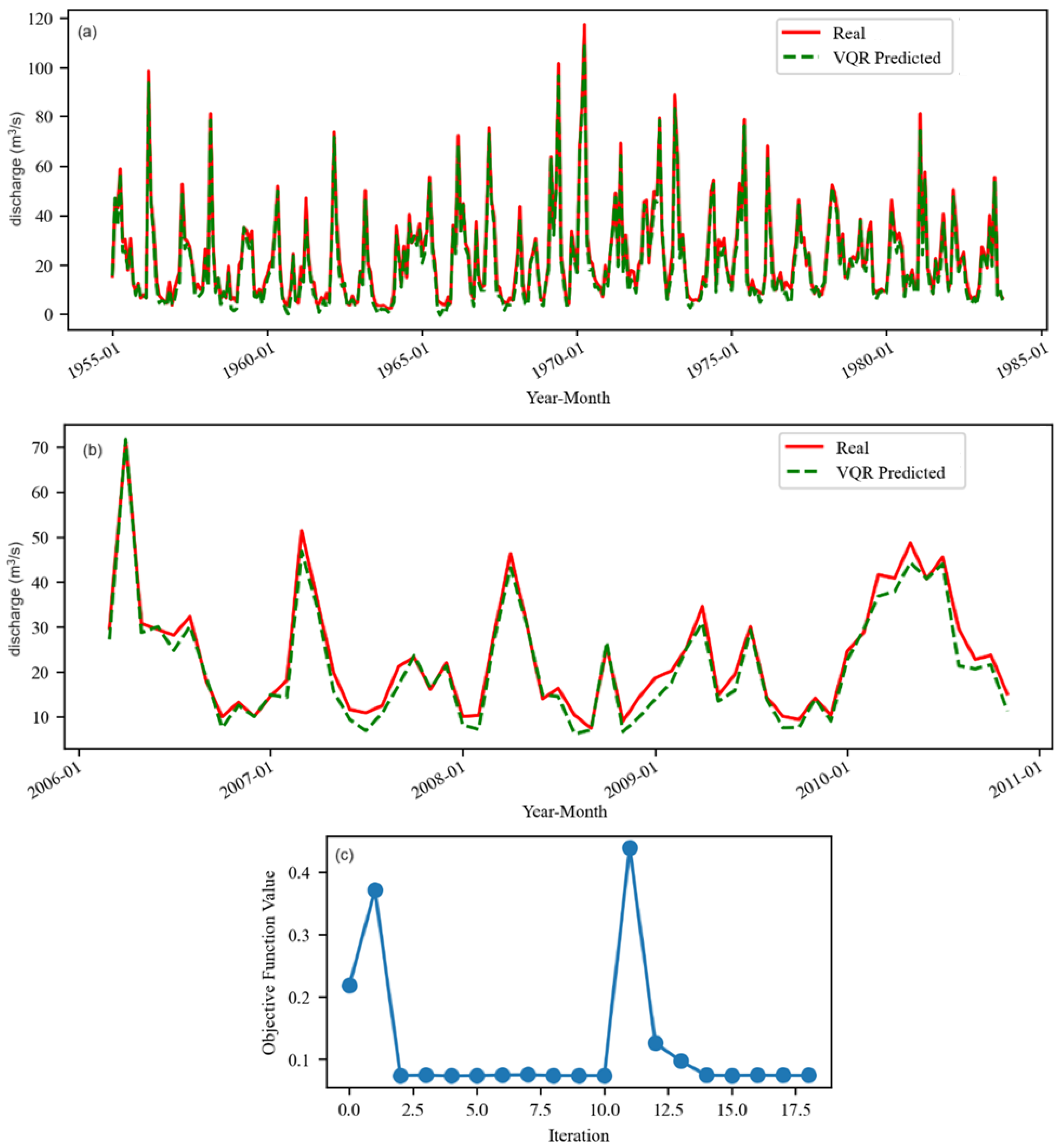
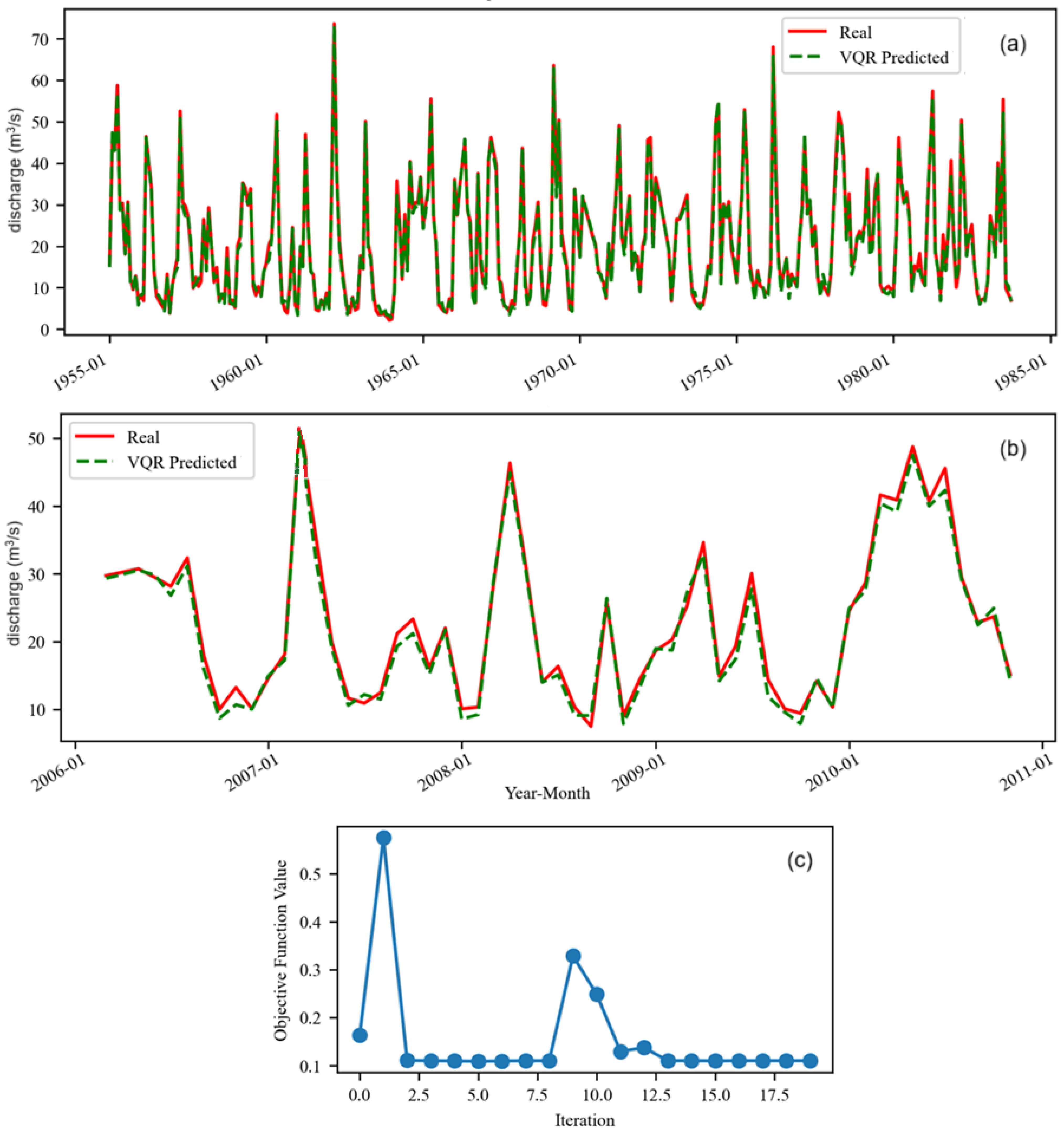
3.2. Models for the Series Without Aberrant Values

In the second stage of the analysis, we excluded the aberrant values (indicated in Figure 1) and ran the VQR the algorithms on the adjusted series. This step aimed to evaluate the performance of the VQR on more homogeneous hydrological series. However, it is important to emphasize that the aberrant values may correspond to significant flood events with high return periods. Therefore, they must be retained when applying the models, as was performed in Section 3.1. The results of models Mo, M1o, and M2o are represented in Figure 7a, Figure 8a and Figure 9a for the training sets, and Figure 7b, Figure 8b and Figure 9b for the test sets.

Comparing the charts in Figure 4 and Figure 7, a better fit of the recorded values—particularly on the test set—is observed in the Mo compared to the M. During the second iteration, the objective function rose to 0.58 before stabilizing around 0.12. This value remained relatively constant until the 12th iteration, at which point it abruptly rose to approximately 0.35. Following the 16th iteration, the objective function plateaued near 1.2. This pattern is like the behavior observed when the algorithm was applied to series S, with a similarly noticeable increase occurring around the 12th iteration.

An analysis of Figure 5 and Figure 8 shows that the M1o offers a superior fit, especially in accurately capturing both the minimum and average discharge values. It also shows improved agreement between the observed and simulated trend patterns.

The objective function for the M1o declined after the second iteration and then stabilized around 0.1. Although this value remained constant, it is slightly higher than the minimum achieved in M1.

A comparison of Figure 6b and Figure 9b reveals that the M2o exhibits significantly larger biases than the M2. The objective function values remained nearly constant at approximately 0.05 between the second and eighth iterations, and again from the thirteenth iteration onward, indicating a convergence pattern similar to that observed in the Mo and M1o. Although peak values were estimated with reasonable accuracy, M2o demonstrated the weakest overall performance, with a pronounced overestimation of the observed values.

Table 3. Goodness-of-fit indicators in Mo, M1o, and M2o.

Model	Set	MAE	MSE	R2
Mo	Training	0.9559	1.4420	0.9919
	Test	1.0103	1.5313	0.9881
M1o	Training	1.0585	1.8321	0.9906
	Test	1.1503	1.9007	0.9853
M2o	Training	2.8241	9.0615	0.9454
	Test	2.5055	7.5413	0.9416

presents the goodness-of-fit indicators and their corresponding values for the Mo, M1o, and M2o to enable a proper comparison. Comparisons between the models trained on the raw series and those trained on the series with aberrant values removed indicate improved accuracy for both the Mo and M1o relative to M and M1, respectively. This is particularly evident in terms of MSE, which decreased by at least a factor of 2.5. In contrast, M2o demonstrated the poorest performance among all variants.

4. Discussion

4.1. Discussions on Modeling Results

Some results from the VQR models were unexpected for the following reasons:

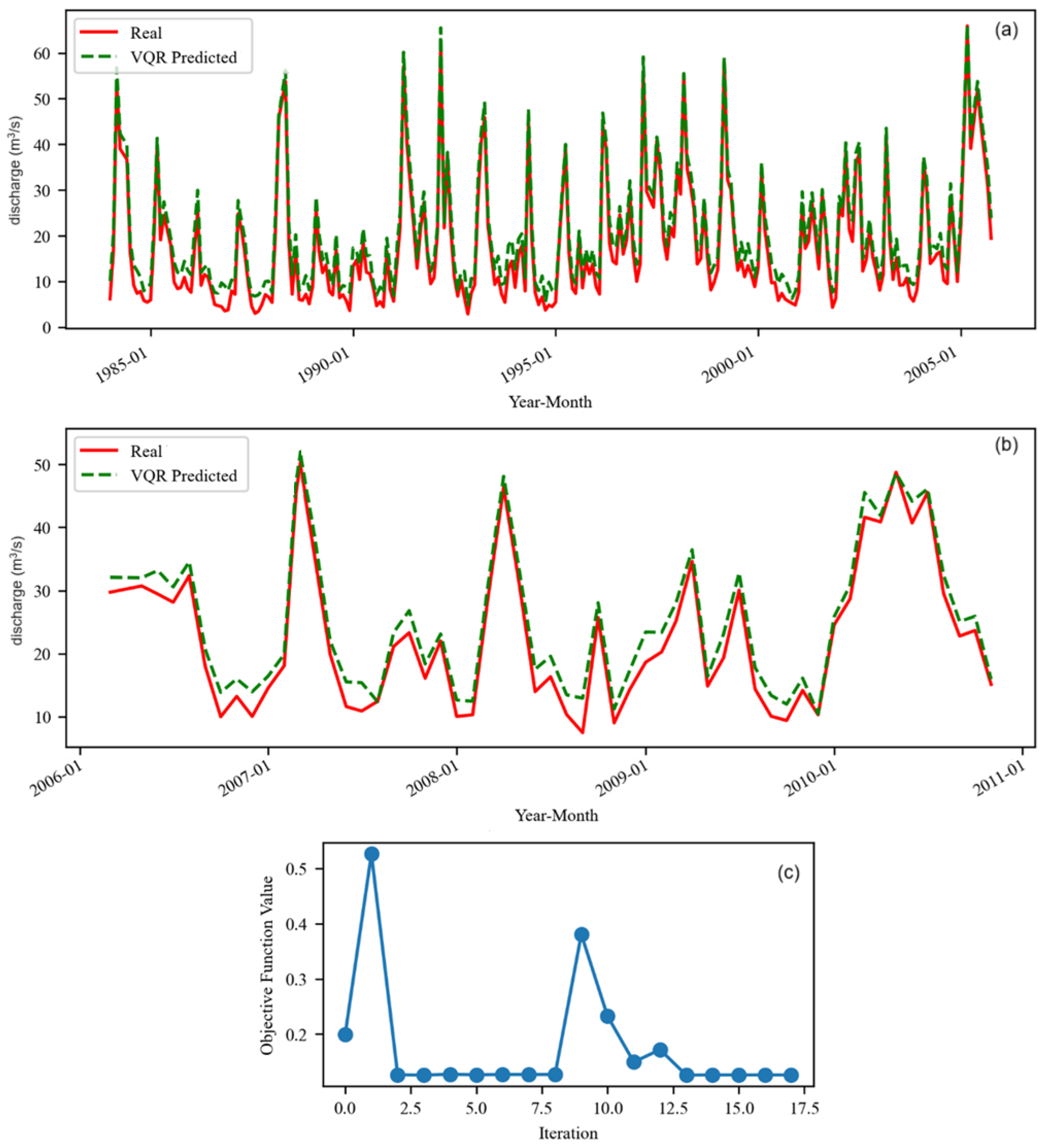
• The data series comprises discharge values recorded over two distinct periods: before and after the dam’s construction. Prior to January 1984, the series features numerous high-peak floods that significantly elevated the monthly average discharge. Following January 1984, a marked reduction in both the frequency and intensity of floods was observed, leading to decreased variability in average discharge. Previous studies [51,52,53] have demonstrated that the subseries corresponding to the pre- and post-dam periods exhibit different statistical behaviors.
• In M2, both the training and test sets belong to the post-1984 period. As a result, the model was expected to generalize well, applying learned patterns effectively within the same hydrological regime.
• M1 was trained on data from the pre-1984 period and tested on data from the post-1984 period. Despite the distinct differences in flow patterns between the two sub-periods, it outperformed M2. This suggests that the richer variability and more dynamic patterns in the pre-1984 data may have enabled the model to learn more robust or generalizable features, even when applied to a different hydrological regime. This finding is contrary to the output of other kinds of neural networks and hybrid models [52,53,54].
• M was trained on a subseries that spans both the pre-1984 and 1984–2005 periods, allowing it to learn patterns from both the unregulated and regulated flow regimes. It was then applied to a post-2005 subseries, which exclusively reflects the regulated flow conditions. It seems that M, benefiting from richer temporal coverage and greater variability in its training data, enabled stronger generalization to post-2005 conditions.
• All classical neural network models built on the same data series with the same training and test sets demonstrated better performance on more homogeneous time series. Therefore, it was expected that M2o would perform better than M2, but this was not the case.

The length of the series appears to influence the performance of the VQR output, with M (trained in the longest series) showing the best results, and the M2 (trained in the shortest series) performing the worst. However, this observation remains preliminary, and more extensive studies are required to rigorously validate the impact of series length on model performance.

The time complexity was in this study O(τBpT_c′), where

• τ = number of iterations, set by maxiter in the optimizer
• B = mini-batch size (in this case it was equal to the data size = n)
• P = circuit depth (the number of gate layers that must be executed sequentially)
• T_c′ = time per circuit when using the StatevectorEstimator.

The method did not incur an O(n³) computational cost with respect to the total sample size n, instead maintaining a polynomial dependence on the number of circuit parameters and measurement efforts. It effectively leverages an exponentially large feature space without the need to explicitly construct or store an exponentially large kernel matrix. This characteristic highlights the potential of VQR for applications involving high-dimensional feature spaces, as is the case in this study.

Table 4. Runtime and number of epochs until convergence on the training sets.

Model	Time(s)	Epochs	Model	Time(s)	Epochs
M	21.8606	30	Mo	14.3117	25
M1	5.168	18	M1o	6.8727	19
M2	4.6312	17	M2o	4.3097	17

contains the runtime of the VQR algorithm, along with the number of epochs required for convergence during training. In general, longer or more complex time series tend to require increased computation time. However, this assumption does not entirely hold in our case. Although M and Mo exhibited the highest runtimes, the runtime for M1o exceeded that of M1, even though M1o was trained on a shorter time series.

A similar pattern was observed in the number of epochs needed to reach the optimum of the objective function: 30, 18, and 17 epochs were required for the raw series in M, M1, and M2, respectively. In contrast, the number of epochs decreased for models Mo and M2o, while it slightly increased for M1o.

4.2. Assessment of Fitting Quality of Aberrant Values

An important direction for future research is the evaluation of network performance specifically on extreme values. Based on the results obtained of the models for the raw series, we determined the MAE, MSE, and R² corresponding only to the aberrant values. Note that only one such value belongs to the test set; therefore, we report the goodness-of -fit indicators from the training test only. They are as follows:

• In M: MAE = 1.6851, MSE = 2.1199, R² = 0.9814
• In M1: MAE = 4.0440, MSE = 4.2410, R² = 0.9917
• In M2: MAE = 3.7306, MSE = 4.083 R² = 0.9824.

It is worth noting that all models provided a good fit for the aberrant values. Based on MAE and MSE metrics, M performed best, followed by M2 and M1. However, when considering the R² coefficient, the best fit was achieved by M1, with M2 and M following in performance.

4.3. Comparisons of the VQR Models’ Performance with Those of Classical Artificial Neural Networks and Quantum Neural Networks

In previous studies, we evaluated the effectiveness of artificial neural networks (ANNs) for modeling river discharge using the same dataset. The classical ANNs applied to the same series, and same training and test sets, included Backpropagation Neural Networks (BPNNs), Convolutional Neural Networks (CNNs), Echo State Networks (ESNs), Extreme Learning Machines (ELMs), Long Short-Term Memory (LSTM) networks, and Multilayer Perceptrons (MLPs). Additionally, we explored several hybrid ANN architectures, such as CNN-LSTMs, Particle Swarm Optimization with Extreme Learning Machines (PSO-ELMs), Sparrow Search Algorithm with Backpropagation Neural Networks (SSA-BPs), and Sparrow Search–Echo State Network (SSA-ESN). For details, the reader can see articles [51,52,53]. The best-performing models are summarized in

Table 5. Goodness-of-fit indicators for the best classical AI and hybrid models.

Model	Set	MAE (Model)	MSE (Model)	R2 (Model)
M	Training	5.7250 (SSA-BP)	80.5765 (ESN)	0.9976 (SSA-ESN)
	Test	4.2351 (CNN-LSTM)	32.4993 (SSA-BP)	0.9983 (LSTM)
M1	Training	6.5177 (CNN-LSTM)	102.9393 (ESN)	0.9899 (LSTM)
	Test	4.4784 (CNN-LSTM)	39.7982 (CNN-LSTM)	0.9917 (LSTM)
M2	Training	4.7433 (CNN-LSTM)	57.3421 (SSA-ESN)	0.9992 (LSTM)
	Test	3.5245 (CNN-LSTM)	29.8323 (CNN-LSTM)	0.9970 (LSTM)

.

The results in Table 2 and Table 5 indicate that VQR outperformed other models in terms of MAE and MSE. In terms of the R² metric, the best-performing algorithm was SSA-ESN on the training set and LSTM on the test set of the S series, while LSTM achieved the highest R² for M1 and M2. The ESN model recorded the shortest runtime, completing in under 0.65 s. A comparative analysis between VQR and quantum neural networks (QNN) [64] on the raw series reveals that:

• When using QNN, the number of epochs to reach the objective function optimum was the lowest (9 epochs for S, 11 for Mo, 10 for M1 models, and 8 epochs for M2, M1o, and M2o models);
• When applying VQR, the smallest runtime was recorded on M1 (5.168 s) and M2o (4.3097 s) models, while running QNN resulted in shorter runtimes on M (10.8472 s), M2 (4.6218 s), Mo (12.1807 s), and M1o (5.5552 s) models.
• VQR achieved the best performance on the M model training set, while QNN produced the best results on the test set, with MAE = 1.1937, MSE = 2.3815, and R² = 0.9858;
• VQR showed superior performance compared to QNN on M1, M2, Mo, and M2o, whereas QNN outperformed VQR on M and M1o.
• QNN performed better than ESN and SSA-ESN on the series without aberrant values in terms of MSE and MAE. On So and M2o, ESN was the best with respect to R² on the test set. Moreover, the time necessary to run the algorithms was significantly lower for ESN and SSA-ESN.

To assess and compare the performance of previously studied AI models with those of VQR, we employed graphical representations. Figure 10 illustrates these comparisons: the Taylor diagram, diagram on the left shows the results for the M model on the training set, using VQR as the reference, while the radar plot on the right offers a comprehensive overview of performance metrics.

From the Taylor diagram, the results show that:

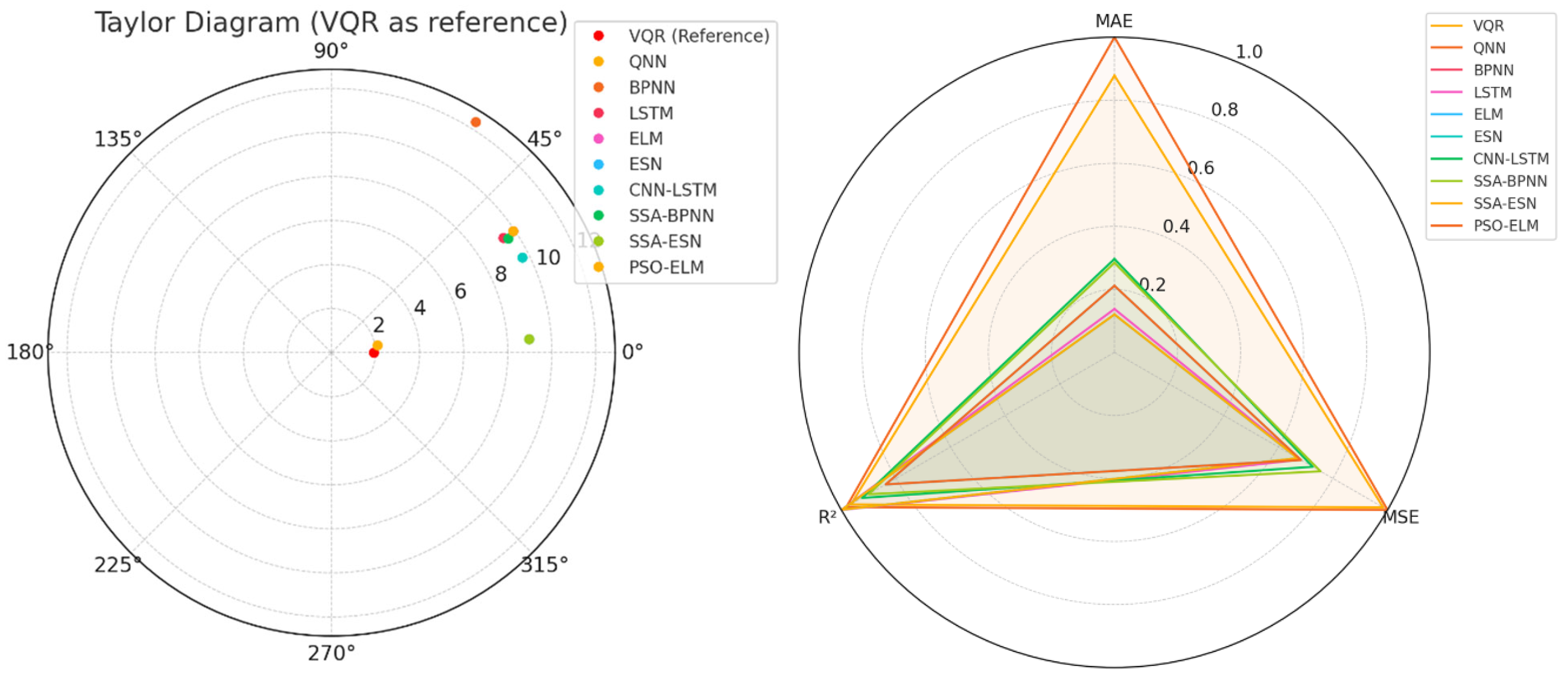
• VQR, QNN, and SSA-ESN are the closest to the reference point, indicating the best performance.
• BPNN stands out with a high standard deviation and low correlation, showing its weak performance.
• ESN and SSA-ESN show high correlation and reasonable variance, performing very well.

From the radar plot it results in that

• QNN, VQR, and SSA-ESN show strong performance across all metrics.
• BPNN performs the worst, especially on MSE and R².
• LSTM and CNN-LSTM also perform well, particularly on R².

4.4. Limitations of the Actual Study

Despite the promising results of the VQR models, this study has several limitations, leaving a lot of space for improvement. First, all quantum experiments were conducted using classical simulations within the Qiskit framework, given current hardware constraints. Therefore, the results do not account for the noise and error rates inherent in real quantum devices, which could impact the models’ performance.

Moreover, while the quantum model demonstrated superior predictive accuracy compared to classical and hybrid neural networks, this study does not provide a formal theoretical justification for the observed performance gains. Therefore, the conclusions are based on empirical comparisons and cannot be generalized for all hydrological modeling tasks.

A comprehensive study of VQR’s optimization dynamics is also needed. Future efforts will employ loss landscape visualization, Hessian spectral analysis, and quantum Fisher information metrics to examine how initialization schemes, batch size, and measurement repetitions influence convergence speed and stability.

Deriving worst-case and average-case complexity lower bounds for VQR using quantum information complexity theory and quantifying encoding efficiency and generalization limits via quantum mutual information and quantum Fisher information will also highlight the extent of VQR performances for the problem at hand.

Beyond the L-BFGS-B optimizer and single-layer R_y circuit used here, alternative classical and quantum optimizers (e.g., Adam, SPSA, quantum natural gradient) should be evaluated. Systematic comparisons of variational ansatz designs—such as multi-layer circuits, parameter-sharing topologies, and domain-informed feature maps—will identify the architectures that best balance expressive power and trainability.

5. Conclusions

In this article, we evaluated the VQR’s capability to forecast the water flow of the Buzău River. The findings indicate that VQR performed better than other NN and hybrid techniques in terms of MAE and MSE, effectively improving the evaluation of the maxima values of the water discharge. It should be noted that, in hydrology, keeping the maxima in the analysis is necessary given that they indicate exceptional phenomena. In this context, the results’ accuracy is remarkable. However, the study was also performed after the aberrant values’ removal to determine the models’ performances when the series variability is lower. This process significantly enhanced series prediction accuracy, particularly in the M1 and M2, where the models exhibit notably improved generalization. Among the datasets, the highest prediction accuracy was achieved on Mo, followed by M1o.

Comparing the forecast provided by VQR with those obtained by other simple and hybrid models, except QNN, indicates the best accuracy provided by the former algorithm. Comparisons between VQR and QNN indicate that both algorithms exhibit high computational efficiency and perform better on longer datasets (e.g., S dataset), enabling fast convergence and relatively accurate predictions. For more complex datasets (e.g., S, S1o), QNN demonstrates superior predictive accuracy and robustness, particularly in handling outliers. Comparing the algorithms that gave the best results on the study series (LSTM, CNN-LSTM), one may notice that their run time was much lower than that for the quantum algorithms. Therefore, in practical applications regarding river water discharge, the choice of model should depend on the purpose of the study.

The findings of this study provide valuable insights into the applicability of quantum-based models in hydrological forecasting. They highlight the importance of dataset complexity and outlier management in predictive modeling.

Future studies should aim to test VQR models on actual quantum hardware, particularly as devices continue to improve in terms of coherence time, gate fidelity, and qubit count. Investigating alternative data encoding strategies—such as amplitude encoding or hybrid quantum–classical schemes—may improve the scalability and effectiveness of quantum models on larger and more complex hydrological datasets.

Furthermore, a theoretical analysis of VQR’s representational power and generalization capacity in the context of nonlinear hydrological series would strengthen the foundation of quantum-based approaches for such modeling.

Applying VQR to multivariate hydrological time series and incorporating environmental predictors such as precipitation, snowmelt, and temperature could enhance model robustness. Moreover, comparative studies involving quantum-inspired algorithms and hybrid neural network architectures may offer further insight into the conditions under which quantum models provide real advantages in environmental modeling.

References

- Cristian, A.; Zuzeac, M.; Ciocan, G.; Iorga, G.; Antonescu, B. A thunderstorm climatology of Romania (1941–2022). Rom. Rep. Phys. 2024, 76, 710. [Google Scholar] [CrossRef]
- Popescu, N.C.; Bărbulescu, A. On the flash flood susceptibility and accessibility in the Vărbilău catchment (Romania). Rom. J. Phys. 2022, 67, 811. [Google Scholar]
- Birsan, M.-V.; Nita, I.-A.; Amihăesei, V.-A. Influence of large-scale atmospheric circulation on Romanian snowpack duration. Rom. Rep. Phys. 2024, 76, 708. [Google Scholar] [CrossRef]
- Ene, A.; Moraru, D.I.; Pintilie, V.; Iticescu, C.; Georgescu, L.P. Metals and Natural Radioactivity Investigation of Danube River Water in the Lower Sector. Rom. J. Phys. 2024, 69, 802. [Google Scholar] [CrossRef]
- Bărbulescu, A.; Băutu, E. Mathematical models of climate evolution in Dobrudja. Theor. Appl. Clim. 2010, 100, 29–44. [Google Scholar] [CrossRef]
- Cui, H.; Ji, J.; Hürlimann, M.; Medina, V. Probabilistic and physically-based modelling of rainfall-induced landslide susceptibility using integrated GIS-FORM algorithm. Landslides 2024, 21, 1461–1481. [Google Scholar] [CrossRef]
- Sannino, G.; Bordoni, M.; Bittelli, M.; Meisina, C.; Tomei, F.; Valentino, R. Deterministic Physically Based Distributed Models for Rainfall-Induced Shallow Landslides. Geosciences 2024, 14, 255. [Google Scholar] [CrossRef]
- Saliba, Y.; Bărbulescu, A. A comparative evaluation of spatial interpolation techniques for maximum temperature series in the Montreal region, Canada. Rom. Rep. Phys. 2024, 76, 701. [Google Scholar]
- Amisha, M.P.; Pathania, M.; Rathaur, V.K. Overview of artificial intelligence in medicine. J. Family Med. Prim Care 2019, 8, 2328–2331. [Google Scholar] [CrossRef]
- Bărbulescu, A.; Dumitriu, C.S.; Dragomir, F.-L. Detecting Aberrant Values and Their Influence on the Time Series Forecast. In Proceedings of the 2021 International Conference on Electrical, Computer, Communications and Mechatronics Engineering (ICECCME), Mauritius, 7–8 October 2021. [Google Scholar] [CrossRef]
- Bell, M. he Impact of AI and Generative Technologies on the Engineering Profession. Institution of Engineers Australia. 2025. Available online: https://www.engineersaustralia.org.au/sites/default/files/2025-01/impact-ai-generative-technologies-engineering-profession_0.pdf (accessed on 2 May 2025).
- Berber, S.; Brückner, M.; Maurer, N.; Huwer, J. Artificial Intelligence in Chemistry Research—Implications for Teaching and Learning. J. Chem. Educ. 2025, 102, 1445–1456. [Google Scholar] [CrossRef]
- Dragomir, F.-L. Thinking patterns in decision-making in information systems. New Trends Psych. 2025, 7, 89–98. [Google Scholar]
- Dragomir, F.-L. Information System for Macroprudential Policies. Acta Univ. Danubius Œconomica 2025, 21, 48–57. [Google Scholar]
- Ni, L.; Wang, D.; Singh, V.P.; Wu, J.; Wang, Y.; Tao, Y.; Zhang, J. Streamflow and rainfall forecasting by two long short-term memory-based models. J. Hydrol. 2019, 583, 124296. [Google Scholar] [CrossRef]
- Xu, H.; Song, S.; Li, J.; Guo, T. Hybrid model for daily runoff interval predictions based on Bayesian inference. Hydrol. Sci. J. 2022, 68, 62–75. [Google Scholar] [CrossRef]
- Bărbulescu, A.; Mohammed, N. Study of the river discharge alteration. Water 2024, 16, 808. [Google Scholar] [CrossRef]
- Liang, W.; Chen, Y.; Fang, G.; Kaldybayev, A. Machine learning method is an alternative for the hydrological model in an alpine catchment in the Tianshan region, Central Asia. J. Hydrol. Reg. Stud. 2023, 49, 101492. [Google Scholar] [CrossRef]
- Mosaffa, H.; Sadeghi, M.; Mallakpour, I.; Jahromi, M.N.; Pourghasemi, H.R. Chapter 43—Application of machine learning algorithms in hydrology. In Computers in Earth and Environmental Sciences; Pourghasemi, H.R., Ed.; Elsevier: Amsterdam, The Netherlands, 2022; pp. 585–591. [Google Scholar] [CrossRef]
- Rozos, E. Assessing Hydrological Simulations with Machine Learning and Statistical Models. Hydrology 2023, 10, 49. [Google Scholar] [CrossRef]
- Mushtaq, H.; Akhtar, T.; Hashmi, M.Z.u.R.; Masood, A. Hydrologic interpretation of machine learning models for 10-daily streamflow simulation in climate sensitive upper Indus catchments. Theor. Appl. Climatol. 2024, 155, 5525–5542. [Google Scholar] [CrossRef]
- Carleo, G.; Cirac, J.I.; Gull, S.; Martin-Delgado, M.A.; Troyer, M. Solving the quantum many-body problem with artificial neural networks. Science 2017, 355, 602–606. [Google Scholar] [CrossRef]
- McClean, J.R.; Romero, J.; Babbush, R.; Aspuru-Guzik, A. The theory of variational hybrid quantum—Classical algorithms. New J. Phys. 2016, 18, 023023. [Google Scholar] [CrossRef]
- Kölle, M.; Feist, A.; Stein, J.; Wölckert, S.; Linnhoff-Popien, C. Evaluating Parameter-Based Training Performance of Neural Networks and Variational Quantum Circuits. arXiv 2025. [Google Scholar] [CrossRef]
- Schuld, M.; Killoran, N. Quantum machine learning in feature Hilbert spaces. Phys. Rev. Lett. 2019, 122, 040504. [Google Scholar] [CrossRef] [PubMed]
- Schuld, M.; Bocharov, A.; Svore, K.M.; Wiebe, N. Circuit-centric quantum classifiers. Phys. Rev. A 2020, 101, 032308. [Google Scholar] [CrossRef]
- Mitarai, K.; Negoro, M.; Kitagawa, M.; Fujii, K. Quantum circuit learning. Phys. Rev. A 2018, 98, 032309. [Google Scholar] [CrossRef]
- Du, Y.; Hsieh, M.H.; Liu, T.; Tao, D. Expressive power of parametrized quantum circuits. Phys. Rev. Res. 2020, 2, 033125. [Google Scholar] [CrossRef]
- Preskill, J. Quantum computing in the NISQ era and beyond. Quantum 2018, 2, 79. [Google Scholar] [CrossRef]
- Zhou, J. Quantum Finance: Exploring the Implications of Quantum Computing on Financial Models. Comput. Econ. 2025. [Google Scholar] [CrossRef]
- Ullah, U.; Garcia-Zapirain, B. Quantum Machine Learning Revolution in Healthcare: A Systematic Review of Emerging Perspectives and Applications. IEEE Access 2024, 12, 11423–11450. [Google Scholar] [CrossRef]
- Batra, K.; Zorn, K.M.; Foil, D.H.; Minerali, E.; Gawriljuk, V.O.; Lane, T.R.; Ekins, S. Quantum Machine Learning Algorithms for Drug Discovery Applications. J. Chem. Inf. Model. 2021, 61, 2641–2647. [Google Scholar] [CrossRef]
- Ajagekar, A.; You, F. Molecular design with automated quantum computing-based deep learning and optimization. npj Comput Mater 2023, 9, 143. [Google Scholar] [CrossRef]
- Tao, Y.; Zeng, X.; Fan, Y.; Liu, J.; Li, Z.; Yang, J. Exploring Accurate Potential Energy Surfaces via Integrating Variational Quantum Eigensolver with Machine Learning. J. Phys. Chem. Lett. 2022, 13, 6420–6426. [Google Scholar] [CrossRef] [PubMed]
- Hailu, N.A. Predicting Materials’ with Machine Learning. Available online: https://trepo.tuni.fi/bitstream/handle/10024/119253/HailuNahomAymere.pdf?sequence=2 (accessed on 1 May 2025).
- Blanco, C.; Santos-Olmo, A.; Sánchez, L.E. QISS: Quantum-Enhanced Sustainable Security Incident Handling in the IoT. Information 2024, 15, 181. [Google Scholar] [CrossRef]
- Mohamed, Y.; Elghadban, A.; Lei, H.I.; Shih, A.A.; Lee, P.H. Quantum machine learning regression optimisation for full-scale sewage sludge anaerobic digestion. npj Clean Water 2025, 8, 17. [Google Scholar] [CrossRef]
- Yan, F.; Huang, H.; Pedrycz, W.; Hirota, K. Review of medical image processing using quantum-enabled algorithms. Artif. Intell. Rev. 2024, 57, 300. [Google Scholar] [CrossRef]
- Faccio, D. The future of quantum technologies for brain imaging. PLoS Biol. 2024, 22, e3002824. [Google Scholar] [CrossRef]
- Nammouchi, A.; Kassler, A.; Theocharis, A. Quantum Machine Learning in Climate Change and Sustainability: A Short Review. Proc. AAAI Symp. Ser. 2024, 2, 107–114. [Google Scholar] [CrossRef]
- Berger, C.; Di Paolo, A.; Forrest, T.; Hadfield, S.; Sawaya, N.; Stęchły, M.; Thibault, K. Quantum Technologies for Climate Change: Preliminary Assessment. Available online: https://arxiv.org/pdf/2107.05362 (accessed on 2 May 2025).
- Ahmad, N.; Jas, S. Quantum-inspired neural networks for time-series air pollution prediction and control of the most polluted region in the world. Quantum Mach. Intell. 2025, 7, 9. [Google Scholar] [CrossRef]
- Grzesiak, M.; Thakkar, P. Flood Prediction using Classical and Quantum Machine Learning Models. Int. J. Comp. Sci. Mob. Appl. 2024, 12, 84–98. [Google Scholar]
- Dutta, S.; Basarab, A.; Kouamé, D.; Georgeot, B. Quantum Algorithm for Signal Denoising. IEEE Signal Proc. Lett. 2024, 31, 31–156. [Google Scholar] [CrossRef]
- Ujvari, I. Geography of Romanian Waters; Editura Științifică: București, Romania, 1972. (In Romanian) [Google Scholar]
- Grecu, F.; Benabbas, C.; Teodor, M.; Yakhlefoune, M.; Săndulache, I.; Manchar, N.; Kharchi, T.E.; Vișan, G. Risk of Dynamics of the River Stream in Tectonic Areas. Case studies: Curvature Carpathian-Romania and Maghrebian Chain—Algeria. Forum Geogr. 2021, XX, 5–22. [Google Scholar] [CrossRef]
- Costache, R. The identification of suitable areas for afforestation in order to reduce the potential for surface runoff in the upper and middle sectors of Buzãu catchment. Cinq Cont. 2015, 5, 93–103. [Google Scholar]
- Popa, M.C.; Peptenatu, D.; Drăghici, C.C.; Diaconu, D.C. Flood Hazard Mapping Using the Flood and Flash-Flood Potential Index in the Buzău River Catchment, Romania. Water 2019, 11, 2116. [Google Scholar] [CrossRef]
- Zumpano, V.; Hussin, H.; Reichenbach, P.; Bălteanu, D.; Micu, M.; Sterlacchini, S. A landslide susceptibility analysis for Buzau County, Romania. Rev. Roum. Géogr./Rom. Journ. Geogr. 2014, 58, 9–16. [Google Scholar]
- Posea, G.; Popescu, N.; Ielenicz, M. The Relief of Romania; Editura Științifică: București, Romania, 1974. (In Romanian) [Google Scholar]
- Posea, G. Geomorphology of Romania; Editura Fundaţiei România de Mâine: Bucureşti, Romania, 2005. (In Romanian) [Google Scholar]
- Bărbulescu, A.; Zhen, L. Forecasting the River Water Discharge by Artificial Intelligence Methods. Water 2024, 16, 1248. [Google Scholar] [CrossRef]
- Zhen, L.; Bărbulescu, A. Comparative Analysis of Convolutional Neural Network-Long Short-Term Memory, Sparrow Search Algorithm-Backpropagation Neural Network, and Particle Swarm Optimization-Extreme Learning Machine for the Water Discharge of the Buzău River, Romania. Water 2024, 16, 289. [Google Scholar] [CrossRef]
- Zhen, L.; Bărbulescu, A. Echo State Network and Sparrow Search: Echo State Network for Modeling the Monthly River Discharge of the Biggest River in Buzău County, Romania. Water 2024, 16, 2916. [Google Scholar] [CrossRef]
- Costache, R.; Pal, S.C.; Pande, C.B.; Islam, A.R.M.T.; Alshehri, F.; Abdo, H.G. Flood mapping based on novel ensemble modeling involving the deep learning, Harris Hawk optimization algorithm and stacking based machine learning. Appl. Water Sci. 2024, 14, 78. [Google Scholar] [CrossRef]
- Gherghe, A.; Dobre, R.R.; Apotrosoaei, V.; Briceag, A.; Melinte-Dobrinescu, M. The Bâsca Rozilei river drainage model, Romanian Carpathian belt. Geo-Eco-Marina 2021, 27, 37–54. [Google Scholar] [CrossRef]
- Grecu, F.; Zaharia, L.; Ioana-Toroimac, G.; Armas, I. Floods and Flash-Floods Related to River Channel Dynamics. In Landform Dynamics and Evolution in Romania; Radoane, M., Vespremeanu-Stroe, A., Eds.; Springer Geography; Springer: Cham, Switzerland, 2017; pp. 821–844. [Google Scholar] [CrossRef]
- Gong, C.; Guan, W.; Gani, A.; Han, Q. Network attack detection scheme based on variational quantum neural network. J. Supercomput. 2022, 78, 16876–16897. [Google Scholar] [CrossRef]
- Chen, H.; Wu, H.-C.; Chan, S.-C.; Lam, W.-H. A Stochastic Quasi-Newton Method for Large-Scale Nonconvex Optimization with Applications. IEEE T. Neur. Net. Lear. 2020, 31, 4776–4790. [Google Scholar] [CrossRef]
- L_BFGS_B. Available online: https://qiskit-community.github.io/qiskit-algorithms/stubs/qiskit_algorithms.optimizers.L_BFGS_B.html (accessed on 3 May 2025).
- Powell, M.J.D. A direct search optimization method that models the objective and constraint functions by linear interpolation. In Advances in Optimization and Numerical Analysis; Gomez, S.S., Hennart, J.-P., Eds.; Kluwer Academic: Dordrecht, The Netherlands, 1994; pp. 51–67. [Google Scholar]
- COBYLA. Available online: https://qiskit-community.github.io/qiskit-algorithms/stubs/qiskit_algorithms.optimizers.COBYLA.html (accessed on 15 February 2025).
- Kingma, D.P.; Ba, J.L. Adam: A method for stochastic optimization. arXiv 2017. [Google Scholar] [CrossRef]
- Liu, Z.; Bărbulescu, A. Quantum Neural Networks Approach for Water Discharge Forecast. Appl. Sci. 2025, 15, 4119. [Google Scholar] [CrossRef]