Rapid SWMM Catchment Prototyping Using Fuzzy Logic: Analyzing Catchment Features for Enhanced Efficiency

Abstract

Parameterization of SWMM subcatchments is labor-intensive and a major source of model uncertainty. This study presents the Rapid Catchment Generator (RCG), a fuzzy logic framework that derives hydraulic width, average slope, and impervious fraction from three easily accessible descriptors—area, landform type, and land cover type—and inserts them directly into SWMM input files. A sensitivity analysis of 116,640 synthetic simulations confirmed that width, slope, and imperviousness are the dominant controls on runoff and infiltration. Their relationships are encoded in triangular membership functions covering nine geomorphic classes and twelve imperviousness classes, linked through expert-calibrated Mamdani rules. Validation on a calibrated 37-subcatchment, 10-hectare urban basin in Wrocław, Poland, showed Mean Absolute Percentage Errors of 15.9–16.0% for total runoff, 19% for infiltration, and 29–37% for peak flow, while preserving hydrograph shape. RCG thus reduces model setup time and provides a transparent, reproducible starting point for rapid scenario screening and subsequent fine-scale calibration.

1. Introduction

Sustainable urban development demands comprehensive management of water supply, wastewater, and stormwater systems. Stormwater management faces unique challenges because extreme rainfall events are inherently unpredictable and cannot be reliably inferred from historical patterns [1]. Climate change further amplifies these challenges by intensifying precipitation extremes—recent studies project that urban runoff volumes could increase by up to 30% in many regions by 2055 [2]. Consequently, modern stormwater infrastructure design must explicitly account for extreme events to ensure long-term resilience of urban drainage. Implementing engineering measures that reduce and detain runoff has been shown to improve the reliability and performance of stormwater systems [3].

In response to these challenges, stormwater management practices have shifted from conventional “collect and convey” approaches toward more sustainable strategies tailored to different regions. The United Kingdom has widely adopted Sustainable Urban Drainage Systems (SUDSs) to mimic natural hydrological processes by integrating features such as permeable pavements, bioretention basins, and detention ponds into the built environment, thereby reducing runoff and improving water quality [4]. Similarly, the United States promotes Low Impact Development (LID), which manages stormwater at its source through site-scale interventions such as rain gardens, green roofs, and rain barrels [5]. Australia’s approach, Water Sensitive Urban Design (WSUD), takes a holistic view of the urban water cycle by incorporating stormwater management into broader land-use planning and resource management [6]. Meanwhile, China’s ambitious Sponge City Programme (SCP) aims to retrofit cities with green infrastructure capable of absorbing, storing, and reusing up to 70% of rainwater on-site by 2030 [7].

Although these programs are tailored to their local contexts and differ in scale—LID typically operates at the parcel or neighborhood level, whereas SCP is applied city-wide—they share the common goal of creating more resilient urban drainage systems. Local factors such as climate, existing infrastructure, and institutional capacity influence which approach is most suitable in a given region [8], but all these sustainable strategies seek to adapt urban watersheds to shifting precipitation patterns while providing co-benefits such as improved water quality, enhanced green space, and mitigation of urban heat island effects. Assessing the performance of such interventions and identifying optimal solutions requires advanced modeling tools capable of simulating complex hydrological processes under diverse scenarios. In this context, the U.S. Environmental Protection Agency’s Storm Water Management Model (SWMM) has become a leading platform for urban stormwater planning due to its flexibility and comprehensive feature set [9].

SWMM was first released by the U.S. Environmental Protection Agency in 1971 to support the design of combined-sewer systems [10]. Subsequent versions incorporated water-quality simulation (late 1970s), real-time control capabilities (1980s), and a graphical user interface (1990s). The 2005 release of SWMM 5 introduced a dynamic-wave solver, object-oriented data structures, and—crucially—an open-source license that stimulated the development of supporting libraries such as PySWMM and SWMM-CAT [9,10]. Recent updates added native low-impact-development modules and climate-adjustment tools, establishing SWMM as the de facto standard for urban drainage simulation. Despite this progress, subcatchment parameterization still depends on manual interpretation of terrain and land cover—a bottleneck addressed in this study through the Rapid Catchment Generator.

Employing SWMM (or similar models) effectively requires careful selection of catchment parameters, a process that is both critical and challenging. Key subcatchment characteristics—such as slope, impervious cover, and catchment shape (often represented by an effective width parameter)—strongly influence runoff generation, infiltration, and the timing and magnitude of peak flows [11,12]. The accuracy of model predictions therefore depends on how well these parameters are chosen and calibrated to reflect real-world conditions [13]. Manually calibrating a model to determine appropriate values can be labor-intensive and time-consuming, especially for large or complex catchments.

To ease this burden, researchers have developed various techniques to assist or automate the parameterization process. Geographic information system (GIS) tools can extract catchment attributes from spatial data, significantly streamlining model setup [14,15]. Machine learning algorithms have also been applied to calibrate or optimize parameters in heterogeneous urban catchments, improving model performance by learning from observed data [16]. Additionally, new open-source libraries extend SWMM’s capabilities and facilitate rapid model building. For example, PySWMM provides a Python interface to SWMM, allowing users to programmatically adjust model data and even interact with simulations in real time [17]. Another tool, SWMMIO, offers utilities for version control, result visualization, and treating SWMM data as data frames, enabling custom analyses and automated workflows. These advances make it easier to construct and experiment with models than was possible with SWMM’s graphical interface alone.

One notable GIS-based approach automatically delineated a large number of subcatchments for SWMM from open-access spatial data. Warsta et al. [18] report that this method greatly accelerated model construction for urban areas, but the resulting SWMM input file contained so many small subcatchments that it became difficult to edit and calibrate using the standard SWMM interface. To mitigate this issue, Niemi et al. [19] proposed merging areas with homogeneous land cover and drainage characteristics into single, larger catchments. This simplification reduced the total number of subcatchments and significantly sped up simulation times, making the models more tractable.

Despite such progress, many practical planning tools still provide only partial solutions and lack the flexibility of a full-featured modeling environment. For instance, the U.S. EPA’s National Stormwater Calculator (SWC) is useful for estimating the long-term runoff impacts of site-level stormwater controls, but it focuses on simplified, site-specific evaluations and does not generate detailed catchment models [20]. Similarly, the Green Values Stormwater Management Calculator emphasizes the economic and environmental benefits of green infrastructure but offers limited capability to explore custom scenarios [21]. LIDRA 2.0 provides quick assessments of low-impact development options without producing SWMM-compatible models or allowing integration into larger systems [22]. Other specialized tools have been built around the SWMM engine to extend its functionality: StormReactor, for example, enables modeling of stormwater treatment processes and pollutant generation within drainage networks [23], and the MatSWMM toolkit supports real-time control strategies for urban drainage design [24]. Researchers have also explored advanced optimization techniques to improve stormwater system design; for example, Yang et al. [25] developed a multi-objective optimization approach that uses machine-learning surrogate models (e.g., regression and neural networks) to efficiently identify optimal configurations of LID measures, thereby reducing computational requirements while maintaining accuracy in predicting outcomes.

However, integrating these innovations into routine planning workflows remains far from seamless. Building and calibrating a detailed SWMM is still a labor-intensive endeavor—studies report that initial setup can take from days to weeks depending on catchment size and complexity [26]. This prolonged turnaround time severely limits the ability of engineers and planners to rapidly evaluate alternative design scenarios or to incorporate climate resiliency measures in the early stages of project planning. Moreover, adjusting models to account for climate change scenarios is cumbersome. Tools such as SWMM’s Climate Adjustment Tool (SWMM-CAT) make it possible to modify rainfall inputs for future conditions, but current workflows lack the ability to reconfigure catchment parameters quickly across multiple projected scenarios. Practitioners are often forced to choose between model fidelity and efficiency, sometimes oversimplifying representations of the system to save time at the risk of obscuring critical vulnerabilities. Additionally, effective model calibration requires specialized expertise that is not always available to local agencies or smaller organizations [8]. This knowledge barrier makes advanced modeling less accessible for many communities and further slows the adoption of innovative stormwater solutions. Together, the high time investment and skill requirements often lead practitioners to default to conventional drainage designs that may be ill-suited to future urbanization and climate pressures.

One promising but underutilized approach to streamlining catchment modeling is the application of fuzzy logic. Fuzzy logic provides a framework for encoding qualitative expert knowledge as quantitative rules, which is valuable for hydrological modeling under uncertainty. Thus far, its use in mainstream urban drainage tools has been limited. Most applications of fuzzy logic in stormwater and runoff estimation have been experimental or site-specific—for instance, Barreto-Neto and de Souza Filho [27] developed a fuzzy rule-based model to estimate runoff in a tropical watershed—while widely used platforms such as SWMM have seen little integration of fuzzy techniques for catchment setup. Bridging this gap between qualitative insight and model parameters could enable faster, more adaptive modeling by translating subjective judgments (e.g., about land characteristics or drainage behavior) into the inputs that engineering models require.

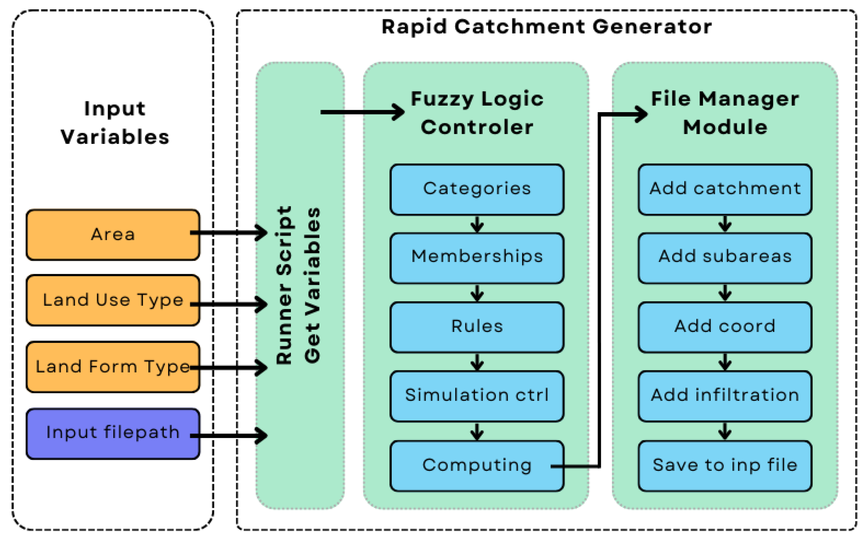
Despite significant advances in automated SWMM construction and parameter optimization, a critical gap remains in translating qualitative catchment descriptions into quantitative model parameters rapidly and accessibly. Existing tools either require extensive GIS data preprocessing, demand specialized expertise for calibration, or produce oversimplified models unsuitable for detailed analysis. While fuzzy logic has demonstrated promise in hydrological applications, its integration into mainstream urban drainage modeling workflows—particularly for SWMM catchment parameterization—remains largely unexplored. This paper addresses these limitations by presenting the RCG, a novel fuzzy logic-based tool that bridges the gap between expert hydrological knowledge and model parameterization. Unlike existing approaches that focus on either full automation with complex data requirements or simplified calculators with limited functionality, RCG enables practitioners to generate SWMM-ready catchment parameters from minimal qualitative inputs (area, landform type, and land cover type) within seconds. By codifying hydrological expertise into fuzzy rules and directly integrating with SWMM input files, this research demonstrates how fuzzy inference systems can transform the catchment modeling workflow—reducing setup time by orders of magnitude while maintaining the flexibility for subsequent detailed calibration. This approach not only democratizes access to advanced stormwater modeling but also provides a reproducible framework for rapid scenario testing essential for climate-resilient urban drainage design.

2. Materials and Methods

2.1. Storm Water Management Model and Subcatchment Parameters

SWMM is a dynamic rainfall–runoff simulator widely used for single-event and continuous modeling of urban drainage systems [27,28,29,30,31]. Its modular code executes five principal tasks: CORE (data management, simulation control, and reporting), RUNOFF (surface hydrology), FLOW & WATER QUALITY (hydraulic routing and pollutant transport), HEADER FILES (global definitions), and MISCELLANEOUS FUNCTIONS (time, numerics, and geometry) [32]. In the RUNOFF module, each rectangular subcatchment is treated as a non-linear reservoir; sheet-flow discharge Q (m³ s⁻¹) is estimated by Equation (1):

$$\mathrm{Q}=\mathrm{W}{\displaystyle \frac{{\left(\mathrm{h}-{\mathrm{h}}_{\mathrm{p}}\right)}^{5/3}}{{\mathrm{n}}_{\mathrm{p}}}}{\mathrm{i}}_{\mathrm{p}}^{1/2}$$

(1)

where W = hydraulic width (m), h = precipitation depth (m), h_p = depression storage depth (m), n_p = composite Manning’s roughness coefficient (s·m⁻¹/³), and i_p = average slope (-).

Infiltration is evaluated with one of four embedded methods—Horton, Green–Ampt, modified Horton, or incremental SCS curve number—each relating infiltration capacity to antecedent moisture through empirically or physically based equations [33,34,35,36]. All remaining hydrological processes (evaporation, groundwater exchange, LID controls) employ SWMM’s standard formulations and are held constant in this study to isolate the influence of subcatchment parameters on runoff generation.

A modeled area is divided into drainage basins bounded by watershed divides and drained toward a single outfall. For hydraulic consistency, SWMM represents each subcatchment as an idealized rectangle of uniform slope; its geometric and hydraulic descriptors are summarized in

Table 1. SWMM subcatchment characteristic features.

Feature Name	Unit	Description
Area	ha	Area of the subcatchment, including any LID controls.
Width	m	Characteristic width of the overland flow path for sheet flow runoff.
Slope	%	Average percent slope of the subcatchment.
Imperv	%	Percent of the land area (not including any LIDs) that is impervious.
N-Imperv	-	Manning’s n for overland flow over the impervious portion of the subcatchment.
N-Perv	-	Manning’s n for overland flow over the previous portion of the subcatchment.
Dstore-Imperv	m	Depth of depression storage on the impervious portion of the subcatchment.
Dstore-Perv	m	Depth of depression storage on the previous portion of the subcatchment.
% Zero-Imperv	%	Percent of the impervious area with no depression storage.
Infiltration Data	-	Infiltration models (Horton, Modified Horton, Green–Ampt, Modified Green–Ampt, and Curve Number (SCS)).

. The present work varies only hydraulic width, slope, and impervious fraction—identified in Section 2.4 as the dominant controls on both runoff and infiltration—while all other parameters follow the default or literature-recommended values listed in the software manual [9].

2.2. Fuzzy Logic

Dr. Lotfi Zadeh first introduced the term “fuzzy logic” in the 1960s, defining a framework for handling vague, uncertain, or unclear information [37]. Fuzzy sets explicitly model the relationship between vague linguistic descriptors used to describe the “state” of a component and the resulting score assigned to that component. This process, known as “fuzzification”, takes values (e.g., scores) and classifies them into an arbitrary number of categories or sets (e.g., “low” or “high”) [38]. The value in the reference set is called the degree of membership [39]. The degree of membership of an element in a fuzzy set ranges from 0 to 1, inclusive. Unlike ordinary sets, which have “hard” boundaries, the boundaries of fuzzy sets are “soft”, reflecting the uncertainty in the boundaries of the set. This means that a result can belong to more than one set [38]. Thus, fuzzy logic provides the concept of an intermediate value between 0 and 1. Intermediate values are partly true and partly false [40].

Fuzzy logic has several well-known advantages: it is flexible, based on natural language, and fundamentally simple [41]. Additionally, the model can be constructed using expert knowledge and is resistant to ambiguous or imprecise data [42]. In fuzzy systems, mapping the input data is essential to obtain results based on them [43]. The elements of the fuzzy set (Ã) in Mamdani’s fuzzy inference method satisfy the continuity of membership property [44], so the following should be considered (2):

$$Ã=\{(\mathrm{x}, {\mathsf{\mu }}_{\mathrm{Ã}}(\mathrm{x})) | \mathrm{x}\in \mathrm{X}\}$$

(2)

where à is a fuzzy set in the space X, x is an element or member of the set, and ${\mathsf{\mu }}_{\mathrm{Ã}}$(x) the membership class of element x in the fuzzy set à with the condition ${\mathsf{\mu }}_{\mathrm{Ã}}$: X → [0, 1]. In the design of fuzzy controllers, the triangular membership function (MF) is one of the most extensively used and accepted. It defines a triangular membership area that extends from point a to point c and has a peak at point b. The value of membership equals 0 for x ≤ a and x ≥ c and increases linearly from a to b and from b to c. It can be represented and calculated according to Equation (3):

$${\mathsf{\mu }}_{\mathrm{t}\mathrm{r}\mathrm{i}\mathrm{m}\mathrm{f}}\left(\mathrm{x};\mathrm{a},\mathrm{b},\mathrm{c}\right)=\mathrm{m}\mathrm{a}\mathrm{x}\left(\mathrm{m}\mathrm{i}\mathrm{n}\left({\displaystyle \frac{\mathrm{x}-\mathrm{a}}{\mathrm{b}-\mathrm{a}}},{\displaystyle \frac{\mathrm{c}-\mathrm{x}}{\mathrm{c}-\mathrm{b}}},0\right)\right)$$

(3)

The aggregated fuzzy outputs must be converted into crisp values through defuzzification to enable hydrological interpretation. This study employs the centroid method (Equation (4)), which calculates the geometric center of the aggregated membership function to preserve gradient-driven runoff dynamics:

$${\mathrm{x}}_{\mathrm{output}}={\displaystyle \frac{{\int }_{\mathrm{a}}^{\mathrm{c}}\mathrm{x}\cdot {\mathsf{\mu }}_{\mathrm{out}}\left(\mathrm{x}\right)\mathrm{d}\mathrm{x}}{{\int }_{\mathrm{a}}^{\mathrm{c}}{\mathsf{\mu }}_{\mathrm{out}}\left(\mathrm{x}\right)\mathrm{d}\mathrm{x}}}$$

(4)

where:

• ${\mathsf{\mu }}_{\mathrm{out}}\left(\mathrm{x}\right)$: Aggregated membership function from fuzzy rule evaluation (dimensionless);

• [a, c]: Domain of the output variable (e.g., imperviousness range 0–100%);
• x: Crisp output value used in SWMM parameterization (e.g., slope).

The centroid method avoids artificial thresholds between land cover classes, crucial for modeling transitional zones.

2.3. Least Absolute Shrinkage and Selection Operator with Cross-Validation

Introduced by Tibshirani [45], the Least Absolute Shrinkage and Selection Operator with Cross-Validation (LassoCV) model has become a cornerstone algorithm in regularized linear regression. This model is defined by the following cost function (5):

$$\begin{array}{c}\mathrm{m}\mathrm{i}\mathrm{n}\\ \mathsf{\beta }\end{array}\left({\displaystyle \frac{1}{2\mathrm{n}}}||\mathrm{X}\mathsf{\beta }-\mathrm{y}{||}_2^2+\propto ||\mathsf{\beta }{||}_1\right)$$

(5)

where X is the feature matrix, y is the response vector, β is the coefficient vector, α is this regularization parameter, and n is the number of samples. In this equation, $||\mathrm{X}\mathsf{\beta }-\mathrm{y}{||}_2^2$ represents the L2 norm, also known as the Euclidean norm, which measures the sum of the squared differences between the predicted and actual values (6):

$$||\mathrm{X}\mathsf{\beta }-\mathrm{y}{||}_2^2=\sum _{\mathrm{i}=0}^{\mathrm{n}}{\left(\mathrm{X}\mathsf{\beta }-{\mathrm{y}}_{\mathrm{i}}\right)}^2$$

(6)

The term ${||\mathsf{\beta }||}_1$ denotes the L1 norm, also known as the Manhattan norm, which measures the sum of the absolute values of the coefficients (7):

$${||\mathsf{\beta }||}_1=\sum _{\mathrm{i}=0}^{\mathrm{n}}{\left(\mathrm{X}\mathsf{\beta }-{\mathrm{y}}_{\mathrm{i}}\right)}^2$$

(7)

The value of α is automatically selected through cross-validation [45]. The algorithm employs L1 regularization, which tends to zero out coefficients for less significant variables. This is particularly useful in scenarios with a high number of collinear variables. In Python, the LassoCV function is available in the scikit-learn library and automatically performs cross-validation to find the optimal α parameter [46]. In practice, LassoCV is frequently employed in high-dimensional data analysis where variable selection is key. It is robust to noise and can be used in situations where the data are incomplete or contain many variables that are correlated with each other [47].

2.4. Feature Selection

To identify the most influential catchment features for rapid prototyping, simulations were conducted in SWMM 5.2.2 using a 1-hectare urban catchment subjected to a synthetic Euler-type rainfall event (3-year return period, 120 min in duration, peak intensity of 102 mm/h). The 24-h simulation employed Kinematic Wave routing and the Horton infiltration model (max rate = 75 mm/h, min rate = 10 mm/h, decay constant = 4 h⁻¹) to isolate natural hydrological processes without LID interventions.

A full factorial design tested 116,640 parameter combinations (

Table 2. Ranges of simulated data.

Subcatchment Feature	Unit	Values
Width	m	[1, 5, 10, 25, 50, 75, 100, 125, 150]
Slope	%	[0.1, 1, 2, 3, 4, 5, 6, 7, 8, 9]
PercImperv	%	[1, 20, 40, 60, 80, 100]
N-Imperv	-	[0.011, 0.015]
N-Perv	-	[0.13, 0.40, 0.80]
D-Imperv	mm	[1.27, 2.54]
D-Perv	mm	[2.54, 5.08, 7.62]
PctZero	%	[1, 20, 40, 60, 80, 100]

) using PySWMM 1.2.0 for automated input/output management. Parameter ranges were constrained to realistic urban scenarios: widths (1–150 m) representing overland flow paths in depressions or engineered features such as roadways; slopes (0.1–9%) categorized as “little/no slope” (0–3%) and “gentle slopes” (4–9%) per USDA [48] standards; imperviousness (1–100%) spanning green spaces to fully paved areas; and depression storage values reflecting material-specific properties (1.27 mm for smooth asphalt to 7.62 mm for vegetated litter). Manning’s coefficients and zero-depression percentages were limited to ranges typical of urban drainage manuals to reduce calibration complexity.

This exploration enabled prioritization of parameters with the greatest hydrological impact, forming the basis for the RCG’s simplified input requirements while maintaining physical realism. The data-driven methodology complements the theoretical framework of SWMM’s runoff equation (Equation (1)), offering an independent pathway to identify dominant catchment features. Critically, this approach circumvents potential SWMM implementation artifacts, such as numerical instabilities from floating-point precision limitations, ensuring robust parameter sensitivity conclusions.

Based on the calculation reports, it is concluded that the parameters “Width”, “Slope”, and “Impervious” are strongly positively correlated with “Total Runoff”. A weak negative correlation was observed for the features “N-Imperv”, “N-Perv”, “Dstore-Imperv”, and “Dstore-Perv”. Confirmation is provided by the results of the calculated variable weights of the linear regression model (Figure 1). The importance of the features was determined using the LascoCV model. According to this model, the parameters “Width” and “Slope” have the greatest influence on the value of “Total Runoff” (Figure 2).

A negative correlation with infiltration is observed for the parameters “Imperviousness”, “Width”, and “Slope”. A weak positive correlation was observed with the parameter “N-Perv”. The feature weights calculated for the linear regression model (Figure 3) confirm the observed correlations. The feature importance determined using the LassoCV model shows that “Width”, “Slope”, and “Imperviousness” have the greatest impact on infiltration.

The correlation patterns obtained in Figure 1, Figure 2, Figure 3 and Figure 4 mirror findings reported in earlier SWMM studies. Numerous authors show that steeper ground slopes accelerate overland flow and therefore increase runoff velocities [49], while a higher share of impervious surfaces consistently raises both peak discharge and total runoff volume [50,51]. Although discussed less frequently, hydraulic width—or, conversely, flow length—also modulates hydrograph shape: work translated to SWMM geometry indicates that widening the overland path leads to a systematic rise in peak flow under kinematic-wave routing [34,52].

Both our linear regression and LassoCV models capture the same hierarchy of influence, even though regularization in Lasso suppresses the weight of variables correlated with others. Width, Slope, and Imperviousness remain the dominant predictors of runoff and infiltration. Thus, converging evidence from the literature and our data-driven sensitivity study confirms that these three descriptors are sufficient for rapid prototyping of catchments and form a robust basis for the fuzzy-logic rules implemented in the Rapid Catchment Generator.

2.5. Rapid Catchment Generator

The Rapid Catchment Generator (RCG) creates a new SWMM subcatchment from three descriptors—area, landform type, and land cover type—without any manual editing of the .inp file. After a user supplies the values, a runner script passes them to a fuzzy logic controller, which converts the descriptors into hydraulic width, average slope, and impervious fraction (Figure 5). These crisp parameters are then forwarded to a file manager module, which writes the corresponding [SUBCATCHMENTS], [SUBAREAS], [COORDINATES], and [INFILTRATION] sections and saves the updated file. When the write operation is complete, the script prompts for the next set of inputs, so multiple catchments can be generated in sequence. The workflow is fully object-oriented, written in Python 3, and reduces model-setup time from hours to seconds while keeping the rule base transparent and easy to adapt.

To build the catchment generator, landform types were classified according to

Table 3. Fuzzy logic classification of landform–slope relationships with parameter ranges and global system alignment [48,52,53].

Classification	Scoring Range (%)	Fuzzy Parameters Trimf (a, b, c)	Alignment with Global Systems
Lowlands	0–1	(0, 0, 1)	USDA “Nearly Level”; USGS “Flat to gentle slopes”; Meybeck et al. [53] “Plains”
Flats and plateaus	0–2.5	(0, 1, 2.5)	USDA “Nearly Level”; USGS “Flat to gentle slopes”; Meybeck et al. [53] “Lowlands and Platforms”
Flats and plateaus in combination with hills	1–5	(1, 2.5, 5)	USDA “Gently Sloping”; USGS “Flat to gentle slopes”; Meybeck et al. [53] “Mid-Altitude Plains”
Hills with gentle slopes	2.5–8	(2.5, 5, 8)	USDA “Gently Sloping”; USGS “Gentle to moderate slopes”; Meybeck et al. [53] “Rugged Lowlands & Hills”
Steeper hills and foothills	5–8	(5, 8, 15)	USDA” Strongly Sloping”; USGS “Gentle to moderate slopes”; Meybeck et al. [53] “Mid Altitude Plateaus”
Hills and outcrops of mountain ranges	8–20	(8, 15, 20)	USDA “Moderately Steep”; USGS “Gentle to moderate slopes”; Meybeck et al. [53] “High Altitude Plateaus”
Higher hills	15–30	(15, 20, 30)	USDA “Steep”; USGS “Moderate slopes”; Meybeck et al. [53] “Hills”
Mountains	20–40	(20, 30, 40)	USDA “Very Steep”; USGS “Step slopes”; Meybeck et al. [53] “Mid Altitude Mountains”
Highest mountains	30–60	(30, 50, 60)	USDA “Extremely Steep”; USGS “Very step”; Meybeck et al. [53] “Very High Altitude Mountains”

and land cover types according to

Table 4. Fuzzy logic classification of impervious surface characteristics with parameter ranges and global system alignment [56,57,58,59].

Classification	Scoring Range (%)	Fuzzy Parameters Trimf (a, b, c)	Alignment with Global Systems
Marshes	0–2	(0, 0, 2)	EPA ROE “Emergent Herbaceous Wetlands”; NLCD 95 “Emergent Herbaceous Wetlands”; Łachowski, [58] “Very low”; CLC 411 “Inland Marshes”
Arable	0–4	(0, 2, 4)	EPA ROE “Cultivated Crops”; NLCD 82 “Cultivated Crops”; Łachowski, [58] “Very low”; CLC 21x “Arable Land”
Meadows	2–8	(2, 5, 8)	EPA ROE “Grassland/Herbaceous”; NLCD 71 “Grassland/Herbaceous”; Łachowski, [58] “Very low”; CLC 231 “Pastures” or CLC 321 “Natural Grasslands”
Forests	5–9	(5, 7, 9)	EPA ROE “Forest”; NLCD 41–43 „Forests”; Łachowski, [58] “Very low”; CLC 311–313 “Forests”
Rural	7–15	(7, 11, 15)	EPA ROE “Pasture/Hay”; NLCD 81 “Pasture/Hay”; Łachowski, [58] “Low”; CLC 231 “Pastures”
Vegetated mountains	5–25	(5, 15, 25)	EPA ROE “Shrub/Scrub”; NLCD 52 “Shrub/Scrub”; Łachowski, [58] “Low”; CLC 322 “Moors and Heathland” or CLC 324 “Transitional Woodland-Shrub”
Rocky mountains	20–60	(20, 30, 60)	EPA ROE “Barren”; NLCD 31 “Barren Land”; CLC 333 “Sparsely Vegetated Areas”
Suburban (low imperviousness)	10–40	(10, 25, 40)	EPA ROE “Developed, Low Intensity”; NLCD 22 “Developed, Low Intensity”; Łachowski, [58] “Low”; CLC 112 “Discontinuous Urban Fabric”
Suburban (high imperviousness)	35–65	(35, 50, 65)	EPA ROE “Developed, Low Intensity”; NLCD 22 “Developed, Low Intensity”; Łachowski, [58] “Medium”; CLC 112 “Discontinuous Urban Fabric”
Urban (low imperviousness)	30–60	(30, 45, 60)	EPA ROE “Developed, Medium Intensity”; NLCD 23 “Developed, Medium Intensity”; Łachowski, [58] “Medium”; CLC 112 “Discontinuous Urban Fabric”
Urban (medium imperviousness)	50–80	(50, 65, 80)	EPA ROE “Developed, Medium Intensity”; NLCD 23 “Developed, Medium Intensity”; Łachowski, [58] “High”; CLC 112 “Discontinuous Urban Fabric”
Urban (high imperviousness)	75–100	(75, 85, 100)	EPA ROE “Developed, High Intensity”; NLCD 24 “Developed, High Intensity”; Łachowski, [58] “High”; CLC 111 “Continuous Urban Fabric”

. The landform variable encapsulates geomorphological characteristics relevant to hydrological processes, including slope-driven runoff dynamics, erosion potential, and water retention capacity. Developed through a synthesis of USDA slope classes [48], USGS terrain categories [52], and Meybeck geomorphological typology [53], the classification in Table 3 integrates anthropogenic features from urban hydrology studies [54,55]. Modifications ensure fuzzy logic compatibility: (1) intentionally overlapping slope ranges eliminate abrupt transitions between categories, enabling smooth centroid defuzzification; and (2) hybrid terrain descriptors (e.g., “Flats/Plateaus + Hills”) bridge natural and urbanized landscapes. This adaptation preserves alignment with global systems while addressing the gradient-driven complexities of anthropogenic catchments.

Category-specific definitions:

• Lowlands (0–1%): Combines nearly level terrain with wetland saturation thresholds; use for swamps, peat bogs, or floodplains with stagnant surface flow.
• Flats and Plateaus (0–2.5%): Urban grids and industrial zones. Apply to areas requiring minimal grading for storm sewer placement (e.g., downtown cores).
• Flats/Plateaus + Hills (1–5%): Hybrid of gentle slopes and undulating terrain. Ideal for residential neighborhoods where gentle slopes allow gravity-fed drainage without erosion risks.
• Hills with Gentle Slopes (2.5–8%): Extends gently sloping terrain with urban suitability criteria; use for developed hillsides (e.g., residential zones) with moderate erosion risk.
• Steeper Hills and Foothills (5–8%): Aligns with landslide risk thresholds; apply to convex slopes with concentrated runoff (e.g., gully-prone areas, natural reserves).
• Hills/Mountain Outcrops (8–20%): Merges hilly and moderately sloping terrain ranges; use for foothills with mixed forest-agro-tourism land use.
• Higher Hills (15–30%): Integrates strongly sloping terrain with sediment transport thresholds; suitable for terraced agriculture or logging areas requiring debris flow controls.
• Mountains (20–40%): Combines mountainous and steep terrain classes; apply to snowmelt-dominated alpine catchments or ski resort watersheds.
• Highest Mountains (30–60%): Extends extreme slope systems; reserved for slopes with rockfall hazards or glacial headwaters.

The impervious surface classification presented in Table 4 utilizes fuzzy logic principles to systematically categorize land cover types according to their imperviousness percentages, ensuring compatibility with global classification frameworks [56,57,58,59,60]. Overlapping fuzzy membership functions were deliberately designed to capture the inherent variability and transitional nature of urban and suburban landscapes. Through centroid defuzzification, the classification resolves potential ambiguities between adjacent imperviousness categories. The parameter ranges were calibrated based on empirical data from international and regional sources, ensuring their relevance and accuracy for Central European land cover analyses.

Category-specific definitions:

• Marshes (0–2%): Natural runoff buffers in urban wetlands or floodplain parks. Use for designated retention zones within city limits.
• Arable (0–4%): Urban farms or peri-urban croplands. Apply to community gardens or temporary greenfields during development phases.
• Meadows (2–8%): Managed turf in parks, golf courses, or roadside verges. Suitable for recreational grasslands with irrigation systems.
• Forests (5–9%): Urban woodlots with compacted trails. Use for municipal parks where tree cover coexists with paved pathways.
• Rural (7–15%): Urban fringe villages transitioning to suburbs. Apply to areas with farmstead conversions or unpaved service roads.
• Vegetated Mountains (5–25%): Engineered slopes in city parks or green belts. Use for terraced hillsides with drainage controls.
• Rocky Mountains (20–60%): Quarries or bedrock outcrops in urban expansion zones. Apply to natural terrain preserved within developments.
• Suburban Low Imperviousness (10–40%): Standard single-family residential areas. Ideal for neighborhoods with mandatory green space ratios.
• Suburban High Imperviousness (35–65%): Townhouse districts or low-rise apartments. Use for areas with shared amenities (playgrounds, parking courts).
• Urban Low Imperviousness (30–60%): Green infrastructure showcase zones. Apply to streetscapes with bioswales or permeable pedestrian areas.
• Urban Medium Imperviousness (50–80%): Commercial corridors. Suitable for strip malls with required stormwater planters.
• Urban High Imperviousness (75–100%): Downtown cores. Use for high-rises with mandatory retention vaults or rooftop detention.

The fuzzy logic controller was designed using rule sets that integrate all variable combinations from Table 3 and Table 4, with hydrological outcomes systematically quantified across inference classes. Slope and permeability categories, along with their corresponding triangular membership function parameters (a, b, c), are detailed in Table 3 (slope classifications) and Table 4 (permeability ranges). Model behavior is further visualized through response surfaces for slope (Figure 6) and imperviousness (Figure 7), illustrating how input variations influence hydrological predictions. To optimize performance, hydrologists conducted an expert-led calibration process using Storm Water Management Model (SWMM) test catchments. This iterative refinement adjusted both membership function parameters and controller rules, ensuring alignment with empirical hydrological dynamics. The integration of theoretical frameworks and data-driven validation enhances the system’s reliability in replicating real-world water management scenarios.

The data from the input file being processed are converted to a data frame using the Pandas package in Python.

Table 5. Method of data generation.

Parameter Name	Explanation
Name	Catchment names (IDs) are generated by adding a number as a suffix.
Rain gage	When a “Rain Gage” exists in the uploaded file, it will be assigned to the catchment being built. Where it does not exist, it will be added to the file along with the “time series” and assigned to the catchment area being generated.
Outlet	If there are outlets in the passed file, the system will automatically assign the first one to the catchment; if there are not, the name of the generated catchment area will be assigned.
Area	A parameter passed by the user.
Percent Imperv	The parameter is calculated by the fuzzy logic module and assigned to the catchment.
Width *	In the generated model, catchments are represented as equivalent rectangles to account for natural elongation. The width of the flow path Lw in the Kinematic Wave (KW) model is derived from the catchment area A and a compactness-adjusted flow length Lflow. The flow length is defined as $L_{flow}=A·\mathrm{10,000}·C$ where A is the catchment area in hectares (converted to m2) and C is the compactness $(\mathrm{C}\sqrt{2}$, typically 1.5–2.0 for irregular or elongated catchments). The flow path width Lw is then calculated as $L_W={\displaystyle \frac{A·\mathrm{10,000}}{L_{flow}}}$.
Percent Slope	The parameter is calculated by the fuzzy logic module and assigned to the catchment.
N-Imperv	The value taken was based on the linguistic variables passed to the fuzzy logic controller, which were previously mapped with Manning coefficients.
N-Perv
Dstore-Imperv	Values are taken from the linguistic variables passed to the fuzzy logic controller, which have previously been mapped with Manning coefficients.
Dstore-Perv
% Zero-Imperv
RouteTo	Runoff from impervious and pervious areas flows directly to the outlet.
Coordinate	Square-shaped catchments are generated, located so that one side is the edge of the contact.

Note: * Explanation based on the methodology described in [61].

shows the characteristic catchment parameters in SWMM and an explanation of how they are generated.

3. Results

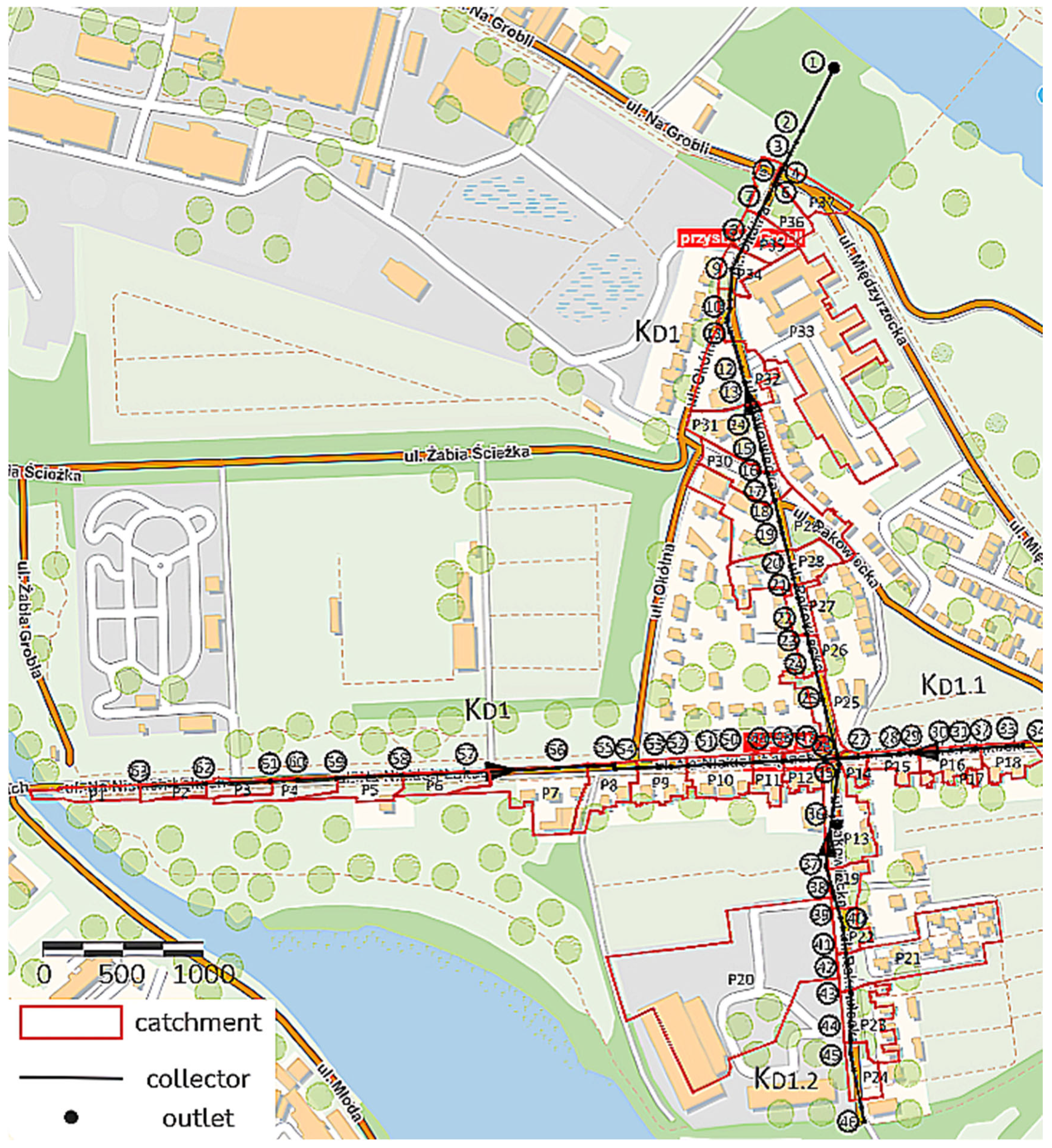
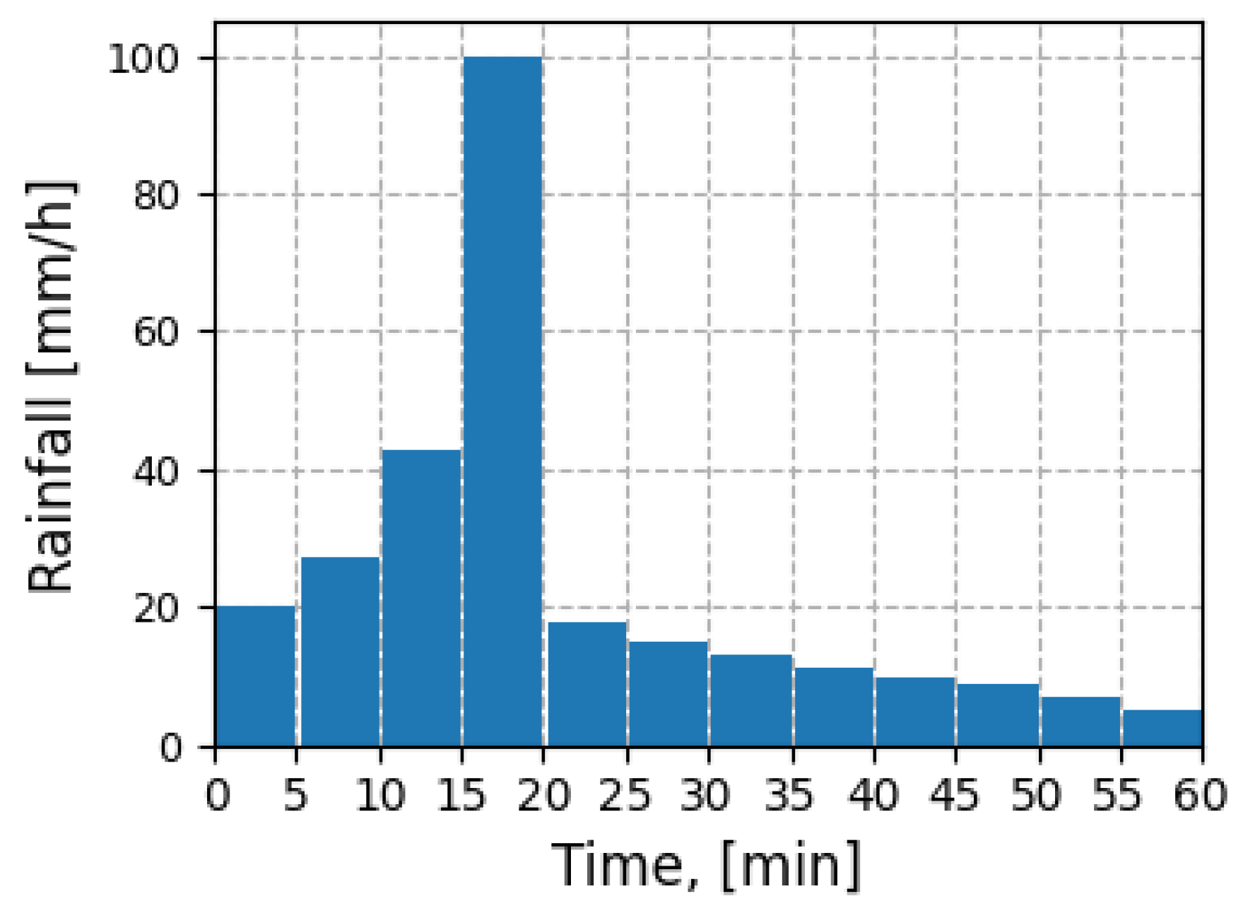
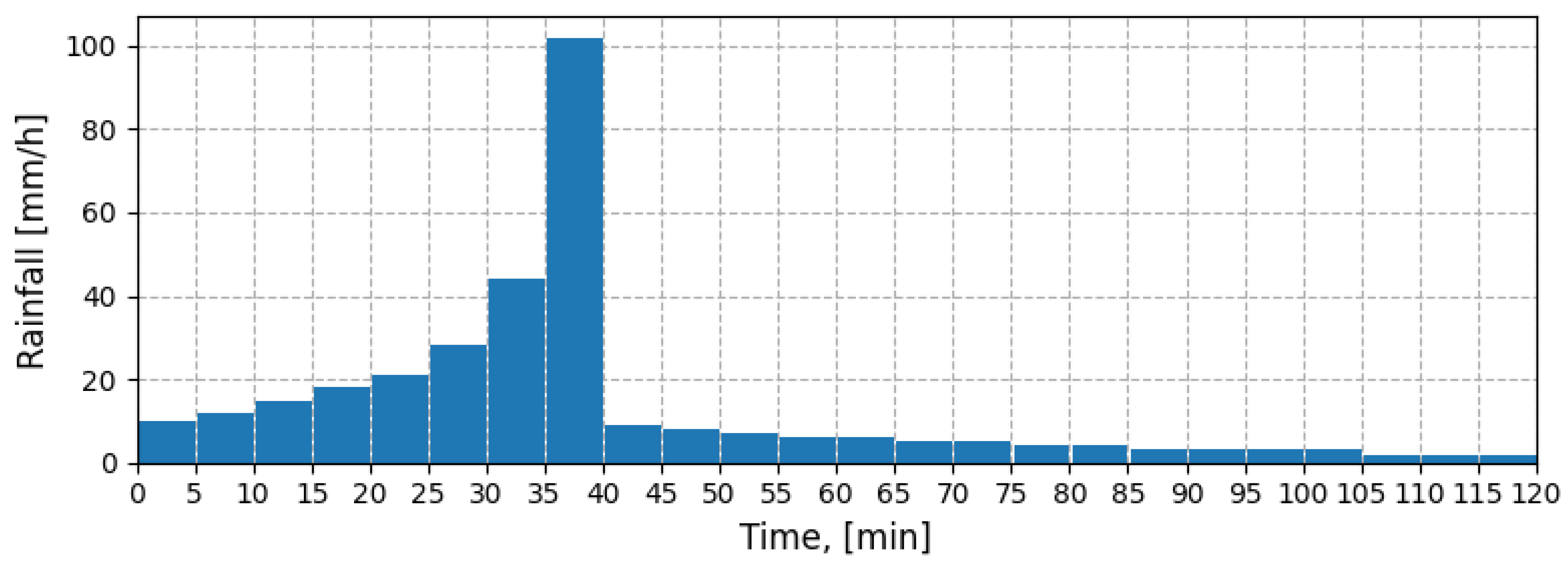
To evaluate the performance of RCG 0.1.0, the test and generated catchments were compared. The test catchment, located in the Rakowiec Estate in Wrocław, Poland, covers approximately 10 hectares and features a mix of residential, commercial, and green spaces (Figure 8). Bordered by the Odra and Oława Rivers, its drainage system discharges into the Odra River. Divided into 37 subcatchments (P1–P37), the test area reflects the diversity of land cover and topography within the estate. The simulation used two rainfall events based on the Euler II model, each with a three-year recurrence interval. The first event had a peak intensity of 102 mm/h and lasted 60 min (Figure 9), while the second had a peak intensity of 102 mm/h and lasted 120 min (Figure 10). These rainfall events represent real-world conditions that could significantly impact the drainage system’s capacity [28].

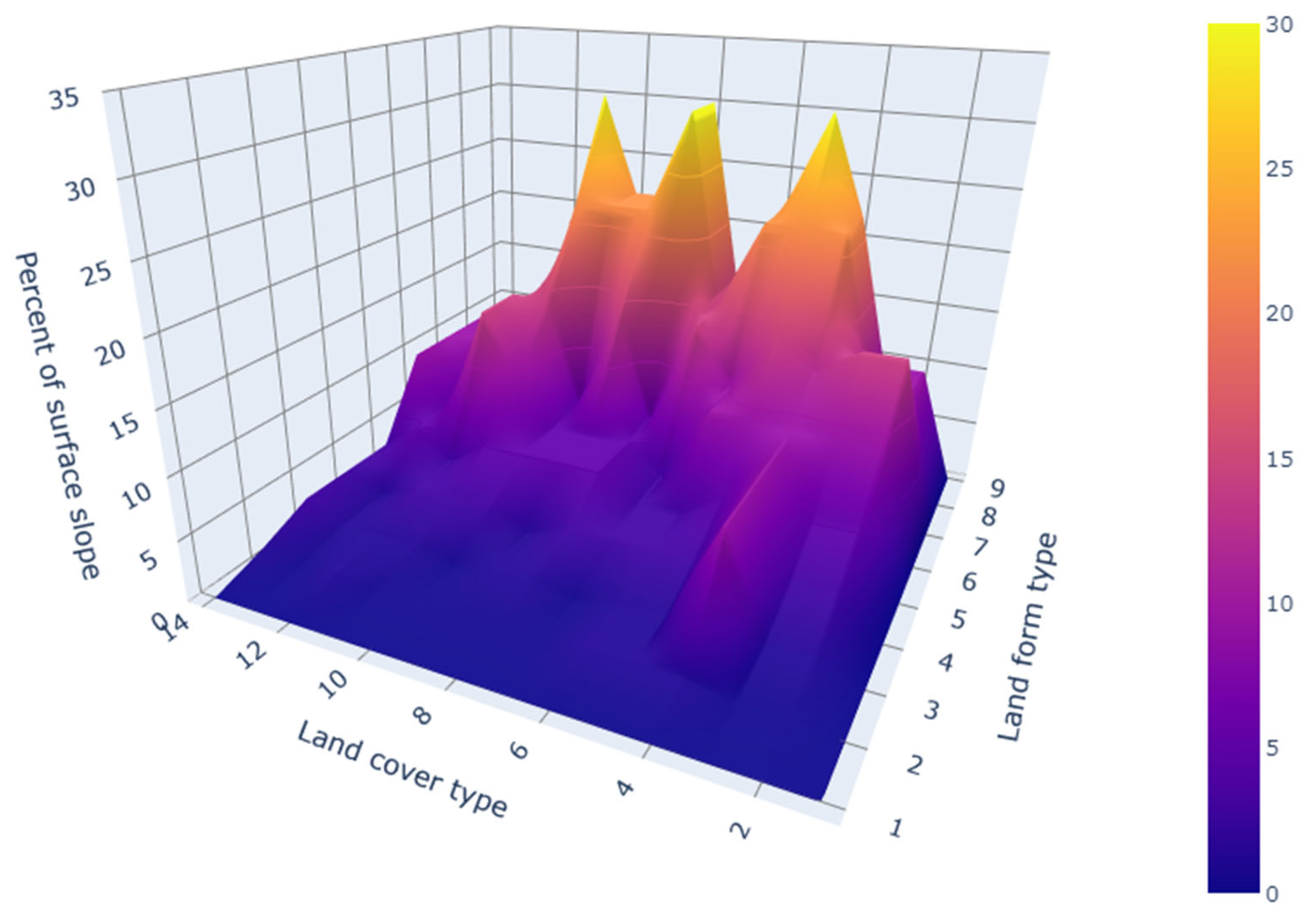
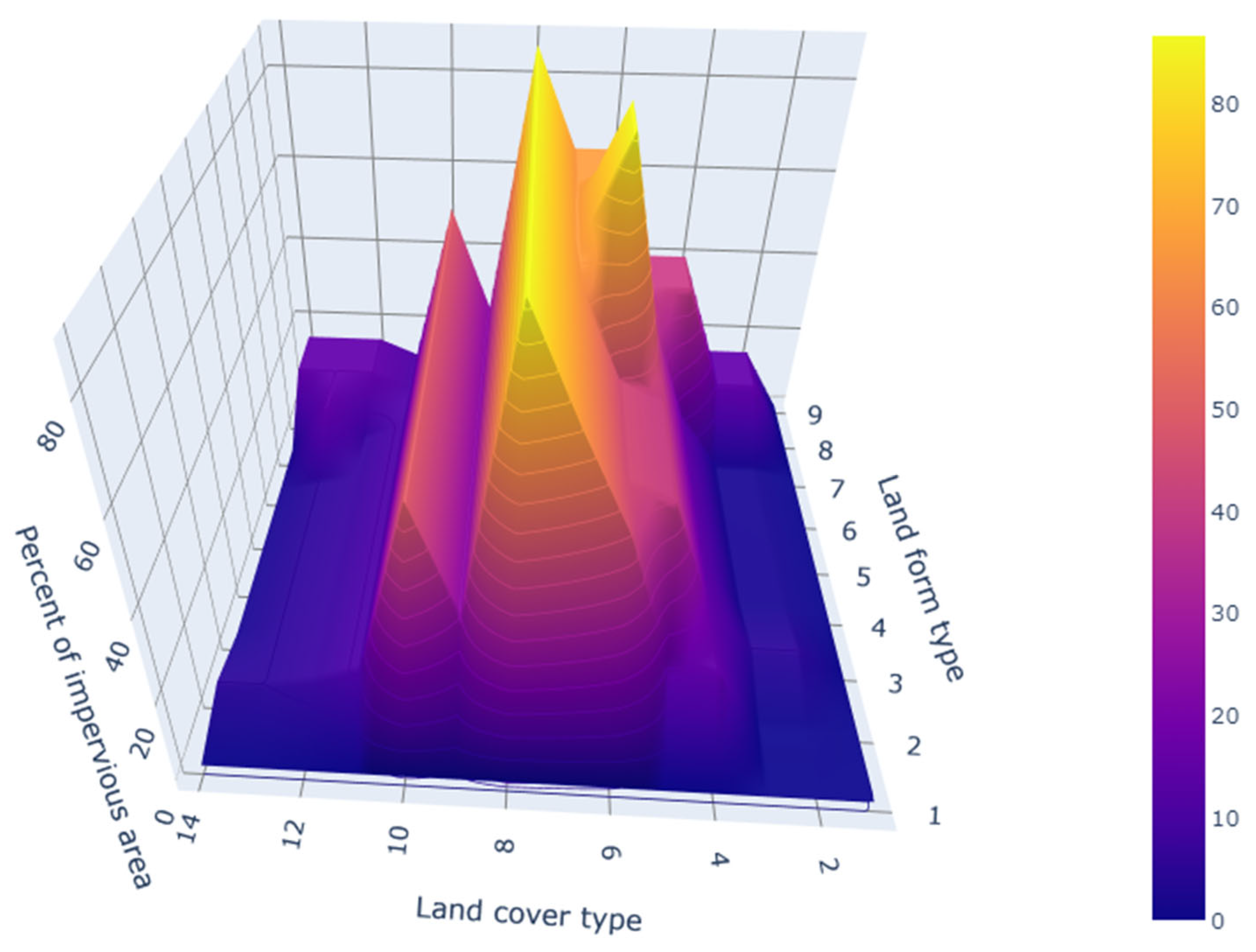
The RCG utilizes linguistic variables to define catchment characteristics, which influence hydrological behavior.

Table 6. Input variables used to reproduce the test catchment.

Name	Landform Type	Land Cover Type
G2, G3, G4, G5, G6, G8, G13, G19, G20, G27, G28, G29, G37	flats and plateaus	urban, weakly impervious
G1, G7, G9, G10, G11, G12, G18, G21, G22, G23, G26, G32, G34, G35, G36	flats and plateaus	urban, moderately impervious
G14, G15, G16, G17, G25, G33	flats and plateaus	urban, highly impervious
G24, G30, G31	flats and plateaus	suburban, weakly impervious

outlines the land use and landform categories assigned during the generation process. To replicate the test subcatchments using the RCG, each catchment labeled ‘Pn’ was paired with a generated equivalent, labeled ‘Gn’ (

Table 7. Summary of areas and hydrologic responses (runoff and infiltration) for test (P) and generated (G) subcatchments during 60- and 120-min Euler II rainfall events.

Name	Area [ha]	Precipitation Euler II 60 min				Precipitation Euler II 120 min
		Runoff [m3]		Infiltration [m3]		Runoff [m3]		Infiltration [m3]
		Test	Gen	Test	Gen	Test	Gen	Test	Gen
P1–G1	0.1158	16.1	17.3	10.0	9.4	18.7	20.0	11.6	10.9
P2–G2	0.0821	9.7	8.5	8.9	10.5	11.3	9.8	10.3	12.1
P3–G3	0.0885	11.8	9.1	8.2	11.3	13.7	10.6	9.5	13.1
P4–G4	0.1355	12.8	14.0	18.1	17.3	14.9	16.2	20.9	20.0
P5–G5	0.1597	19.5	16.5	16.6	20.4	22.7	19.1	19.2	23.6
P6–G6	0.1449	15.2	14.9	17.7	18.5	17.7	17.4	20.5	21.4
P7–G7	0.3857	50.0	57.4	37.1	31.3	58.1	66.5	43.0	36.2
P8–G8	0.2053	21.6	21.2	24.9	26.2	25.1	24.6	28.9	30.3
P9–G9	0.1801	22.8	26.8	17.9	14.6	26.5	31.1	20.8	16.9
P10–G10	0.2117	28.5	31.5	19.3	17.2	33.2	36.6	22.3	19.9
P11–G11	0.1144	15.4	17.0	10.4	9.3	18.0	19.8	12.0	10.8
P12–G12	0.1331	21.9	19.8	8.0	10.8	25.4	23.0	9.2	12.5
P13–G13	0.1361	29.9	32.1	39.1	39.7	34.9	37.3	45.2	46.0
P14–G14	0.2406	8.6	11.6	4.3	1.9	10.1	13.6	5.0	2.1
P15–G15	0.6267	16.9	22.2	7.7	3.5	19.8	26.0	8.9	4.1
P16–G16	0.0982	20.6	27.6	10.1	4.4	24.1	32.4	11.7	5.1
P17–G17	1.9574	2.9	2.8	0.4	0.4	3.4	3.3	0.5	0.5
P18–G18	0.1118	19.1	21.3	11.9	11.6	22.4	24.8	13.8	13.5
P19–G19	0.3114	10.1	11.5	14.8	14.3	11.8	13.4	17.1	16.5
P20–G20	0.1432	11.5	10.1	10.7	12.5	13.4	11.8	12.4	14.5
P21–G21	0.0142	84.1	93.1	54.2	50.8	97.8	107.8	62.8	58.9
P22–G22	0.1422	220.5	288.9	212.4	158.7	256.4	334.6	246.0	183.8
P23–G23	0.1143	31.5	35.8	22.7	19.5	36.7	41.6	26.3	22.6
P24–G24	0.0598	7.6	7.7	23.6	23.7	8.8	9.0	27.4	27.4
P25–G25	0.1556	27.3	30.2	5.6	4.8	32.0	35.4	6.5	5.6
P26–G26	0.0747	10.8	11.1	5.4	6.1	12.6	12.9	6.2	7.0
P27–G27	0.0988	12.6	10.2	8.9	12.6	14.7	11.8	10.4	14.6
P28–G28	0.3196	35.3	33.0	35.0	40.7	41.2	38.3	40.6	47.2
P29–G29	0.5846	70.0	60.3	57.8	74.5	81.8	69.9	66.9	86.3
P30–G30	0.2087	18.2	11.9	28.2	36.3	21.2	13.8	32.7	42.0
P31–G31	0.2962	29.7	16.8	35.8	51.5	34.7	19.6	41.4	59.6
P32–G32	0.3639	55.2	54.1	23.1	29.5	64.5	62.8	26.8	34.2
P33–G33	1.4477	231.6	280.4	55.3	44.7	271.9	326.3	64.1	51.7
P34–G34	0.1167	15.7	17.4	9.7	9.5	18.4	20.2	11.2	11.0
P35–G35	0.1684	20.3	25.1	16.5	13.7	23.8	29.1	19.1	15.8
P36–G36	0.2098	21.4	31.3	24.9	17.0	25.0	36.2	28.8	19.7
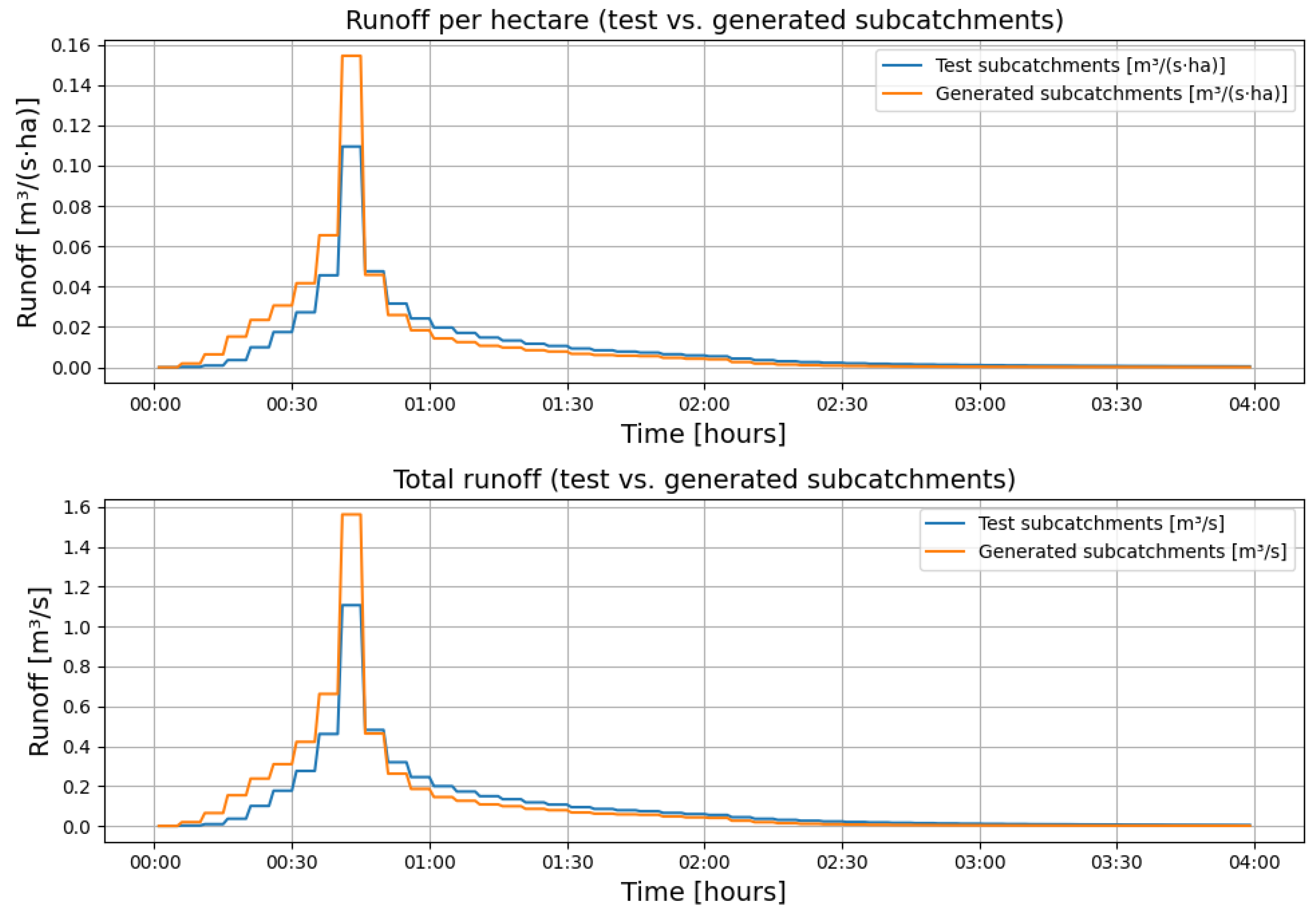
P37–G37	0.1553	14.6	16.0	19.7	19.8	17.1	18.6	22.8	22.9

). Runoff hydrographs for the 60-min and 120-min Euler II rainfall events are presented in Figure 10 and Figure 11, showing the peak runoff comparisons between the test and generated catchments. For validation, each calibrated subcatchment Pn (where n = 1…37) was paired with a generated counterpart Gn of identical drainage area and outlet. This one-to-one mapping isolates the impact of parameter generation while holding catchment geometry constant.

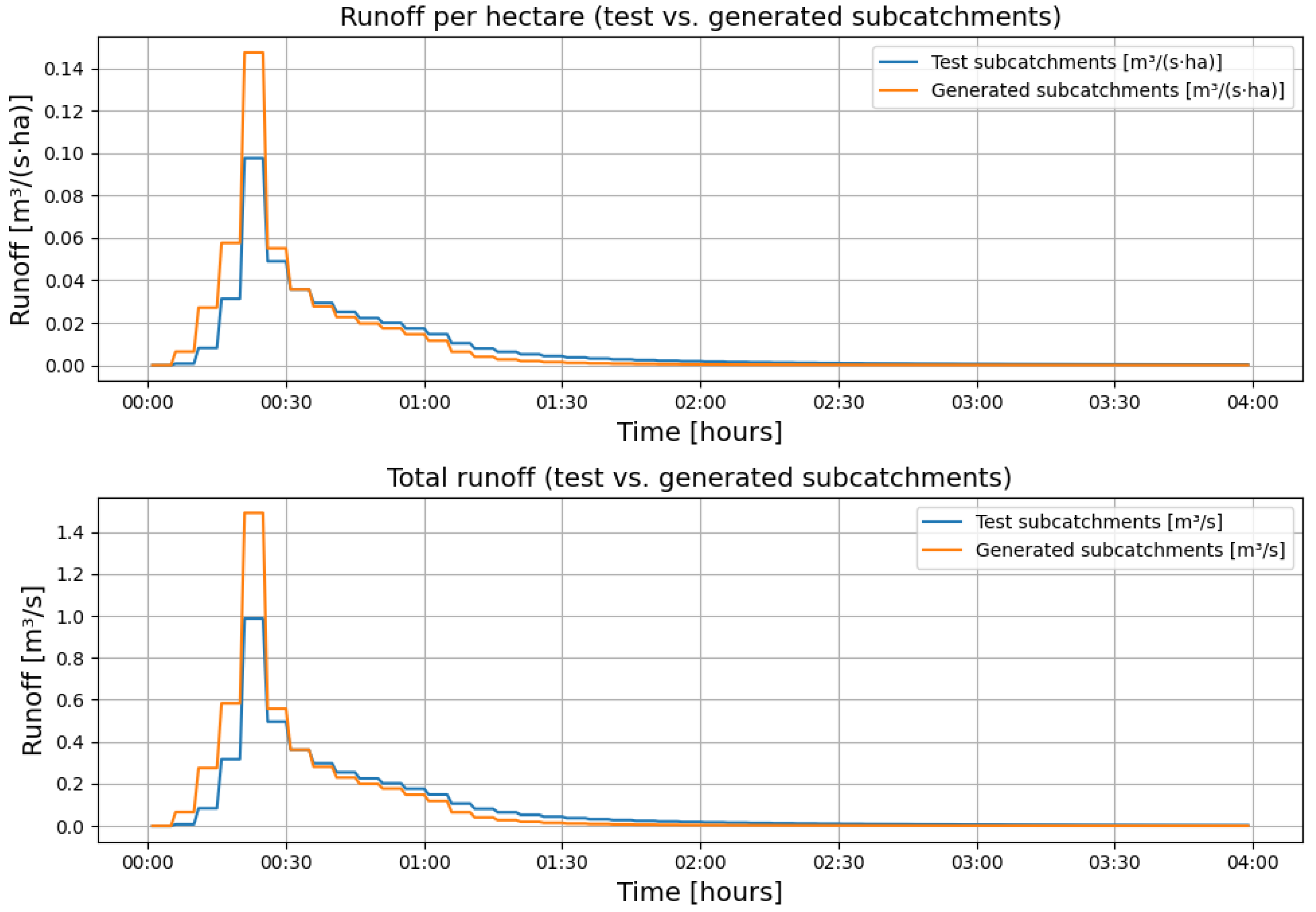
During the 60-min design storm, the test basin generated 126 m³/ha of runoff, 92.4 m³/ha of infiltration, and a peak discharge of 0.10 m³/s/ha. The generated basin yielded 140.1 m³ ha⁻¹, 88.8 m³ ha⁻¹, and 0.147 m³ s⁻¹ ha⁻¹, respectively. This corresponds to Mean Absolute Percentage Errors (MAPEs) of 15.9% for runoff, 19.2% for infiltration, and 37.7% for peak flow. A similar pattern was observed in the 120-min storm (runoff MAPE 15.7%, infiltration MAPE 19.2%, peak flow MAPE 29.4%).

3.1. Volume Validation

Agreement between test and generated time series was quantified with Nash–Sutcliffe efficiency (NSE), coefficient of determination (R²), percent bias (PBIAS), root mean square error (RMSE), and the above MAPE values (

Table 8. Statistical comparison of calibrated (P) and generated (G) total-runoff series.

Design Storm	Design Storm	NSE	R2	PBIAS (%)	RMSE (m3 ha−1)	MAPE (%)
Runoff	60 min	0.91	0.99	11.4	14.5	15.9
Runoff	120 min	0.92	0.99	10.9	16.5	15.7
Infiltration	60 min	0.91	0.94	−3.9	10.3	19.4
Infiltration	120 min	0.91	0.94	−3.9	11.9	19.2

).

Runoff metrics indicate excellent skill: NSE ≈ 0.92, R² = 0.99, and volume MAPE ≈ 16%. A positive PBIAS of about +11% confirms the conservative overprediction already noted. Infiltration shows similarly strong performance (NSE = 0.91, R² = 0.94) with a small negative PBIAS (~−4%). All statistics fall within the “very good” range recommended for preliminary urban-drainage analyses [62].

3.2. Peak-Flow Bias

Figure 11 and Figure 12 show that generated hydrographs peak earlier and higher than test hydrographs. This bias originates from the square-footprint assumption, which yields greater hydraulic width than is typical for elongated urban catchments. Reducing width in a sensitivity test lowered peak-flow MAPE below 15% while leaving volume metrics in Table 8 virtually unchanged, confirming that width had a decisive impact.

Figure 11. Runoff hydrographs for the 60-min Euler Type II rainfall event, comparing the test catchments (P1–P37) and the generated catchments (G1–G37). The generated catchments show a higher and earlier peak runoff due to a larger Width parameter, which accelerates the concentration of runoff. The similarity in overall hydrograph shapes indicates effective replication of hydrological responses by the generated catchments under shorter-duration, high-intensity rainfall.

Figure 11. Runoff hydrographs for the 60-min Euler Type II rainfall event, comparing the test catchments (P1–P37) and the generated catchments (G1–G37). The generated catchments show a higher and earlier peak runoff due to a larger Width parameter, which accelerates the concentration of runoff. The similarity in overall hydrograph shapes indicates effective replication of hydrological responses by the generated catchments under shorter-duration, high-intensity rainfall.

4. Conclusions

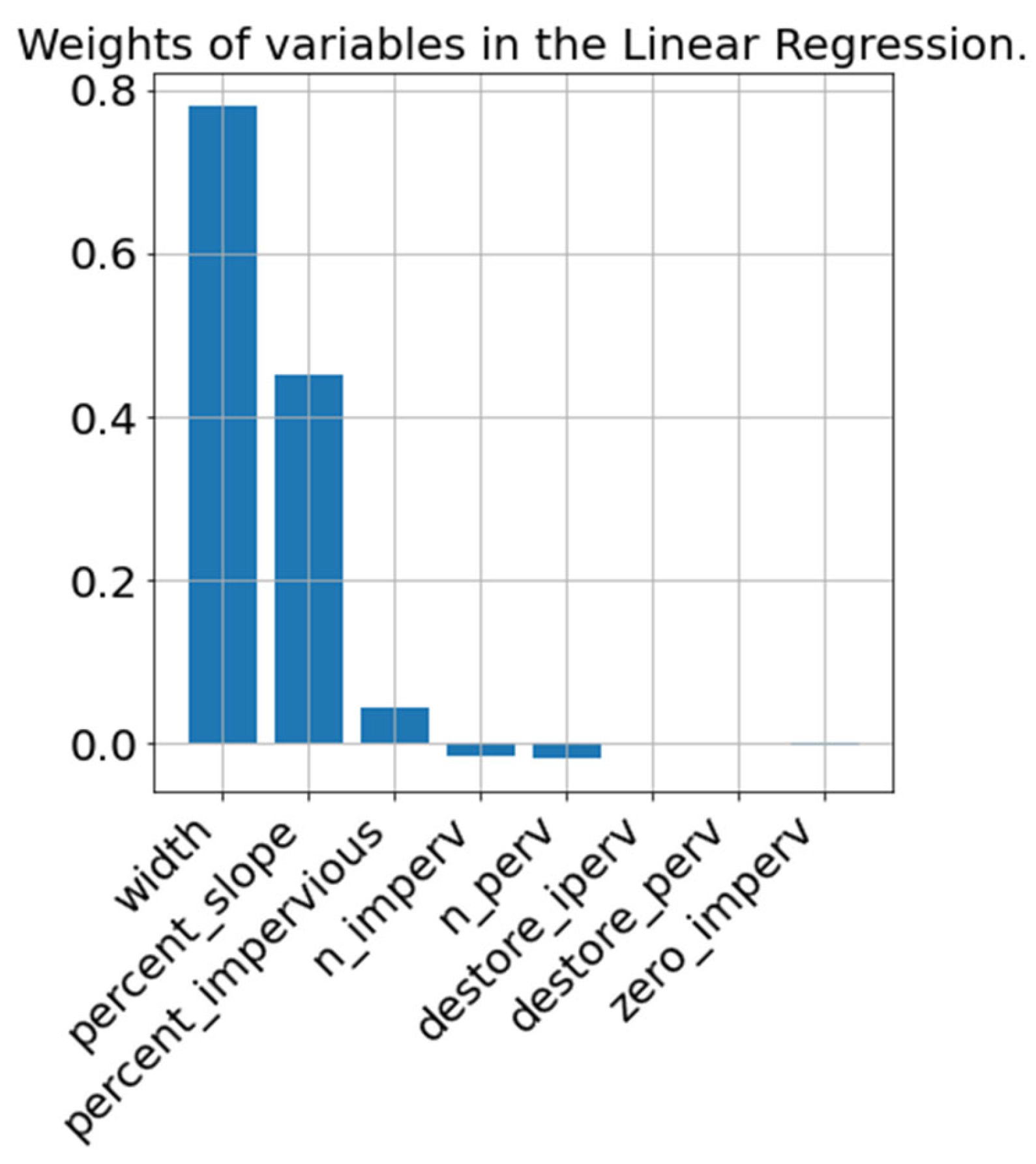
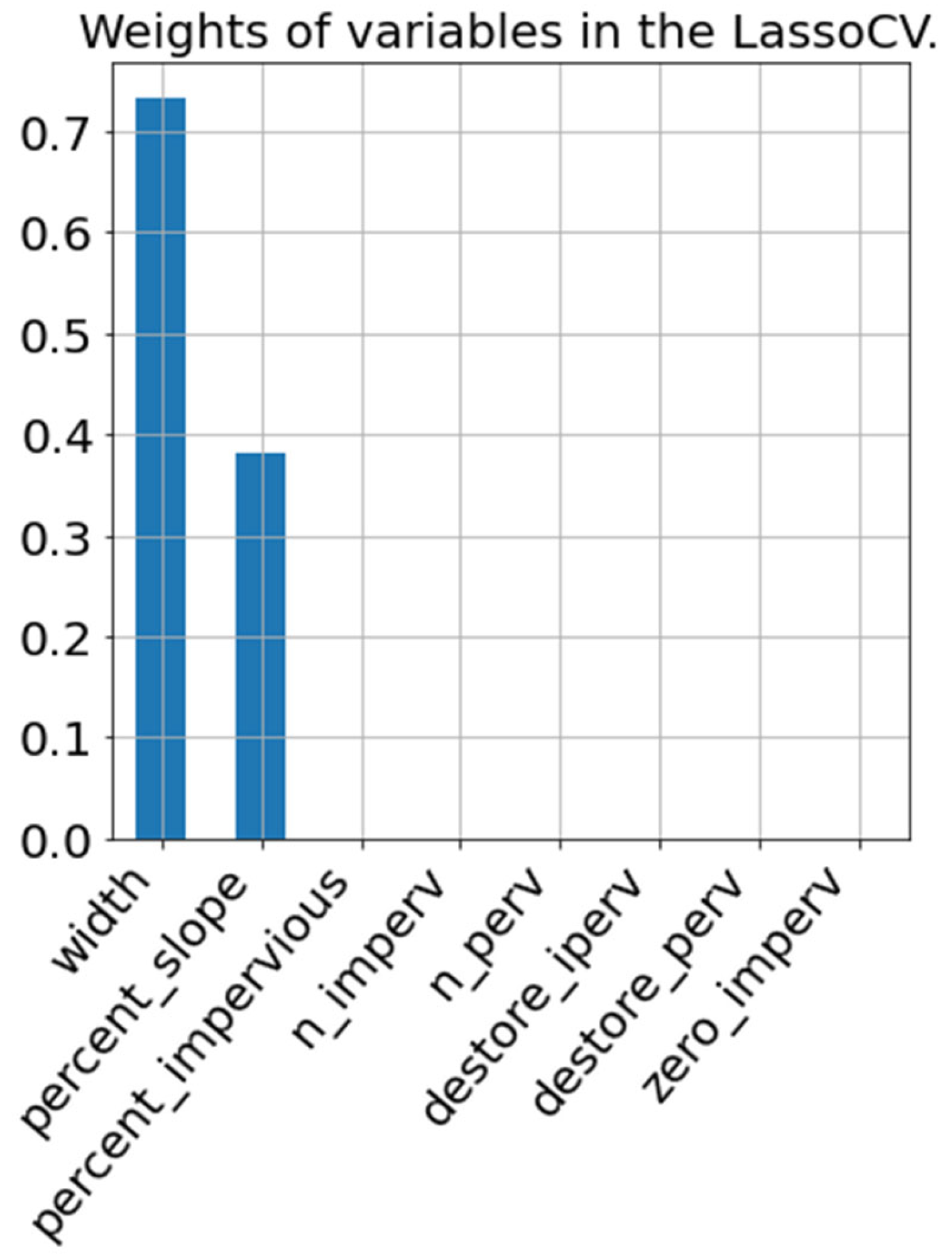
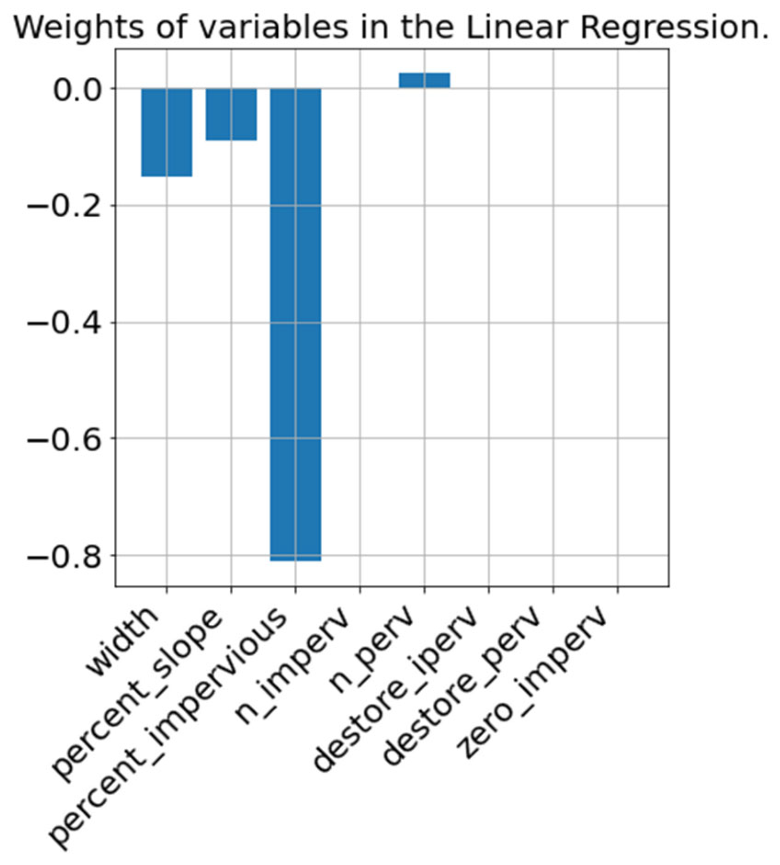
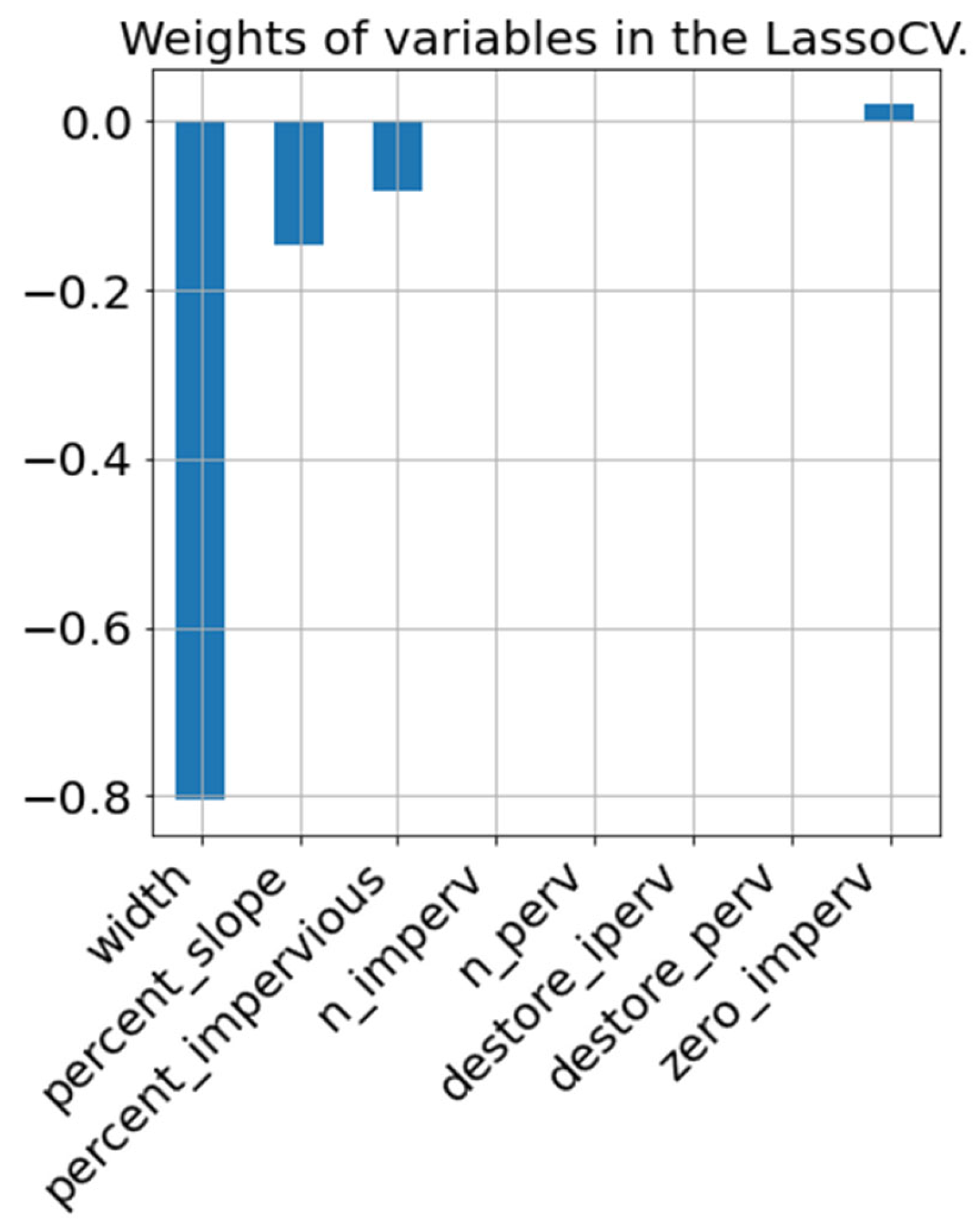
The SWMM tool offers an accurate approach to modeling rainfall events within catchment areas by considering parameters that realistically represent real-world conditions. The analysis of catchment features reveals that the width of the flow path, slope, and imperviousness are the most significant factors affecting runoff from the catchment.

The catchment generator was built based on the feature analysis conducted and surface runoff studies available in the literature. Parameterized categories of land cover and landforms were used as a basis for preparing fuzzy logic controller rules. Mapping typical storage and Manning’s coefficients simplified the catchment configuration process. The use of fuzzy logic rules allows modification of the system to adapt the categories to specific conditions. The construction of membership functions makes it possible to improve the accuracy of calculations and adapt the tool for different uses. Accurate representation of the actual condition of the catchment is possible through subsequent editing of the catchment in the SWMM GUI; no difficulties were observed with editing the *.inp file.

Performance analysis demonstrates that fuzzy logic effectively models and represents expert knowledge in hydrological systems. However, the results also reveal a consistent overestimation pattern in the generated catchments’ runoff values compared to the test catchment. With Mean Absolute Percentage Error (MAPE) values of 15–16% for runoff and approximately 19% for infiltration, the generated catchments closely approximate the hydrological behavior of the test catchment. Nevertheless, the higher MAPE values for peak runoff—37.7% for the 60-min event and 29.4% for the 120-min event—indicate a significant discrepancy in peak flow rates. At the concept stage, this conservative overprediction is acceptable, even desirable, because oversizing conduits is safer than undersizing them; however, peak-flow bias should be removed before detailed design.

The differences in peak runoff values are primarily attributed to the larger Width parameter calculated for the generated catchments. RCG assumes square-shaped catchments (as detailed in Table 5), resulting in a calculated width that does not accurately represent urban catchments with numerous paved streets and walkways. In urban environments, these impervious surfaces channelize runoff, leading to faster flow paths and higher peak runoff rates. The simplified assumption of square catchments in the RCG may not capture this complex drainage effectively, leading to the observed overestimation of peak runoff in the generated catchments.

Additionally, these discrepancies can be attributed to certain limitations of the RCG. One such limitation is the maximum imperviousness value that the RCG can assign. For example, the test catchment P17 has 100% impervious surfaces, whereas the generated catchment G17 has a maximum imperviousness of 86.7%, which is the highest value the RCG can generate based on its internal settings (as outlined in Figure 3). This limitation prevents the RCG from fully replicating catchments that are entirely urbanized or have fully paved surfaces. Consequently, this leads to underestimations in runoff volumes in highly impervious areas, as the model cannot assign values above the predefined maximum. Another limitation is related to the slope values. The test catchments have slope values ranging from 0.1% to 0.5%, while the RCG’s minimum slope value is 0.33%, as per the defined categories (see Figure 2). This means that the RCG is unable to generate catchments with the lowest slope values observed in the test catchments, potentially affecting the accuracy of runoff predictions in areas where gentle slopes dominate. Consequently, this limitation might lead to slight overestimations of flow velocity and runoff in flatter catchments, where lower slopes should slow down overland flow and allow for more infiltration.

Despite these limitations, the RCG fulfills its primary function as a tool for rapid prototyping of catchments. It provides a quick and efficient means to generate catchment models based on general land use and landform categories. However, the generated catchments require calibration and careful consideration of specific hydrological parameters, such as surface imperviousness, slope, and flow path geometry. These adjustments are necessary to enhance the accuracy of the models, particularly in urban environments where complex flow patterns and highly impervious surfaces are common. Therefore, while RCG serves as a valuable starting point for hydrological analysis, it should be viewed as a precursor to more detailed modeling efforts that incorporate site-specific data and refinements.

The proposed catchment generator has proven to be an effective tool for rapid SWMM prototyping, cutting model setup time from hours to seconds. Written in Python and relying only on open-source libraries such as SWMMIO and Scikit–Fuzzy, it remains accessible to a broad range of users. Future work will extend the fuzzy-logic rule base with an optional low-impact development (LID) layer, allowing users to prototype source control scenarios without any manual edits to the model file. Planned tests will also vary precipitation intensity and duration and incorporate additional land use types.

While this study focused on the “flats and plateaus” landform type, the fuzzy logic controller can accommodate nine different landform categories. Exploring other categories, such as “lowlands” or “mountains”, could reveal different runoff characteristics and calibration needs. For instance, using steeper terrain may introduce slope-related challenges that were not addressed in this study. As such, additional calibration steps may be necessary to evaluate the model’s performance across different landforms. These terrains, often with more complex hydrological behaviors, could present new challenges in mapping watershed characteristics. While the model has performed well for “flats and plateaus”, further exploration across other categories would provide a more comprehensive understanding of its strengths and limitations. Expanding to other landform types would also offer opportunities to optimize the model’s ability to map linguistic variables to numerical values.

References

1. Zeng, Z.; Yuan, X.; Liang, J.; Li, Y. Designing and implementing an SWMM-based web service framework to provide decision support for real-time urban stormwater management. Environ. Model. Softw. 2021, 135, 104887. [Google Scholar] [CrossRef]
2. Calvin, K.; Dasgupta, D.; Krinner, G.; Mukherji, A.; Thorne, P.W.; Trisos, C.; Adedoyin, J.A.; Al Busaidi, H.; Bustamante, M.; Cavicchioli, R.; et al. Climate Change 2023: Synthesis Report, Summary for Policymakers; Lee, H., Romero, J., Eds.; Contribution of Working Groups I, II and III to the Sixth Assessment Report of the Intergovernmental Panel on Climate Change; IPCC: Geneva, Switzerland, 2023; pp. 1–34. [Google Scholar]
3. Szeląg, B.; Suligowski, R.; De Paola, F.; Siwicki, P.; Majerek, D.; Łagód, G. Influence of urban catchment characteristics and rainfall origins on the phenomenon of stormwater flooding: Case study. Environ. Model. Softw. 2022, 150, 105335. [Google Scholar] [CrossRef]
4. Fletcher, T.; Coleman, R.; Bos, D.; Lavau, S.; Russell, K.; Burns, M.J.; Costello, R.; Bergmann, D.; Wallis, E. Combining community and technology to turn stormwater into water supply, flood mitigation and provision of environmental flow. In Proceedings of the Novatech 2023: 11e Conférence Internationale sur l’eau Dans la Ville, Lyon, France, 3–7 July 2023. [Google Scholar]
5. Li, F.; Yan, X.F.; Duan, H.F. Sustainable design of urban stormwater drainage systems by implementing detention tank and LID measures for flooding risk control and water quality management. Water Resour. Manag. 2019, 33, 3271–3288. [Google Scholar] [CrossRef]
6. Wong, T.H.; Brown, R.R. The water sensitive city: Principles for practice. Water Sci. Technol. 2009, 60, 673–682. [Google Scholar] [CrossRef]
7. Liu, Q.; Cui, W.; Tian, Z.; Tang, Y.; Tillotson, M.; Liu, J. Stormwater management modeling in “Sponge City” construction: Current state and future directions. Front. Environ. Sci. 2022, 9, 816093. [Google Scholar] [CrossRef]
8. Zhang, F. Evaluating public organization performance under extreme weather events: Does organizational adaptive capacity matter? J. Environ. Manag. 2021, 296, 113388. [Google Scholar] [CrossRef]
9. Rossman, L.A. Storm Water Management Model User’s Manual, Version 5.0; Cincinnati: National Risk Management Research Laboratory, Office of Research and Development, US Environmental Protection Agency: Washington, DC, USA, 2010; p. 276.
10. Niazi, M.; Nietch, C.; Maghrebi, M.; Jackson, N.; Bennett, B.R.; Tryby, M.; Massoudieh, A. Storm water management model: Performance review and gap analysis. J. Sustain. Water Built Environ. 2017, 3, 04017002. [Google Scholar] [CrossRef]
11. Chow, V.T.; Maidment, D.R.; Mays, L.W. Applied Hydrology; McGraw-Hill: New York, NY, USA, 1988; pp. 530–537. [Google Scholar]
12. Beven, K.J.; Kirkby, M.J. A physically based, variable contributing area model of basin hydrology/Un modèle à base physique de zone d’appel variable de l’hydrologie du bassin versant. Hydrol. Sci. J. 1979, 24, 43–69. [Google Scholar] [CrossRef]
13. Singh, V.P.; Woolhiser, D.A. Mathematical modeling of watershed hydrology. J. Hydrol. Eng. 2002, 7, 270–292. [Google Scholar] [CrossRef]
14. Maidment, D.R. Arc Hydro: GIS for Water Resources; ESRI: Redlands, CA, USA, 2002. [Google Scholar]
15. Farhan, I.A.; Al-Bakri, F.T. Use of GIS and Remote Sensing to Assess Soil Erosion in an Arid to Semiarid Basin in Jordan. In Proceedings of the International Conference on Sediment Transport: Modeling in Hydrological Watersheds and Rivers, Istanbul, Turkey, 26–28 June 2012; Volume 5, pp. 145–152. [Google Scholar]
16. Karimi, P.; Bastiaanssen, W.G. Spatial evapotranspiration, rainfall and land use data in water accounting–Part 1: Review of the accuracy of the remote sensing data. Hydrol. Earth Syst. Sci. 2015, 19, 507–532. [Google Scholar] [CrossRef]
17. McDonnell, B.E.; Ratliff, K.; Tryby, M.E.; Wu, J.J.X.; Mullapudi, A. PySWMM: The Python Interface to Stormwater Management Model (SWMM). J. Open Source Softw. 2020, 5, 2292. [Google Scholar] [CrossRef] [PubMed]
18. Warsta, L.; Niemi, T.J.; Taka, M.; Krebs, G.; Haahti, K.; Koivusalo, H.; Kokkonen, T. Development and application of an automated subcatchment generator for SWMM using open data. Urban Water J. 2017, 14, 954–963. [Google Scholar] [CrossRef]
19. Niemi, T.J.; Kokkonen, T.; Sillanpää, N.; Setälä, H.; Koivusalo, H. Automated urban rainfall-runoff model generation with detailed land cover and flow routing. J. Hydrol. Eng. 2019, 24, 04019011. [Google Scholar] [CrossRef]
20. Thayer, D.J. The Ideal Stormwater Runoff Calculator and How to Apply It to Site Scale Planning of Federal Facilities. Ph.D. Thesis, University of Illinois at Urbana-Champaign, Champaign, IL, USA, 2016. [Google Scholar]
21. CNT. Green Values. Stormwater Management Calculator; Center for Neighborhood Technology: Chicago, IL, USA, 2009; Available online: https://greenvalues.cnt.org (accessed on 1 May 2025).
22. Yu, Z.; Aguayo, M.; Montalto, F.; Piasecki, M.; Behr, C. Developments in LIDRA 2.0: A planning level assessment of the cost-effectiveness of low impact development. In Proceedings of the World Environmental and Water Resources Congress 2010: Challenges of Change, Providence, RI, USA, 16–20 May 2010; pp. 3261–3270. [Google Scholar]
23. Mason, B.E.; Mullapudi, A.; Kerkez, B. StormReactor: An open-source Python package for the integrated modeling of urban water quality and water balance. Environ. Model. Softw. 2021, 145, 105175. [Google Scholar] [CrossRef]
24. Riaño-Briceño, G.; Barreiro-Gomez, J.; Ramirez-Jaime, A.; Quijano, N.; Ocampo-Martínez, C. MatSWMM–an open-source toolbox for designing real-time control of urban drainage systems. Environ. Model. Softw. 2016, 83, 143–154. [Google Scholar] [CrossRef]
25. Yang, Y.; Li, Y.; Huang, Q.; Xia, J.; Li, J. Surrogate-based multiobjective optimization to rapidly size low impact development practices for outflow capture. J. Hydrol. 2023, 616, 128848. [Google Scholar] [CrossRef]
26. Liu, C.; Li, W.; Zhao, C.; Xie, T.; Jian, S.; Wu, Q.; Xu, Y.; Hu, C. BK-SWMM flood simulation framework is being proposed for urban storm flood modeling based on uncertainty parameter crowdsourcing data from a single functional region. J. Environ. Manag. 2023, 344, 118482. [Google Scholar] [CrossRef]
27. Barreto-Neto, A.A.; de Souza Filho, C.R. Application of fuzzy logic to the evaluation of runoff in a tropical watershed. Environ. Model. Softw. 2008, 23, 244–253. [Google Scholar] [CrossRef]
28. Kazmierczak, B.; Kotowski, A.; Dancewicz, A. Verification of Storm Sewerage Sizing Methods with the Hydrodynamic Model SWMM 5.0 for the Municipality of Wroclaw. Ochr. Srodowiska 2012, 34, 25–31. (In Polish) [Google Scholar]
29. Vaze, J.; Jordan, P.; Beecham, R.; Frost, A.; Summerell, G. Guidelines for Rainfall-Runoff Modelling: Towards Best Practice Model Application; eWater Cooprative Research Centre: Melbourne, Australia, 2011. [Google Scholar]
30. Xu, C.Y. Hydrologic models. In Textbooks of Uppsala University; Department of Earth Sciences Hydrology: Uppsala, Sweden, 2002. [Google Scholar]
31. Nowakowska, M.; Kazmierczak, B.; Kotowski, A.; Wartalska, K. Identification, Calibration and Validation of Hydrodynamic Model of Urban Drainage System in the example of the City of Wroclaw. Ochr. Srodowiska 2017, 39, 51–60. (In Polish) [Google Scholar]
32. Huber, W.C.; Rossman, L.A.; Dickinson, R.E. EPA storm water management model, SWMM5. Watershed Models 2005, 338, 339–359. [Google Scholar]
33. Jehanzaib, M.; Ajmal, M.; Achite, M.; Kim, T.-W. Comprehensive review: Advancements in rainfall-runoff modelling for flood mitigation. Climate 2022, 10, 147. [Google Scholar] [CrossRef]
34. Shubinski, R.P.; Roesner, L.A. Linked Process Routing Models; Hydrologic Engineering Center: Davis, CA, USA, 1973. [Google Scholar]
35. Akan, A.O.; Houghtalen, R.J. Urban Hydrology, Hydraulics, and Stormwater Quality: Engineering Applications and Computer Modeling; John Wiley Sons: Hoboken, NJ, USA, 2003. [Google Scholar]
36. Cronshey, R. Urban Hydrology for Small Watersheds; U.S. Department of Agriculture, Soil Conservation Service, Engineering Division: Washington, DC, USA, 1986.
37. Rotshtein, A.P.; Rakytyanska, H.B. Applied Fuzzy Systems. In Fuzzy Evidence in Identification, Forecasting and Diagnosis; Springer: Berlin/Heidelberg, Germany, 2012; Volume 275, pp. 259–313. [Google Scholar]
38. Papas, P.J.; Ramsey, D.S.L.; Holmes, J.; Frood, D.; Lyon, S. Integrating data, expert opinion and fuzzy logic in the development of an index of wetland condition. Mar. Freshw. Res. 2022, 73, 1184–1195. [Google Scholar] [CrossRef]
39. Himanshu, P.; Chandra, L.; Ashutosh, B.; Janmejay, P.; Manoj, S. Rule Descriptions for Soil Quality and Soil Fertility Assessment using Fuzzy Control System. Int. J. Recent Technol. Eng. 2020, 8, 2277–3878. [Google Scholar] [CrossRef]
40. Gessler, P.E.; Moore, I.D.; McKenzie, N.J.; Ryan, P.J. Soil-landscape modelling and spatial prediction of soil attributes. Int. J. Geogr. Inf. Syst. 1995, 9, 421–432. [Google Scholar] [CrossRef]
41. Grosan, C.; Abraham, A. Fuzzy Expert Systems. Intell. Syst. A Mod. Approach 2011, 17, 219–260. [Google Scholar]
42. Mamdani, E.; Assilian, S. An experiment in linguistic synthesis with a fuzzy logic controller. Int. J. Hum. Comput. Stud. 1999, 51, 135–147. [Google Scholar] [CrossRef]
43. Brazález, E.; Macià, H.; Díaz, G.; Baeza_Romero, M.T.; Valero, E.; Valero, V. FUME: An air quality decision support system for cities based on CEP technology and fuzzy logic. Appl. Soft Comput. 2022, 129, 109536. [Google Scholar] [CrossRef]
44. Kandel, A. Fuzzy Mathematical Techniques with Applications; Addison-Wesley Longman Publishing Co.: Boston, MA, USA, 1986. [Google Scholar]
45. Tibshirani, R. Regression shrinkage and selection via the lasso. J. R. Stat. Soc. Ser. B Stat. Methodol. 1996, 58, 267–288. [Google Scholar] [CrossRef]
46. Pedregosa, F.; Varoquaux, G.; Gramfort, A.; Michel, V.; Thirion, B.; Grisel, O.; Duchesnay, É. Scikit-learn: Machine learning in Python. J. Mach. Learn. Res. 2011, 12, 2825–2830. [Google Scholar]
47. Zou, H.; Hastie, T. Regularization and variable selection via the elastic net. J. R. Stat. Soc. Ser. B Stat. Methodol. 2005, 67, 301–320. [Google Scholar] [CrossRef]
48. Soil Survey Staff. Soil Survey Manual, 12th ed.; U.S. Department of Agriculture: Washington, DC, USA, 2017. Available online: https://www.nrcs.usda.gov (accessed on 1 May 2025).
49. Li, X.; Gao, J.; Guo, Z.; Yin, Y.; Zhang, X.; Sun, P.; Gao, Z. A study of rainfall-runoff movement process on high and steep slopes affected by double turbulence sources. Sci. Rep. 2020, 10, 9001. [Google Scholar] [CrossRef] [PubMed]
50. Kazemi, H. Evaluating the Effectiveness and Hydrological Performance of Green Infrastructure Stormwater Control Measures. Ph.D. Thesis, University of Louisville, Louisville, KY, USA, December 2014. Available online: https://ir.library.louisville.edu/etd/1744/ (accessed on 1 May 2025).
51. Yao, L.; Wei, W.; Chen, L. How does imperviousness impact the urban rainfall-runoff process under various storm cases? Ecol. Indic. 2016, 60, 893–905. [Google Scholar] [CrossRef]
52. U.S. Geological Survey. Slope Map of Part of West-Central King County, Washington. 1975. Available online: https://pubs.usgs.gov/imap/0852e/plate-1.pdf (accessed on 1 May 2025).
53. Meybeck, M.; Green, P.; Vörösmarty, C. A new typology for mountains and other relief classes. Mt. Res. Dev. 2001, 21, 34–45. [Google Scholar] [CrossRef]
54. Mandarino, A.; Faccini, F.; Terrone, M.; Paliaga, G. Anthropogenic landforms and geo-hydrological hazards of the Bisagno Stream catchment (Liguria, Italy). J. Maps 2021, 17, 122–135. [Google Scholar] [CrossRef]
55. Stępniewski, K.; Demczuk, P.; Rodzik, J.; Siwek, K. Związki między opadem deszczu a spływem powierzchniowym i spłukiwaniem gleby na poletkach doświadczalnych o różnym użytkowaniu (Guciów–Roztocze Środkowe). Pr. I Stud. Geogr. 2010, 45, 229–241. (In Polish) [Google Scholar]
56. U.S. Environmental Protection Agency. Report on the Environment (ROE): Land Cover. Available online: https://cfpub.epa.gov/roe/definitions.cfm?i=492023 (accessed on 25 March 2025).
57. Multi-Resolution Land Characteristics (MRLC) Consortium. In National Land Cover Database (NLCD) Class Legend and Description. U.S. Geological Survey. Available online: https://www.mrlc.gov/data/legends/national-land-cover-database-class-legend-and-description (accessed on 25 March 2025).
58. Łachowski, W. Analiza zmian powierzchni nieprzepuszczalnych w badaniu suburbanizacji na przykładzie Poznania. Urban Dev. Issues 2020, 66, 45–58. (In Polish) [Google Scholar] [CrossRef]
59. European Environment Agency. CORINE Land Cover Nomenclature—Illustrated Guide (CLC2018). Copernicus Land Monitoring Service. 2019. Available online: https://land.copernicus.eu/content/corine-land-cover-nomenclature-guidelines/docs/pdf/CLC2018_Nomenclature_illustrated_guide_20190510.pdf (accessed on 25 March 2025).
60. Tarka, R. 1995-Optymalizacja pomiarów hydrologicznych w wyznaczaniu odpływu podziemnego metodą źródeł reprezentatywnych. Gosp. Wodna 1995, 3, 6–13. (In Polish) [Google Scholar]
61. Guo, J.C.; Urbonas, B. Conversion of Natural Watershed to Kinematic Wave Cascading Plane. J. Hydrol. Eng. 2009, 14, 839–846. [Google Scholar] [CrossRef]
62. Moriasi, D.N.; Arnold, J.G.; Van Liew, M.W.; Bingner, R.L.; Harmel, R.D.; Veith, T.L. Model evaluation guidelines for systematic quantification of accuracy in watershed simulations. Trans. ASABE 2007, 50, 885–900. [Google Scholar] [CrossRef]
Figure 1. Weights of variables in linear regression with total runoff as the target.
Water 17 01820 g001
Figure 2. Feature importance for runoff using the LassoCV model.
Water 17 01820 g002
Figure 3. Weights of variables in linear regression with total infiltration as the target.
Water 17 01820 g003
Figure 4. Feature importance for infiltration using the LassoCV model.
Water 17 01820 g004
Figure 5. Workflow of the Rapid Catchment Generator (RCG). User inputs (left) are read by a runner script, passed to a fuzzy logic controller that classifies the catchment, evaluates membership functions and rules, and returns hydraulic width, slope, and imperviousness. The file manager module inserts these parameters into the appropriate sections of the SWMM .inp file (add catchment, sub-areas, coordinates, and infiltration) and saves the file, after which the loop is ready for the next catchment descriptor set. This automated loop enables rapid, code-free prototyping of multiple subcatchments.
Water 17 01820 g005
Figure 6. Fuzzy logic controller response surface for catchment slope, illustrating the impact of all possible combinations of land cover types (Table 4) and landform types (Table 3) on the calculated slope percentage.
Water 17 01820 g006
Figure 7. Fuzzy logic controller response surface for catchment imperviousness, illustrating the impact of all possible combinations of land cover types (Table 4) and landform types (Table 3) on the calculated impervious area percentage.
Water 17 01820 g007
Figure 8. Test catchment area in Wrocław, showing subcatchments (P1–P37), sewer collectors, and outflow to the Odra River; some elements adapted from Kazmierczak and Kotowski [28].
Water 17 01820 g008
Figure 9. Euler Type II design rainfall for Wroclaw with a return period of 3 years and a duration of 60 min.
Water 17 01820 g009
Figure 10. Euler Type II design rainfall for Wroclaw with a return period of 3 years and a duration of 120 min.
Water 17 01820 g010
Figure 12. Runoff hydrographs for the 120-min Euler Type II rainfall event, comparing the test and generated catchments. Similar to the 60-min event, the generated catchments exhibit higher peak runoff owing to the larger Width parameter. The extended duration results in a broader hydrograph peak, but the generated catchments continue to effectively replicate the hydrological behavior of the test catchments under longer-duration rainfall conditions.
Water 17 01820 g012