Ecological Assessment of Rivers Under Anthropogenic Pressure: Testing Biological Indices Across Abiotic Types of Rivers

Abstract

The ecological assessment of rivers under the Water Framework Directive (WFD) requires the use of biological quality elements (BQEs) across defined abiotic types of rivers. However, limited evidence exists on how well biological indices perform across multiple typological classes, particularly under the influence of complex, overlapping stressors. This study evaluated the diagnostic performance of four biological indices (IO—diatoms, MIR—macrophytes, MMI_PL—benthic macroinvertebrates, and EFI + PL—fish) in 16 river sites in southern Poland. These were classified into four abiotic types (5, 6, 12, and 17) and subjected to varying levels of human pressure. Biological, physical and chemical, and hydromorphological data were collected along environmental gradients including conductivity, nutrient enrichment, and habitat modification. Statistical analyses were used to evaluate patterns in community composition and index responsiveness. The IO and MMI_PL indices were the most consistent and sensitive in distinguishing between reference and degraded river conditions. MIR and EFI + PL were more variable, especially in lowland rivers, and showed stronger associations with habitat structure and oxygen levels. Conductivity emerged as a key driver of biological responses across all BQEs, with clear taxonomical shifts observed. The results support the need to consider both typological context and local environmental variation in ecological classification. The findings underscore the need for typology-aware, pressure-specific biomonitoring strategies that combine multiple organism groups and integrate continuous environmental variables. Such approaches can enhance the ecological realism and diagnostic accuracy of river assessment systems, supporting more effective water resource management across diverse hydroecological contexts.

1. Introduction

Rivers and streams are among the most threatened ecosystems worldwide, facing degradation from a variety of anthropogenic pressures, including nutrient enrichment, hydromorphological alteration, organic pollution, invasive species, and climate change [1,2,3]. These pressures, acting individually or in combination, cause decreases in biodiversity, the homogenisation of biotic communities, and the degradation of ecological functions [4,5,6,7]. Despite extensive research, the cumulative or interactive effects of multiple stressors remain poorly understood [8,9]. This is particularly true for rivers subjected to varying degrees of human impact, where disentangling the effects of local versus regional drivers is challenging [10,11].

To address the deteriorating condition of aquatic ecosystems, the European Union implemented the Water Framework Directive (WFD; [12]), which introduced a unified, ecology-based approach to flowing water assessment. The WFD requires the use of biological quality elements (BQEs), such as benthic diatoms (phytobentos), phytoplankton (only in large rivers), macrophytes, benthic macroinvertebrates, and fish, to determine ecological status. BQEs are core components of river monitoring and management [7,13,14]. Diatoms are valuable indicators due to their short life cycles, well-defined ecological tolerances (e.g., to pH, salinity, trophic status, and organic pollution), and sensitivity to short-term hydrochemical fluctuations [14,15,16,17]. Macrophytes are useful indicators of habitat structure, nutrient enrichment, and toxic pollution (e.g., herbicides and heavy metals), responding to both long-term and local changes in environmental conditions [14,18,19]. The use of benthic macroinvertebrates is highly recommended for water quality assessment due to their relatively low mobility, varied pollution tolerance, and year-round availability [14,20,21]. Fish, with long life spans and strong habitat dependence, are effective indicators of catchment-level impacts and hydromorphological integrity [14,22,23]. These elements are complemented by physical, chemical, and hydromorphological parameters. A central concept of the WFD is the comparison of observed biological conditions with reference conditions, thus separating anthropogenic change (synanthropisation) from natural succession [24,25].

The diagnostic strength of biological indices may vary depending on the abiotic typology of the water body. The type of river, defined by natural variation in hydromorphology, geology, and climate, modulates how aquatic communities respond to anthropogenic pressure. Existing studies have demonstrated that the same level of pollution may elicit different biological signals depending on whether a river is, for example, a sandy lowland stream or a high-gradient mountain watercourse [26,27,28,29]. However, despite the typology-based structure of the WFD, there remains limited empirical data to determine whether biological indices consistently reflect anthropogenic impacts across multiple types of rivers within the same biogeographic region.

Only a few studies have directly compared the relative sensitivity and robustness of BQEs across contrasting types of rivers under field conditions. Diatom, macrophyte, macroinvertebrate, and fish-based indices differ in their ecological focus and temporal integration, yet little is known about their comparative diagnostic value when applied simultaneously within rivers subjected to multiple interacting pressures. In particular, the question of whether index performance is typology-dependent and the extent to which certain indices may fail to detect stress in specific settings remain poorly addressed in Central European contexts. This constitutes a critical research gap, especially for systems affected by salinisation, organic pollution, and morphological alteration, which are common in post-industrial landscapes.

Our study explores the above issue by examining the performance of biological indices, applied in the rivers of southern Poland, representing distinct abiotic types, defined by WFD typology. Our specific objectives are to (1) quantify differences in the response of each BQE to environmental stress gradients across types of rivers; (2) compare the sensitivity and diagnostic consistency of the indices within and between abiotic types of rivers; and (3) evaluate the extent to which abiotic type of river mediates the detection of anthropogenic degradation. Achieving this will allow us to suggest typology-specific improvements in ecological assessment under the WFD framework.

2. Materials and Methods

2.1. Site Selection

In order to represent the gradient of anthropogenic pressure across different natural settings, this study was conducted in two major Central European ecoregions: the Central Highlands (Ecoregion 9) and the Carpathians (Ecoregion 10). Within these ecoregions, eight rivers located in Southern Poland were selected to represent four distinct abiotic types of rivers, as defined under the Water Framework Directive classification system [12,30].

According to relevant Regulations [31,32], the selected types of rivers included the following: type 5 (RW_krz)—mid-altitude siliceous streams or small rivers (Bolina and Centuria rivers); type 6 (RW_wap)—mid-altitude calcareous streams or small rivers (Mitręga and Mleczna rivers); type 12 (RWf_krz)—flysch streams with siliceous substrate (Dziechcinka and Vistula rivers); and type 17 (PNp)—lowland sandy streams (Korzenica and Wiercica rivers) (

Table 1. Characteristics of the study sites.

Characteristic	Type 5		Type 6		Type 12		Type 17
Selected rivers	Bolina	Centuria	Mitręga	Mleczna	Dziechcinka	Vistula	Korzenica	Wiercica
Geographical coordinates of the sampling sites	50°14.742 N, 19°06.078 E; 50°13.793 N, 19°05.142 E	50°21.920 N, 19°29.682 E; 50°24.879 N, 19°29.190 E	50°26.070 N, 19°17.956 E; 50°24.797 N, 19°22.779 E	50°07.018 N, 19°04.487 E; 52°09.754 N, 19°00.213 E	49°38.789 N, 18°52.025 E; 49°38.021 N, 18°50.828 E	49°38.728 N, 18°51.167 E; 49°37.190 N, 18°59.160 E	50°01.850 N, 19°05.839 E; 50°03.509 N, 18°56.804 E	50°52.471 N, 19°26.133 E; 50°41.117 N, 19°24.472 E
Main anthropogenic pressure in the upper course of the river	Salinisation from saline coal mine discharges, and river channel regulation	None	Dam reservoir, municipal sewage	Industrial and municipal sewage, and river regulation	None	None	Fish ponds and agricultural activity, municipal sewage	None
Main anthropogenic pressure in the lower course of the river	Salinisation from saline coal mine discharges, industrial and municipal wastewater, and river channel regulation	Organic pollution from agriculture and livestock grazing, as well as inputs from fish ponds	Dam reservoir, municipal sewage, river channel regulation	Salinisation from saline coal mine waters, industrial and municipal sewage, and river regulation	Riverbed regulation	Riverbed regulation, dam reservoir, municipal sewage	Fish ponds and agricultural activity	Agriculture, livestock grazing, and dam reservoirs

). To ensure clarity, the numbering of abiotic types of river (5, 6, 12, 17) is used consistently throughout the text, following the classification set out in Regulation [31]. Two sampling sites were designated for each river, resulting in a total of sixteen research sites. The sites were chosen to reflect a range of environmental degradation, from near-pristine to highly impacted conditions, particularly in relation to salinisation, organic pollution, and hydromorphological alterations. These pressures were previously documented and characterised in detail in our earlier studies [33,34,35,36,37].

2.2. Environmental Surveys

Comprehensive environmental characterisation was performed at each sampling site to capture local abiotic variation relevant to ecological status assessment. Field measurements included river width, depth, and flow velocity. The proportion of organic matter in the bottom sediments was determined using the standard loss-on-ignition method at 550 °C for 7 h [38]. Water samples were collected from the mid-channel point at each site immediately prior to biological sampling in 2018. Basic water parameters, including conductivity, total dissolved solids, pH, temperature, and dissolved oxygen, were measured in situ using handheld meters (HI-9811-5 Hanna Instruments, Woonsocket, RI, USA and CO-401 Elmetron, Zabrze, Poland). Laboratory analyses of chlorides, sulphates, iron, calcium, magnesium, total hardness, alkalinity total organic carbon (TOC), biological oxygen demand (BOD), and nutrients were performed using standard methods [39].

Hydromorphological assessment was conducted using the Hydromorphological Index for Rivers (HIR), in accordance with the national methodology [30,40]. This method integrates field data and GIS interpretation over 500-m river stretches and records both channel and valley characteristics. Two indices were derived from HIR metrics. The Hydromorphological Diversity Index (WRH) reflects the richness of natural features, while the Hydromorphological Transformation Index (WPH) quantifies anthropogenic modification. High WPH values indicate strong channel alteration, while high WRH values indicate morphological complexity and near-natural conditions. The grain size distribution of bottom sediments was analysed using a combination of sieve and hydrometer methods.

2.3. Biological Surveys

Biological surveys were conducted for all four BQEs in accordance with national monitoring protocols. Diatoms were sampled from at least 10 cm² of hard substrates (stones) or, where unavailable, from submerged macrophytes, following the procedure described by Zgrundo et al. [17]. The samples were cleaned using 10% hydrochloric acid to remove calcium carbonate and subsequently oxidised with 37% hydrogen peroxide to eliminate organic material. After multiple rinses in distilled water, cleaned suspensions were mounted on glass slides using the Naphrax^® mountant. Permanent slides were examined under light microscopes (Zeiss Axio Scope A1, Oberkochen, Germany and Nikon Eclipse E600, Melville, NY, USA). Identification and enumeration followed national standards, and the following indices were calculated: multimetric diatom index (IO), trophic index (TI), saprobic index (SI), and reference taxa abundance index (GR) [14,17,41,42].

Macrophyte surveys were carried out along 100 m river sections according to the Polish protocol based on the Macrophyte Index for Rivers (MIR) [19]. Only vascular plants and bryophytes growing in or rooted in the water were recorded. Taxa were identified at the species level where possible. Their relative abundance was estimated using a nine-point ordinal scale based on percentage cover. The MIR index was calculated from the field data to assess the ecological status of the rivers [14].

Benthic macroinvertebrates were sampled using the Multi-Habitat Sampling (MHS) method with a hydrobiological hand net (frame 25 cm × 25 cm, mesh size below 500 µm), as described by Bis and Mikulec [21]. Overall, 20 subsamples per site were collected proportionally from representative microhabitats, covering a total area of 1.25 m² [43]. Samples were preserved in 80% ethanol and identified at the family level in the laboratory. Based on the taxonomic data, the Polish multimetric index for macroinvertebrates (MMI_PL) was calculated [14]. This index integrates six metrics:

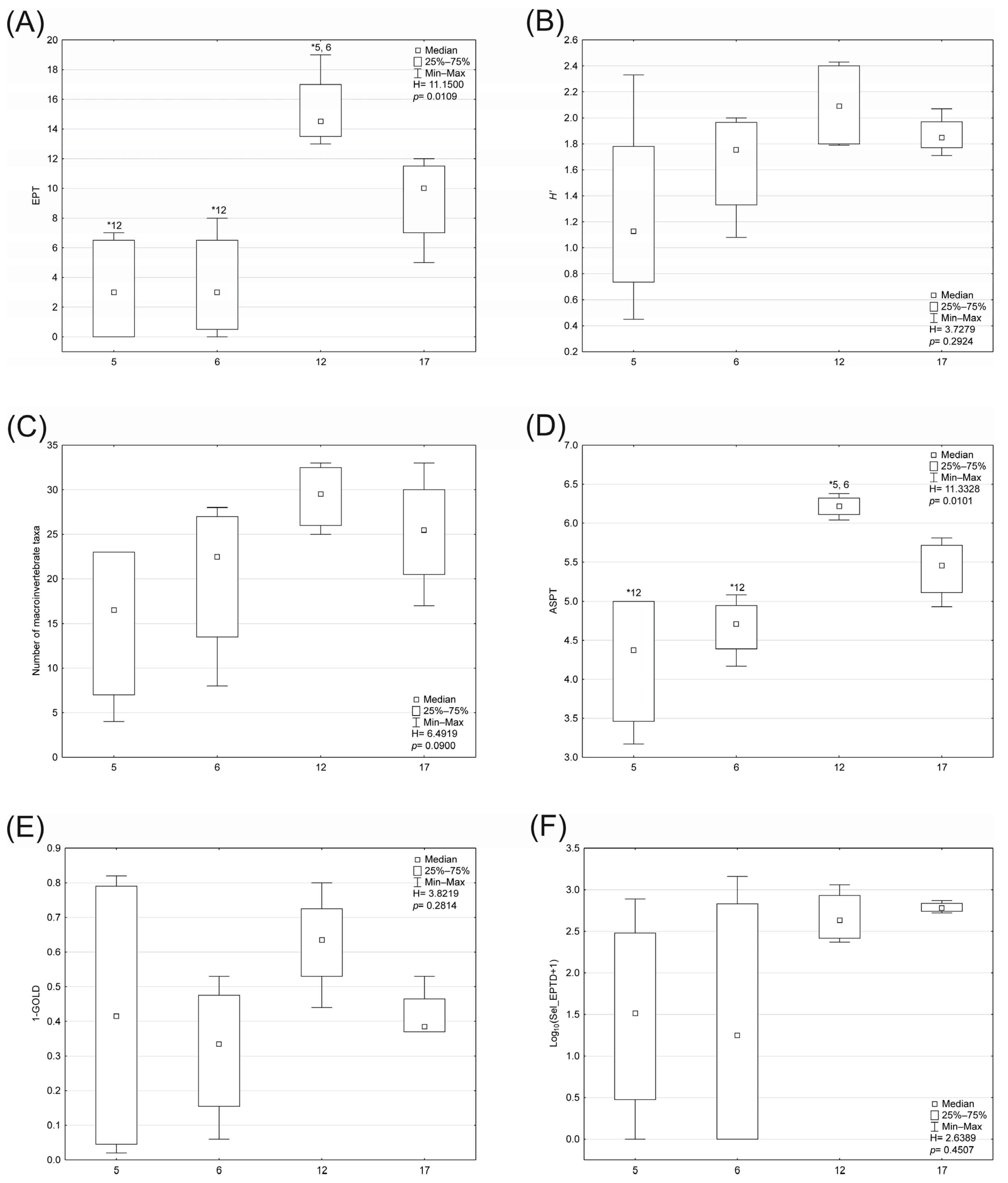
• EPT: the total number of families in the Ephemeroptera, Plecoptera and Trichoptera taxa.
• The Shannon–Wiener index (H′): H′ = −Σ(p_i) (ln p_i), where p_i = n_i/N, the proportion of individuals belonging to family is n_i, and N is the total number of macroinvertebrate individuals.
• The total number of macroinvertebrate families.
• ASPT (Average Score per Taxon): the value of the BMWP (Biological Monitoring Working Party) divided by the number of BMWP families present in the taxa list. All Oligochaeta were considered as one taxon.
• 1 − GOLD: 1 − (relative abundance of Gastropoda + Oligochaeta + Diptera).
• Log₁₀(Sel_EPTD + 1): log₁₀ (sum of individuals of the families Heptageniidae, Ephemeridae, Leptophlebiidae, Brachycentridae, Georidae, Polycentropodidae, Limnephilidae, Odontoceridae, Dolichopodidae, Stratiomyidae, Dixidae, Empididae, Athericidae, Nemouridae + 1).

Fish communities were sampled using backpack electrofishing equipment (IUP-12, 220–250 V, 7 A, Radet, Poznań, Poland) by wading upstream along the entire channel’s width. All collected fish were identified at the species level, measured for total length, and weighed. Native species were released after identification. Non-native species were removed from the ecosystem in accordance with ethical standards. The ecological status of each site was assessed using the Polish multimetric fish index (EFI + PL) [14,23].

2.4. Statistical Analyses

We tested the significance of differences in the median values of environmental variables, diversity metrics, and biological indices among the types of rivers using the Kruskal–Wallis one-way ANOVA and multiple comparison post hoc tests. The non-normal distribution of environmental variables was confirmed using the Lilliefors test, justifying the use of non-parametric procedures. All statistical analyses were conducted using Statistica software, version 13.1 (StatSoft Inc., Tulsa, OK, USA).

Canonical ordination techniques were used to explore relationships between environmental variables and the taxonomic composition of benthic macroinvertebrates, macrophytes, diatoms and fishes. Analyses were performed in CANOCO for Windows version 4.5 [44]. The choice of ordination method was based on gradient length, as determined by detrended correspondence analysis (DCA). Depending on the gradient length, either redundancy analysis (RDA) or canonical correspondence analysis (CCA) was applied to assess linear or unimodal relationships, respectively. Forward selection procedures were used to identify significant environmental predictors from a larger set of variables.

Taxa occurring at fewer than 10 percent of the sampling sites were excluded from the ordination analyses to minimise the influence of rare species [45]. Both biological and environmental datasets were log-transformed to improve linearity and reduce skewness. The statistical significance of biological and environmental relationships was evaluated using Monte Carlo permutation tests with 499 unrestricted permutations.

3. Results

3.1. Environmental Parameters Across Abiotic Types of Rivers

Environmental variables varied significantly among the four abiotic types of rivers. Differences in altitude, stream gradient, water temperature, conductivity, salinity, total dissolved solids, and nutrient-related ions, such as chlorides, sulphates, and nitrites, among types of rivers were statistically significant (p < 0.001,

Table 2. The physical and chemical parameters of the water, the morphology of the riverbed, and the results of the Kruskal–Wallis one-way ANOVA and multiple comparison post hoc tests (superscript ^a,b,c,d, denote significant differences among abiotic types of rivers: ^a type 5; ^b type 6; ^c type 12; ^d type 17).

Parameter	Type 5	Type 6	Type 12	Type 17	p-Value
Altitude [m a.s.l.]	257–343 c	236–317 c	415–748 a,b,d	215–309 c	0.0004
Stream gradient [‰]	3.00–10.89 d	2.83–3.98 c	45.59–177.50 b,d	2.00–3.92 a,c	0.0000
Width of the river bed [m]	3.600–7.480	2.636–8.100	3.247–12.450	1.190–13.100	0.1979
Depth of the river bed [m]	0.140–0.840 b	0.206–1.375 a	0.190–0.664	0.006–1.150	0.1116
Flow velocity [m s−1]	0.055–0.722	0.023–0.435 c	0.107–0.897 b	0.040–0.510	0.1979
Temperature [°C]	10.40–24.50 c	16.50–20.70 c	10.00–14.00 a,b	10.70–20.20	0.0000
pH	6.20–8.70	6.60–8.90	5.90–9.00	6.60–8.50	0.3884
Salinity [PSU]	0.17–25.70 c	0.25–10.58 c	0.02–0.08 a,b,d	0.17–0.29	0.0000
Conductivity [μS cm−1]	200–35,700 c	330–14,690 c	20–110 a,b,d	220–371 c	0.0000
Total dissolved solids [mg dm−3]	100–17,840 c	160–7350 c	10–50 a,b,d	100–187 c	0.0000
Chlorides [mg dm−3]	10–16,180 c	18–4060 c	4–10 a,b,d	10–23 c	0.0000
Dissolved oxygen [mg dm−3]	3.13–5.77	1.58–6.24 c	3.87–5.36 b	3.30–5.29	0.0054
Biochemical Oxygen Demand (BOD) [mg dm−3]	7–23	<3–4	<3–<3	<3–<3	0.2112
Sulfates [mg dm−3]	40–780 c,d	35–370 c,d	11–20 a,b	12–56 a,b	0.0000
Iron [mg dm−3]	0.01–0.91	0.14–1.97 c	0.00–0.60 b,d	0.01–2.17 c	0.0048
Ammonium [mg dm−3]	0.00–1.83	0.15–2.39 c	0.00–0.30 b	0.00–1.89	0.0089
Nitrites [mg dm−3]	0.000–2.687 c	0.012–2.702 c	0.000–0.020 a,b	0.000–0.250	0.0001
Nitrates [mg dm−3]	0.00–57.59	0.00–78.41	1.33–8.42	0.89–29.68	0.4459
Total nitrogen [mg dm−3]	1.9–4.1	1.5–5.9	0.81–1.10	1.2–4.1	0.1116
Phosphates [mg dm−3]	0.00–0.36 b	0.18–7.10 a,c	0.00–0.35 b	0.00–0.76	0.0040
Total phosphorus [mg dm−3]	0.100–0.240	0.065–0.460	0.064–0.190	0.140–0.180	0.5724
Total Organic Carbon (TOC) [mg dm−3]	2.5–3.5	7.8–11.0 c	<2.0–4.0 b	<2.0–8.1	0.1116
Total hardness [mg CaCO3 dm−3]	145–3700 c	155–1339 c	22–66 a,b,d	95–315 c	0.0005
Alkalinity [mg CaCO3 dm−3]	95–395 c	120–305 c	0.80–40 a,b,d	75–300 c	0.0001
Calcium [mg dm−3]	40–696 c	50–632 c	4–22 a,b,d	28–80 c	0.0004
Magnesium [mg dm−3]	0.12–476.64 c	0.73–157.63 c	0.12–8.25 a,b	0.61–76.26	0.0001
Organic matter [%]	0.55–20.51	0.83–30.46	1.75–3.93	0.64–1.43	0.1352
HIR	0.37–0.87	0.34–0.56	0.42–0.93	0.49–0.88	0.5724
WPH	1.0–52.5	51.5–56.5	5.5–79.5	13.5–47.0	0.0460
WRH	33.5–73.0	31.0–69.0	65.0–88.5	49.5–87.5	0.1116

). Flysch rivers (type 12) were located at the highest altitudes (415–748 m a.s.l.) and exhibited steep gradients (up to 177 ‰), low water temperature and low salinity (Table 2). In contrast, upland and anthropogenically altered rivers (especially the Bolina River, type 5) showed high conductivity and salinity values, with maximum conductivity reaching 35,700 μS cm⁻¹ and total dissolved solids exceeding 17,000 mg dm⁻³. These rivers were also distinguished by elevated concentrations of chlorides and sulphates. In terms of hydromorphological quality, rivers differed in the degree of physical transformation, as captured by the WPH index. Significantly elevated WPH values were observed in river types 5 and 6, indicating strong anthropogenic alteration, while flysch streams most often exhibited lower transformation levels and higher morphological diversity, reflected by higher WRH scores. Notably, some physical characteristics, such as river width, depth, flow velocity, and pH, did not differ significantly across types (p > 0.05), suggesting that pressure-related chemical and structural changes may exert stronger differentiation than basic morphometric features. The results of the composition of the grain size from bottom sediments are presented in Appendix A 

Table A1. Grain size compositions (fractions) of the bottom sediments from studied rivers.

Fraction mm (%)	Type 5		Type 6		Type 12		Type 17
Selected rivers	Bolina	Centuria	Mitręga	Mleczna	Dziechcinka	Vistula	Korzenica	Wiercica
<0.002	2.0–29.0	0.0–0.0	0.0–3.9	0.0–8.5	0.0–0.0	0.0–0.0	0.0–0.0	0.0–3.0
0.002–0.02	4.0–59.0	0.0–0.0	0.0–5.9	0.0–12.3	0.0–0.0	0.0–0.0	0.0–0.0	0.0–4.0
0.02–0.1	2.9–13.0	0.5–1.7	0.3–27.6	3.20–40.8	0.2–2.5	0.1–1.2	0.2–15.2	0.1–24.8
0.1–0.25	1.5–32.9	17.7–32.0	3.7–35.6	11.7–52.8	1.1–7.1	0.3–3.3	5.4–41.1	6.2–65.5
0.25–0.5	0.5–55.0	42.7–69.9	21.3–79.7	9.0–59.2	3.1–15.6	1.3–13.1	26.0–71.9	11.4–50.9
0.5–1	0.0–18.8	0.6–17.3	2.1–26.3	1.0–19.8	3.3–16.9	1.7–11.8	2.1–25.3	0.9–52.2
1–2	0.0–3.0	0.1–1.8	0.50–2.4	0.4–7.8	5.3–19.2	2.5–19.7	0.3–10.2	0.0–3.9
2–5	0.0–0.8	0.0–0.8	0.10–1.2	0.0–8.5	7.2–27.8	3.5–20.3	0.0–9.0	0.0–2.2
5–10	0.0–0.3	0.0–1.9	0.10–0.8	0.0–10.1	6.4–21.8	3.2–15.4	0.0–6.8	0.0–3.2
10–20	0.0–0.0	0.0–6.0	0.0–1.8	0.0–18.9	9.8–28.0	8.5–33.0	0.0–18.2	0.0–10.8
>20	0.0–0.0	0.0–20.4	0.0–28.7	0.0–6.1	1.1–38.0	7.9–72.9	0.0–40.3	0.0–20.8

.

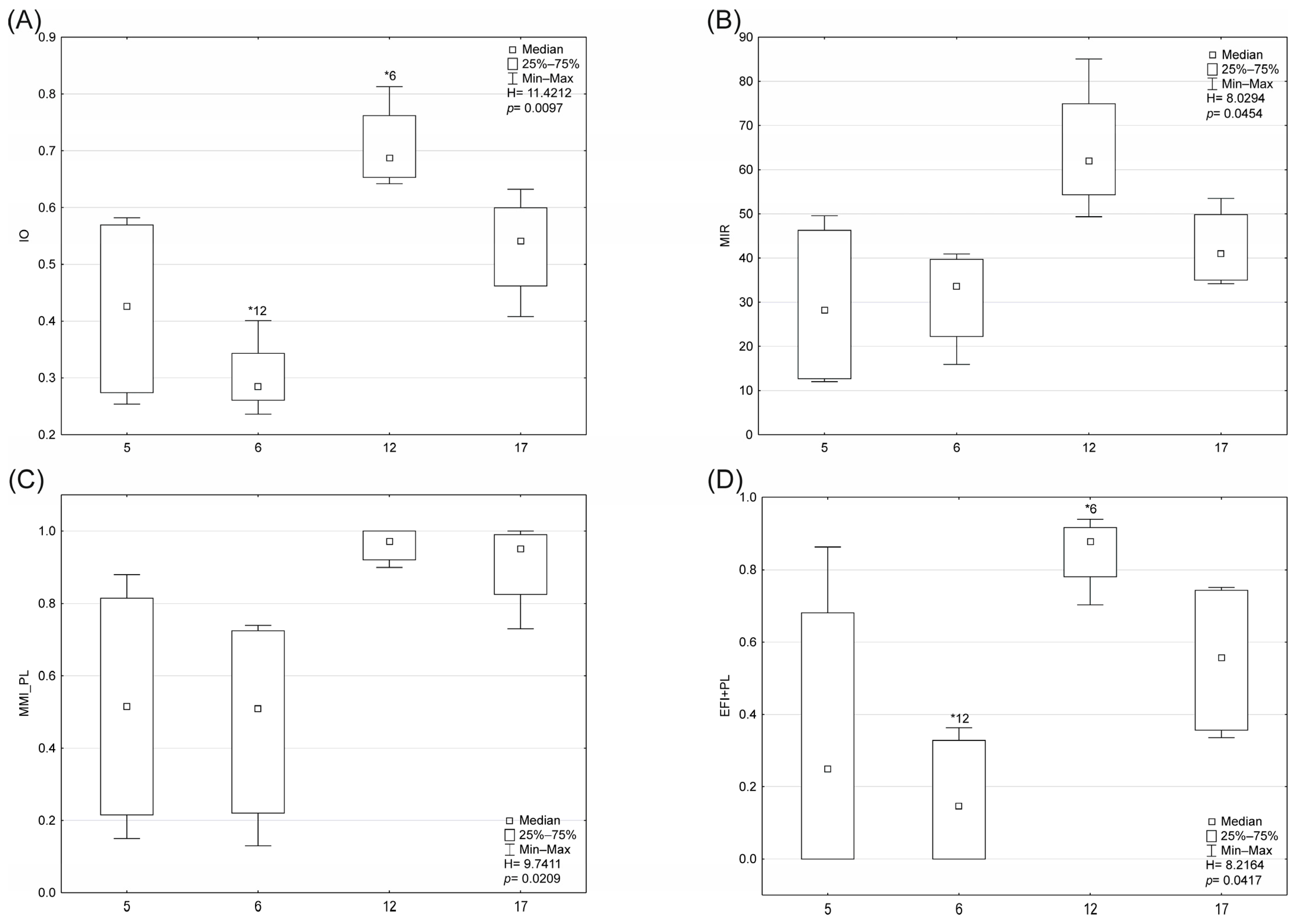
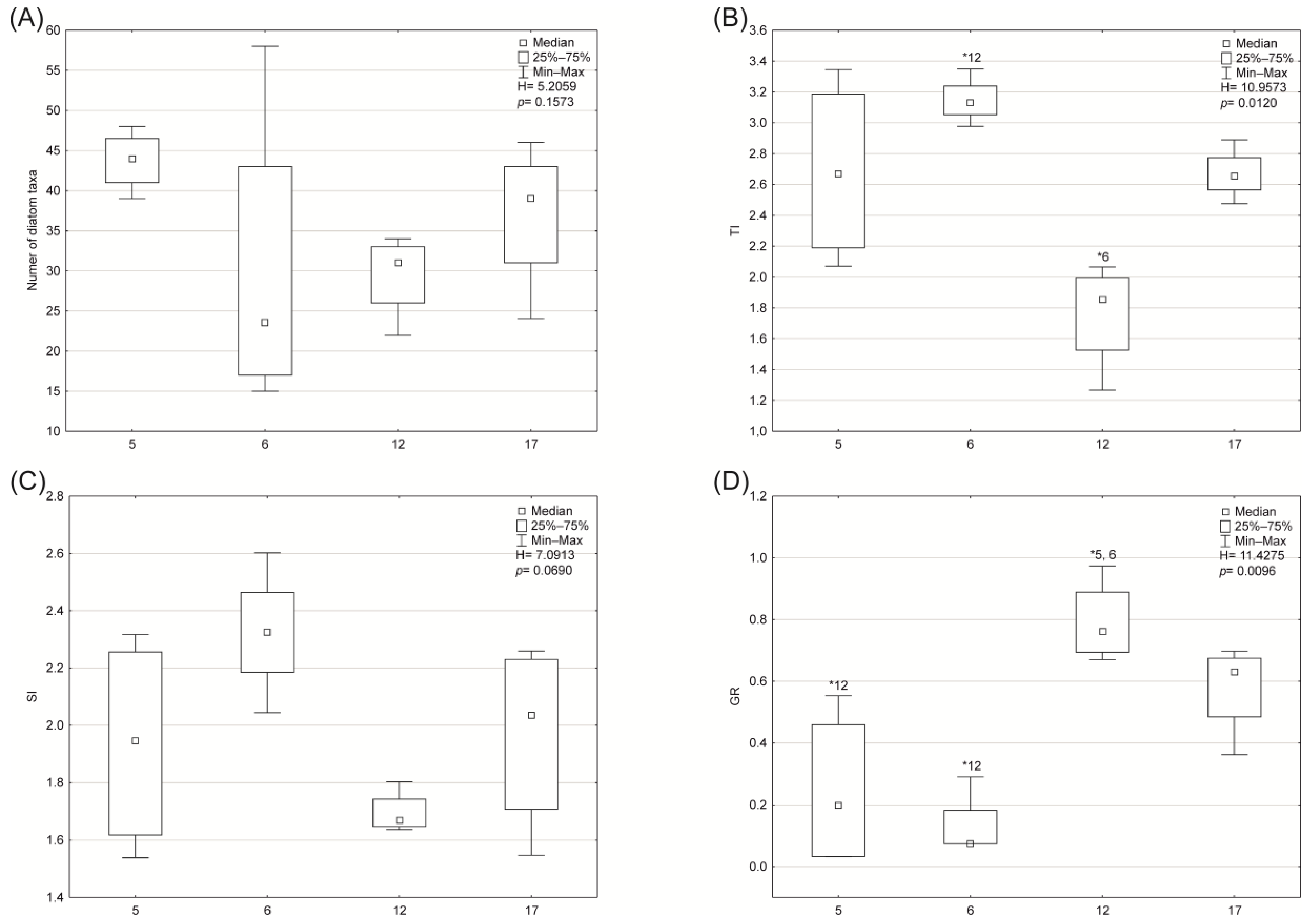
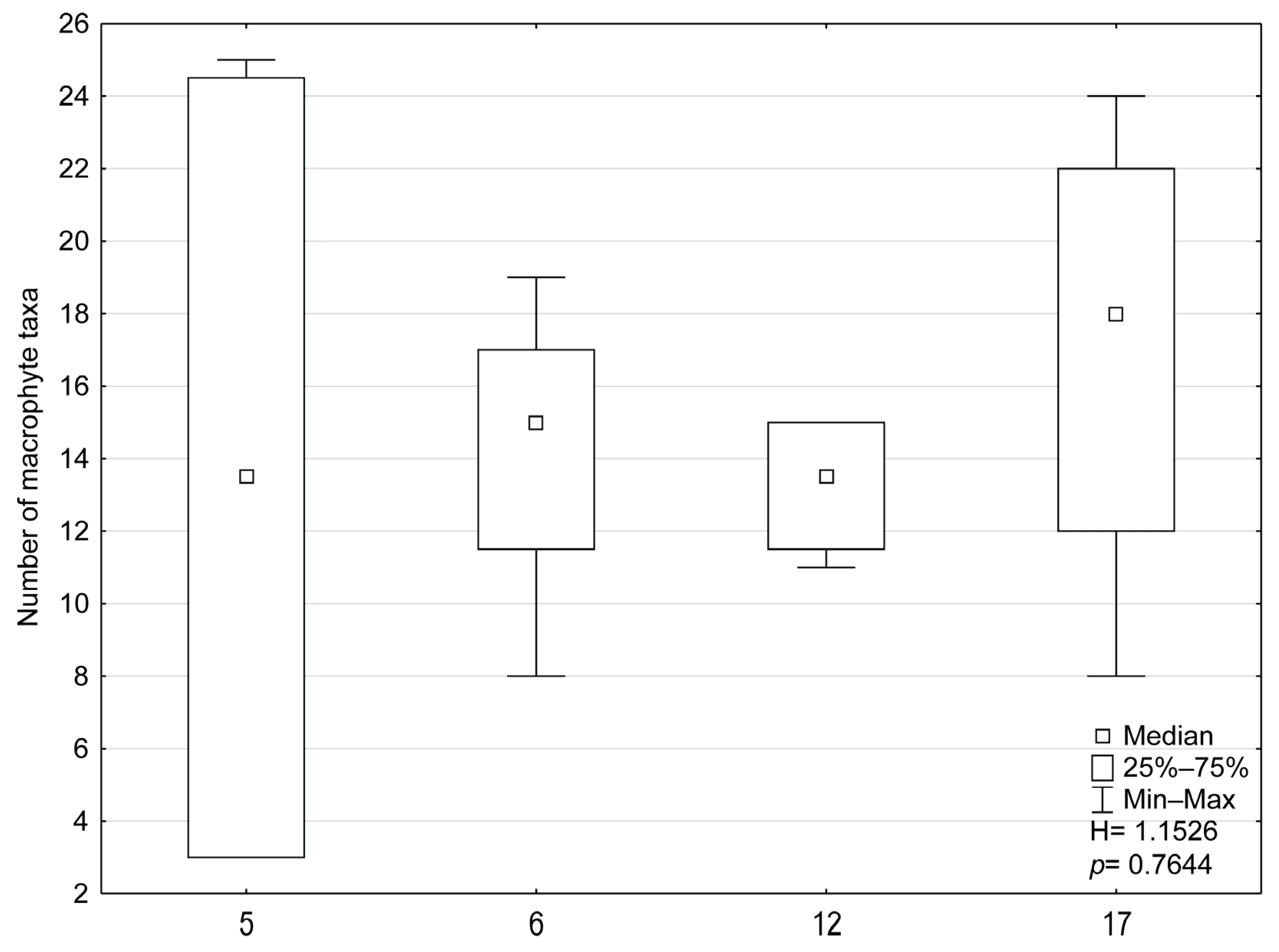
3.2. Biological Indices and Community Structure

The values of biological indices differed significantly among types of rivers, reflecting the variation in environmental conditions. According to Kruskal–Wallis tests, significant differences were found for the diatom IO index (p < 0.01), macrophyte MIR index (p < 0.05), macroinvertebrate MMI_PL index (p < 0.03), and fish EFI + PL index (p < 0.05). The highest index values were recorded in flysch streams (type 12), while the lowest occurred in anthropogenically altered rivers, particularly of types 5 and 6 (Figure 1).

In the diatom-based assessment, flysch rivers exhibited higher IO and GR values and lower TI and SI values compared to other types (Figure 1 and Figure 2). A varying number of diatom taxa were recorded across abiotic types of rivers, ranging from 42 to 71 taxa. We oserved type 5 (61 taxa in the Bolina River and 71 taxa in the Centuria River), type 6 (70 taxa in the Mitręga River and 42 taxa in the Mleczna River), type 12 (47 taxa in the Dziechcinka River and 46 taxa in the Vistula River), type 17 variants (64 taxa in the Korzenica River and 58 taxa in the Wiercica River).

Macrophyte Index for Rivers values also differed significantly between types of rivers (p < 0.05). MIR values were highest in type 12 (flysch rivers) and lowest in types 5 and 6. Although the total number of macrophyte taxa were lowest in flysch rivers, species richness did not differ significantly between types of rivers (p > 0.05, Figure 3). A varying number of macrophyte taxa were recorded across abiotic types of rivers, ranging from 3 to 39 taxa. These included type 5 (3 taxa in the Bolina River and 39 taxa in the Centuria River), type 6 (25 taxa in the Mitręga River and 19 taxa in the Mleczna River), type 12 (24 taxa in the Dziechcinka River and 18 taxa in the Vistula River), and type 17 variants (33 taxa in the Korzenica River and 22 taxa in the Wiercica River).

Macroinvertebrate data showed significant variation in the MMI_PL index across types of rivers (p < 0.03). Rivers of types 17 and 12 had the highest values, while the most degraded rivers showed the lowest values. The component metrics of MMI_PL varied between abiotic types of rivers (Figure 4). A varying number of macroinvertebrate taxa were recorded across abiotic types of rivers, ranging from 12 to 44 taxa. This included type 5 (12 taxa in the Bolina River and 31 taxa in the Centuria River), type 6 (40 taxa in the Mitręga River and 23 taxa in the Mleczna River), type 12 (36 taxa in the Dziechcinka River and 44 taxa in the Vistula River), type 17 variants (30 taxa in the Korzenica River and 39 taxa in the Wiercica River).

Fish-based assessments using the EFI + PL index also revealed significant differences among types of rivers (p < 0.05). The number of fish taxa varied significantly among abiotic types of rivers (p = 0.4954, Figure 5). A varying number of fish taxa were recorded across abiotic types of rivers, ranging from 0 to 8 taxa. These included type 5 (1 taxon in the Bolina River and 4 taxa in the Centuria River), type 6 (8 taxa in the Mitręga River and 0 taxa in the Mleczna River), type 12 (2 taxa in the Dziechcinka River and 4 taxa in the Vistula River), and type 17 variants (7 taxa in the Korzenica River and 4 taxa in the Wiercica River).

3.3. Concordance Among Biological Indices and Environmental Gradients

The biological indices assessed in this study exhibited both distinct and overlapping patterns in their responses to environmental gradients, particularly those related to salinity, conductivity, nutrient enrichment, and habitat degradation. The greatest concordance in index responses was observed between diatoms and macroinvertebrates, especially with regard to water chemistry and habitat quality as expressed by the WRH index. The most consistent cross-taxon response was observed along the salinity and conductivity gradient, with decreasing values of all four indices in the most impacted types of rivers (types 5 and 6). In contrast, flysch streams (type 12), characterised by lower conductivity and higher oxygenation, consistently supported higher index values and greater species richness. Ordination analyses supported these patterns, showing that environmental variables such as conductivity, TOC, and the WRH index were significantly associated with biological community composition across all four organism groups. In particular:

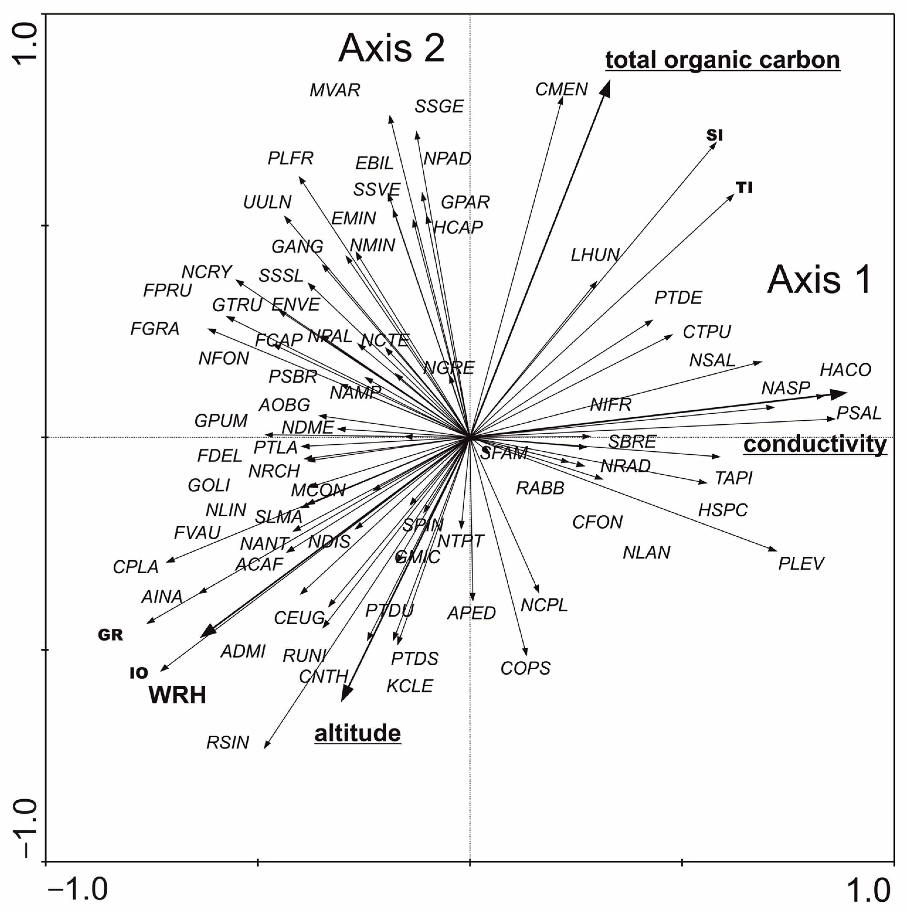
• Diatoms: The RDA analysis based on diatom taxa and environmental variables showed that the first two axes explained 28.5% of the variance in biological data and 71.7% of the variance in species–environment relationships. According to forward selection, conductivity, TOC, and altitude were the most strongly associated variables (statistically significant) with the distribution of diatom taxa and biotic metrics (Figure 6). Three distinct patterns were identified: (1) the distribution of Pleurosigma salinarum, Halamphora coffeaeformis, Navicula flandriae, N. salinarum var. salinarum, Pleurosira laevis var. laevis, Haslea spicula, N. lanceolata, and Surirella brebissonii was positively associated with conductivity; (2) Cyclotella meneghiniana, Lemnicola hungarica, and the values of SI and TI indices were positively correlated with TOC; (3) Amphora inariensis, Reimeria uniseriata, Cocconeis neothumensis, C. placentula var. placentula, C. euglypta, and the GR and IO index values were positively associated with altitude and WRH. The relationship between diatom composition and environmental variables was statistically significant (Monte Carlo test for the first canonical axis: p = 0.006, F = 2.071; for all canonical axes: p = 0.002, F = 1.810).
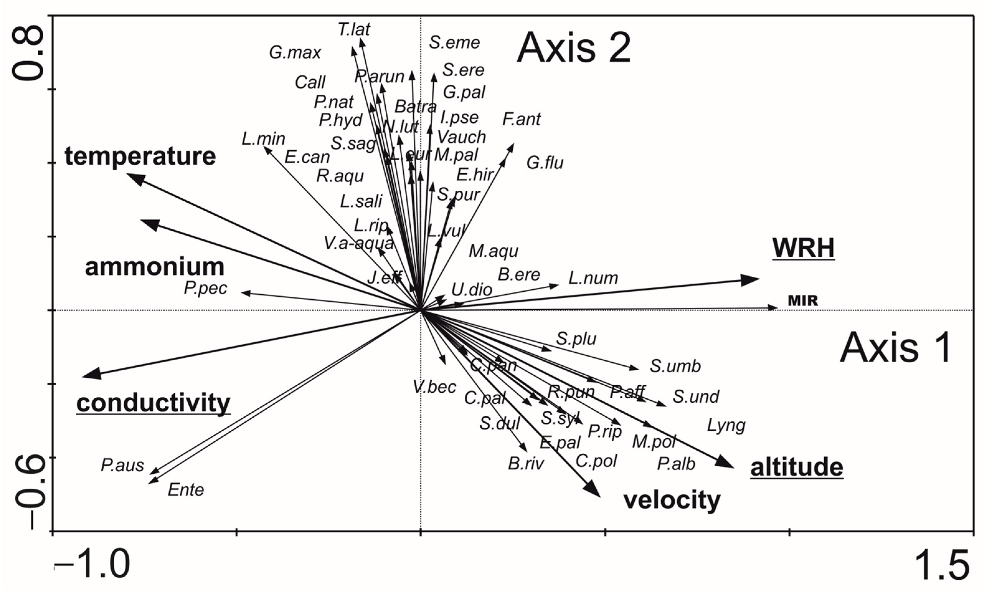
• Macrophytes: The first two axes explained 79.0% of the variance in biological data and 93.9% of the variance in species–environment relationships in RDA analysis (Figure 7). Based on forward selection, conductivity, altitude, and WRH were the variables most significantly associated with macrophyte distribution. Lyngbya sp., Scapania undulata, Brachythecium rivulare, Plagiomnium affine, Platyhypnidium riparioides, Chiloscyphus polyanthos, Marchantia polymorpha, Berula erecta, Ranunculus aquatilis, and the MIR index were positively correlated with flow velocity, altitude, and WRH. In contrast, conductivity influenced the distribution of Phragmites australis, Enteromorpha sp., and Potamogeton pectinatus most. The relationship between macrophyte composition and environmental variables was statistically significant (Monte Carlo test for the first canonical axis: p = 0.002, F = 26.179; for all axes: p = 0.002, F = 7.956).
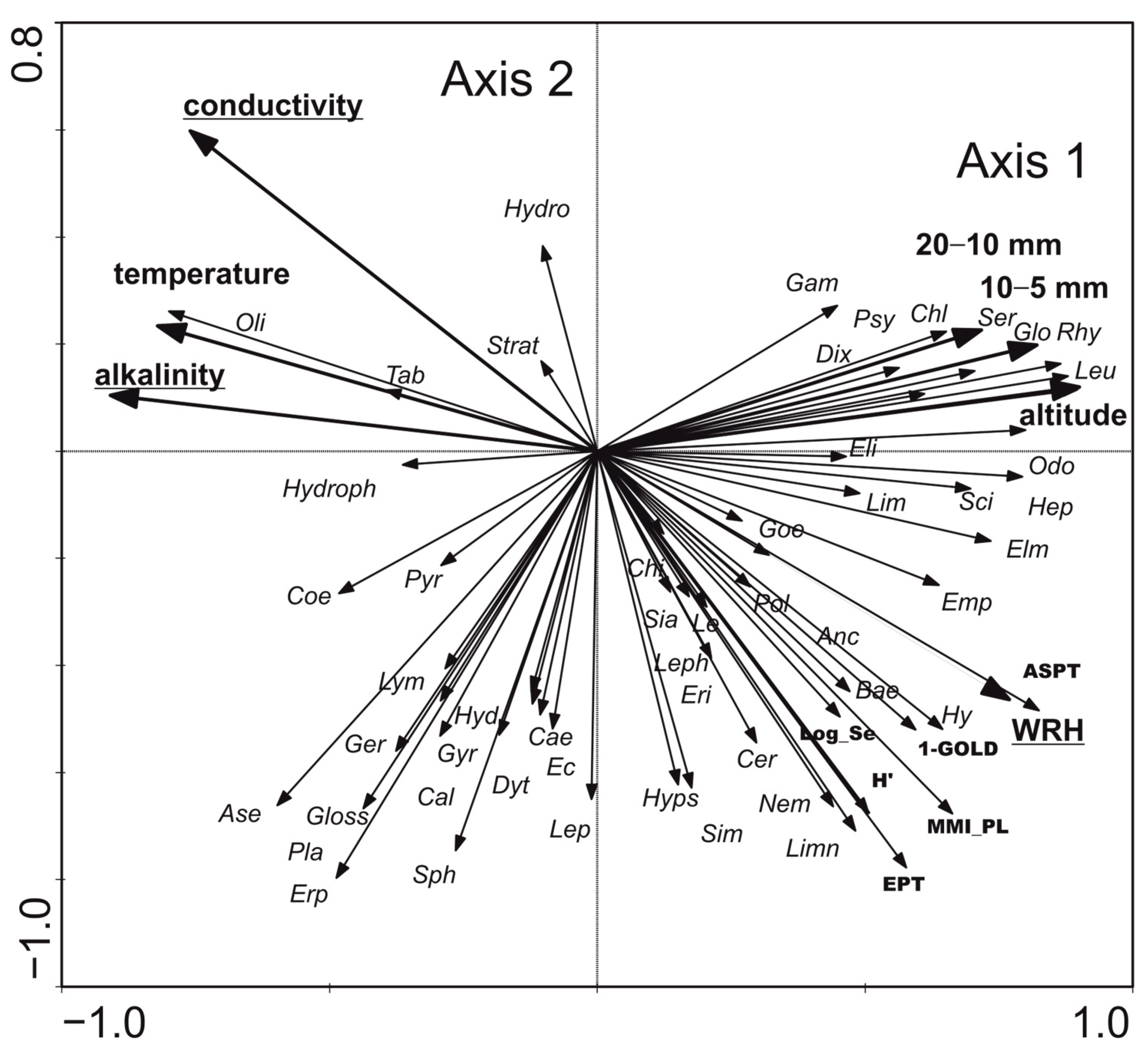
• Benthic macroinvertebrates: RDA showed that the first two axes explained 45.7% of the variance in biological data and 70.6% in species–environment relationships. Conductivity, alkalinity, and WRH were the most significant variables affecting macroinvertebrate distribution and biotic metrics (Figure 8). Three distribution patterns were established: (1) Hydrobiidae, Oligochaeta, Hydrophilidae, and Coenagrionidae were positively associated with higher conductivity, alkalinity, and temperature; (2) Gammaridae, Dixidae, Sericostomatidae, Glossosomatidae, Rhyacophilidae, and Odontoceridae were associated with altitude and coarse substrates (gravel and pebble); (3) the abundance of Ancylidae, Goeridae, Polycentropodidae, Lepidostomatidae, Limnephilidae, Chloroperlidae, Nemouridae, Leptophlebiidae, Baetidae, and Heptageniidae, along with high values of biotic metrics such as ASPT, 1-GOLD, H’, MMI_PL, and log₁₀(Sel_EPTD + 1), was positively correlated with WRH. The relationship was statistically significant (Monte Carlo test for the first axis: p = 0.002, F = 2.814; for all axes: p = 0.002, F = 2.103).
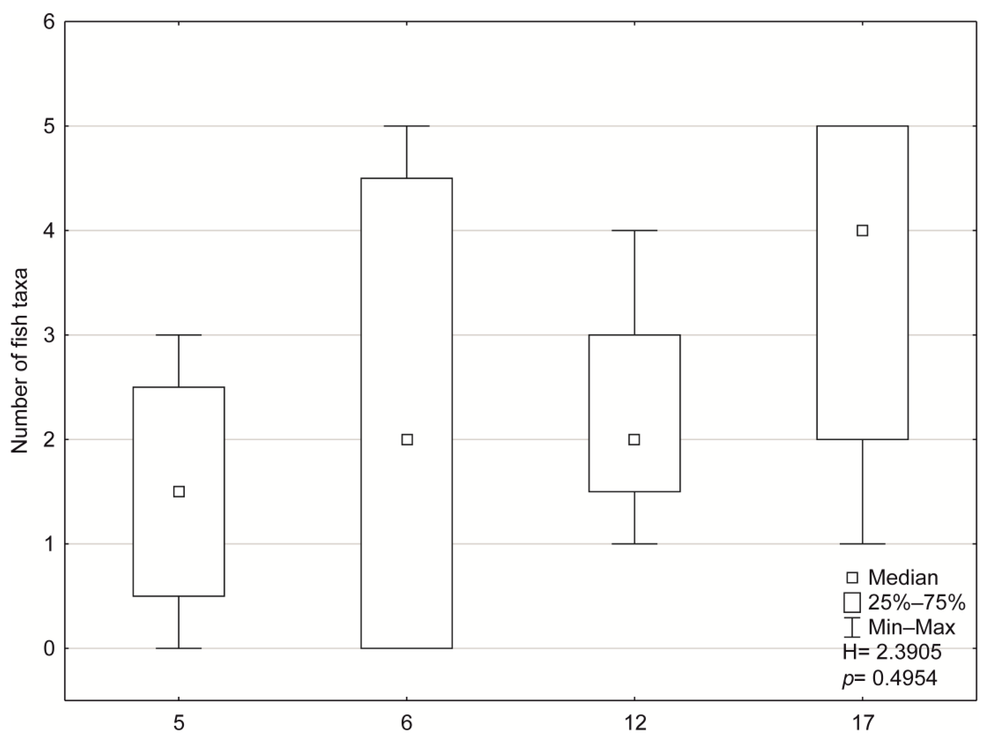
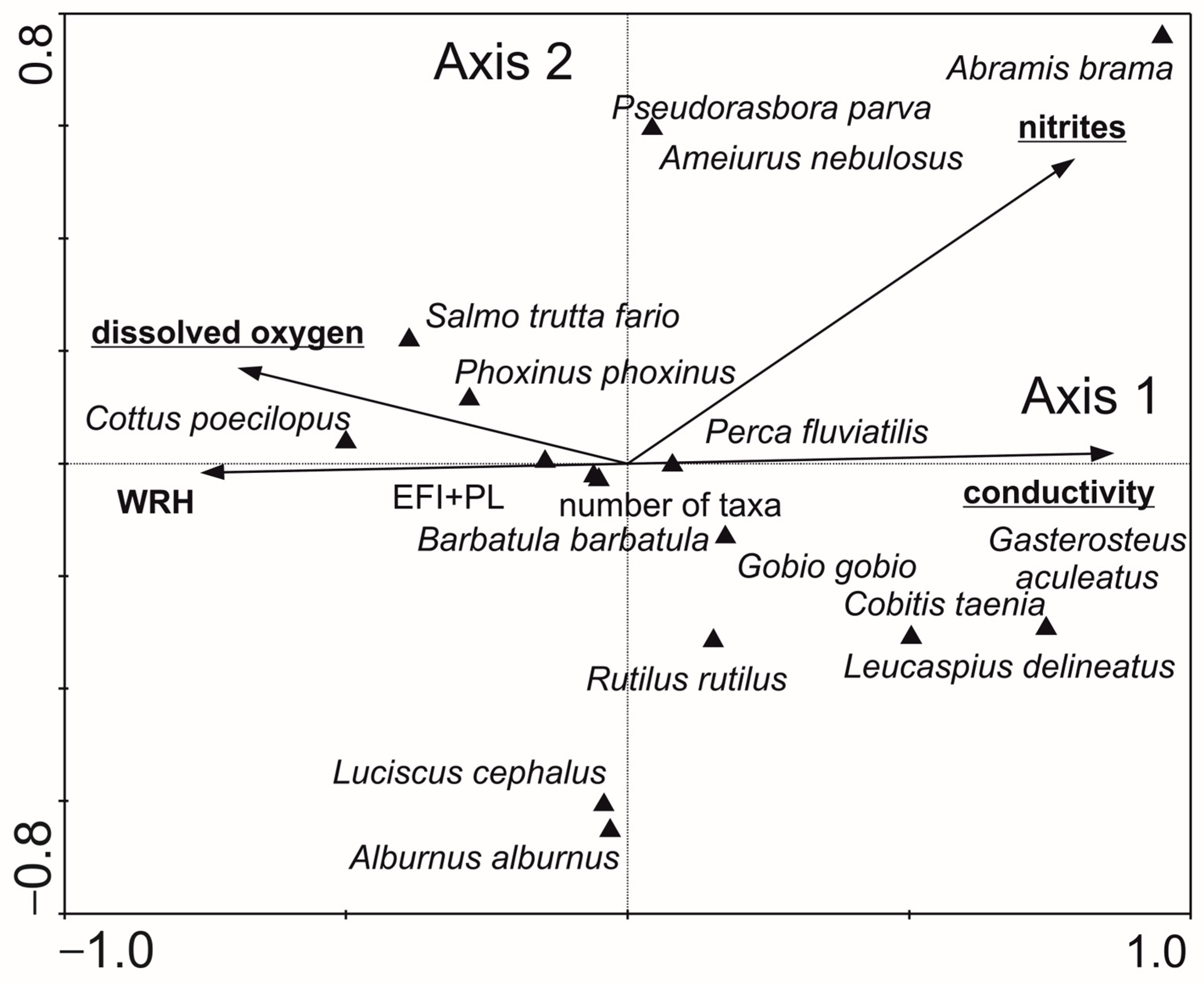
• Fish: The first two axes explained 32.1% of the variance in biological data and 72.9% in species–environment relationships in CCA analysis (Figure 9). Conductivity, dissolved oxygen, and nitrite concentration were the most significant variables. Gasterosteus aculeatus abundance was positively correlated with increasing conductivity. Salmo trutta fario, Phoxinus phoxinus, Cottus poecilopus, and Barbatula barbatula, as well as EFI + PL index values and total species number, were positively associated with a higher dissolved oxygen and WRH. The relationship between fish composition and environmental variables was statistically significant (Monte Carlo test for the first canonical axis: p = 0.006, F = 2.528; for all axes: p = 0.004, F = 2.165).

4. Discussion

4.1. Responses of Aquatic Organisms to Spatial and Anthropogenic Gradients

Our results demonstrate that the composition of aquatic communities and the values of biological indices were significantly shaped by both anthropogenic pressures and natural spatial gradients. Among the most influential stressors were increased salinity, nutrient enrichment, and hydromorphological degradation; natural variables such as altitude and flow velocity also modulated biological patterns. These findings are consistent with previous studies that emphasise the role of combined physicochemical and hydromorphological factors in structuring aquatic biota [10,11,25,46].

Salinity, closely linked to conductivity and chloride concentration, emerged as the most influential factor for all biological groups. Diatom communities exhibited marked shifts in species composition along this gradient, with salt-tolerant taxa such as Halamphora coffeaeformis, Navicula salinarum, and Pleurosira laevis var. laevis dominating in degraded sites with elevated salinity, particularly in the Bolina River, type 5 (up to 25.7 PSU). This observation is in line with earlier studies reporting the high sensitivity of diatom assemblages to salinisation [47,48,49] and corresponds with the documented effects of mine-derived saline water on planktonic communities in the Bolina River (type 5) [33]. Macrophytes also showed reduced diversity and compositional shifts in saline rivers, demonstrated the dominance of stress-tolerant taxa such as Phragmites australis and Enteromorpha sp. Benthic macroinvertebrates responded negatively to elevated salinity and nutrient levels, with the dominance of tolerant taxa such as Hydrobiidae, Oligochaeta, and Asellidae in degraded rivers. In contrast, reference-type rivers supported diverse assemblages including Baetidae, Heptageniidae, and Rhyacophilidae, which are sensitive to organic pollution and flow alteration. Similar patterns were reported by Lewin et al. [50] and Sowa et al. [51], who demonstrated sharp declines in macroinvertebrate richness along salinity and alkalinity gradients. These findings align with previous observations from the same river system, where saline mine waters reduced the diversity and structure of macroinvertebrate communities [34].

Fish assemblages, based on the EFI + PL index, showed a marked response to oxygen concentration and habitat quality. Salmo trutta fario, Phoxinus phoxinus, and Barbatula barbatula were associated with well-oxygenated, morphologically diverse habitats in flysch streams, whereas Gasterosteus aculeatus dominated in highly saline and degraded sites such as the Bolina River, type 5. Although previous studies (e.g., [52,53]) reported strong responses of fish to hydromorphological degradation, our findings suggest that in highly impacted systems, the effect of oxygen and salinity may override morphological influence.

The WRH index, which integrates hydromorphological quality, was significantly associated with community structure across all organism groups. Macrophytes and macroinvertebrates showed the strongest relationship, consistent with previous findings (e.g., [25,54,55]) and with studies showing the typology-specific responses of aquatic vegetation across Central European rivers [35]. Diatoms and fish also responded to WRH, although their sensitivity was partially masked by overriding chemical stressors. Shading, especially in forested flysch streams, may have reduced macrophyte abundance in some high-WRH sites, as suggested by Vermaat and Debruyne [56].

Altitude and stream gradient, as spatial variables, also explained part of the biological variation, particularly for diatoms and macrophytes. This aligns with previous findings show that altitude influences water temperature, flow dynamics, and substrate type, which in turn structure aquatic communities [24,57]. However, in our study, macroinvertebrates and fish showed limited sensitivity to altitude, possibly because salinity and low oxygen levels acted as overriding stressors that masked the effects of elevation.

Overall, our study confirms that individual BQEs differ in their sensitivity to specific environmental gradients. Diatoms and macroinvertebrates were most responsive to physical and chemical variables, while macrophytes and fish reflected hydromorphological conditions and spatial features. These patterns support previous meta-analyses that recommend the use of multimetric and multi-taxon approaches to detect stressor-specific responses in river systems [5,6,9].

4.2. Diagnostic Performance of Biological Indices Across Types of Rivers

The results demonstrate that the diagnostic performance of biological indices varied considerably across types of rivers, reflecting their differing sensitivity to specific stressors and environmental gradients. The strongest discrimination among types of rivers was achieved by IO and MMI_PL, both of which showed significant differences in values across all river categories (p < 0.01 and p < 0.03, respectively). The IO index exhibited the highest values in flysch rivers (type 12), with significantly lower values in anthropogenically modified rivers such as the Bolina and Mleczna rivers (types 5 and 6). The high sensitivity of diatom metrics to trophic and saprobic gradients [25,46,48] was visible, with low IO scores accompanied by elevated TI and SI values confirming the presence of nutrient and organic pollution. Moreover, the IO and GR indices were most responsive to changes in altitude and naturalness (WRH), whereas TI and SI were driven primarily by organic and nutrient enrichment. The MIR index also effectively differentiated between types of rivers (p < 0.001), with the highest values achieved in flysch streams and the lowest values achieved in degraded, saline rivers. In our study, this reflected not only eutrophication and nutrient stress, but also the effects of salinity and hydromorphological alteration, confirming macrophytes’ integrative reaction to both chemical and physical stressors [14,18,19]. Notably, the overall number of macrophyte taxa did not differ significantly among types of rivers, which suggests that metric values were driven more by compositional shifts than species richness alone. The MMI_PL index was especially effective in distinguishing degraded rivers from reference systems. The MMI_PL index was significantly lower in type 5 and 6 rivers, confirming its diagnostic strength in polluted, saline, and hydromorphologically modified conditions. Previous studies have demonstrated the reliability of macroinvertebrate-based multimetric indices in capturing both diffuse and point-source pollution as well as hydrological changes [6,25,50]. The EFI + PL index, though responsive to environmental gradients, was the least sensitive of the four indices to changes in water quality across types of rivers. Fish-based assessments showed a weaker gradient response, partly due to the low number of fish taxa recorded in degraded rivers and the strong overriding influence of oxygen levels. For instance, no fish were recorded in the Mleczna River (type 6), where oxygen levels were critically low. While fish indices are valuable indicators of long-term and catchment-scale pressures, their effectiveness may be constrained in small streams with limited species pools or acute oxygen depletion [10,53,58].

Overall, our results suggest that diatom and macroinvertebrate indices provided the most consistent and sensitive diagnostic tools across all types of rivers, particularly in detecting pollution gradients and distinguishing between natural and degraded conditions. Macrophyte indices were moderately effective, while fish-based indices were more variable and less robust under extreme physicochemical stress.

4.3. Typology-Specific Challenges in Ecological Assessment Under the WFD

The typology-based approach embedded in the WFD aims to account for natural variation in abiotic conditions among types of rivers when assessing ecological status [12]. However, our findings underscore several challenges that limit the effectiveness of this framework in practice.

First, the performance of biological indices varied markedly across types of rivers, despite being applied under standardised procedures. While diatom and macroinvertebrate indices provided the robust discrimination of anthropogenic impacts across all typological classes, fish- and macrophyte-based indices were less consistent, particularly in degraded or atypical systems. This inconsistency reflects the ecological limitations of some BQEs in specific types of rivers, especially under extreme salinisation or when biological communities show very low diversity. Our results align with earlier findings suggesting that biological indices often reflect stressor-specific or taxa-specific responses rather than a uniform signal across typologies [6,14,25].

Second, some biological responses were not strictly aligned with typological expectations. For example, the MIR index performed well in flysch rivers (type 12), but its values in lowland sandy rivers (type 17) varied despite the moderate pressure. The observed inconsistencies may result from the fact that abiotic typologies define natural expectations for biological communities, but anthropogenic pressures (e.g., salinity, morphological alteration, nutrient enrichment) can alter these communities in ways not easily predicted from typological categories alone. Recent studies suggest that trait-based or pressure-specific classification schemes may better explain biological variation than traditional typologies [28,29].

Third, although the WFD assumes the applicability of common reference conditions and class boundaries within each typological class, in reality, natural heterogeneity and uneven distribution of pressures complicate the establishment of true reference sites. Therefore, in many regions, reference conditions are approximated using the best available sites that exhibit minimal human impact. For instance, in our study, flysch rivers strong biological integrity, despite some hydromorphological modification, while lowland rivers were more affected by salinity and urban discharge. This highlights the practical challenges of defining and maintaining consistent reference conditions, especially in post-industrial landscapes [25,34].

Ultimately, while river typology remains a useful tool for setting expectations in ecological assessment, it may not provide sufficient diagnostic resolution when diverse and interacting pressures are present. Our findings indicate that typology-based classification could be improved by incorporating continuous environmental gradients such as conductivity or oxygenation and by integrating indices that are specific to particular stressors, as well as by expanding the use of multimetric and multi-taxa approaches [9,46]. Some of these concepts have already been implemented in national monitoring systems. For example, in France, the Macrophyte Biological Index for Rivers (IBMR) has been successfully applied across different river types and pollution intensities (nutrient enrichment and strong organic pollution) [59]. Applying such biologically responsive methods, in addition to typological classification, can enhance the diagnostic accuracy of ecological assessments, particularly in rivers affected by multiple or overlapping pressures (e.g., [60,61,62]).

4.4. Implications for Biomonitoring and Management Strategies

The findings of this study highlight key considerations for improving river biomonitoring and water management. The varying performance of biological indices across types of rivers suggests that monitoring strategies should be adapted to local abiotic conditions and dominant stressors. While multimetric indices such as MMI_PL and IO consistently detected degradation across typological classes, fish- and macrophyte-based assessments were more variable, particularly in lowland and saline rivers. This indicates that BQEs should be selected contextually, depending on their diagnostic relevance in a given setting. Benthic macroinvertebrates and diatoms demonstrated strong and consistent relationships with salinity, nutrient enrichment, and habitat quality, confirming their value as core bioindicators. These groups remain essential for integrated ecological classification, especially when used in combination. Although monitoring multiple BQEs increases the complexity and cost of assessments, their complementary responses to different stressors and time scales provide a more holistic picture of ecosystem condition [14,25]. Hydromorphological degradation emerged as a key factor structuring aquatic communities, particularly for fish and macrophytes. In our study, WRH index values were strongly linked to species composition and index variation, suggesting that management plans should place greater emphasis on physical habitat conditions. Moreover, the absence of fish in oxygen-poor sites illustrates the importance of recognising stressor-specific thresholds when interpreting biological results. This is especially relevant for rivers impacted by complex, interacting pressures where one dominant stressor may mask others. Improvements in future assessment frameworks may require us to adapt or refine river typology and reference conditions over time to reflect emerging pressures, environmental change, or improved ecological understanding. Incorporating continuous environmental gradients and trait-based metrics could enhance diagnostic resolution and better reflect ecological functioning. Our findings support the development of integrated, pressure-oriented monitoring strategies that maintain methodological consistency while accommodating regional and typological variability.

5. Conclusions

This study highlights the importance of integrating multiple BQEs and considering abiotic river typology when assessing ecological status under the WFD. Among the indices analysed, diatom and macroinvertebrate metrics proved most sensitive and consistent across typological classes, whereas fish and macrophyte indices were more variable and less effective in degraded rivers. Our results demonstrate that while the WFD’s typology-based framework is a valuable starting point, it may not fully capture the ecological consequences of complex and overlapping stressors such as salinisation, nutrient enrichment, and morphological alteration. Biological responses were shaped both by typological attributes and by local environmental gradients, particularly conductivity, oxygenation, and hydromorphological quality. The findings underscore the need for typology-aware, pressure-specific biomonitoring strategies that combine multiple organism groups and integrate continuous environmental variables. Such approaches can enhance the ecological realism and diagnostic accuracy of river assessment systems. At the same time, we acknowledge that the WFD was designed for harmonised application across the European Union, with the intercalibration process ensuring comparability between countries and river types. Balancing this need for standardisation with the goal of precise local diagnosis is a recognised challenge. The flexible application of BQEs across different spatial and temporal scales could help reconcile these objectives by maintaining consistency while allowing for site-specific ecological insights.

References

1. Dudgeon, D.; Arthington, A.H.; Gessner, M.O.; Kawabata, Z.; Knowler, D.J.; Lévêque, C.; Naiman, R.J.; Prieur-Richard, A.; Soto, D.; Stiassny, M.L.J.; et al. Freshwater biodiversity: Importance, threats, status and conservation challenges. Biol. Rev. 2006, 81, 163–182. [Google Scholar] [CrossRef] [PubMed]
2. Malmqvist, B.; Rundle, S. Threats to the running water ecosystems of the world. Environ. Conserv. 2002, 29, 134–153. [Google Scholar] [CrossRef]
3. Geist, J. Integrative freshwater ecology and biodiversity conservation. Ecol. Indic. 2011, 11, 1507–1516. [Google Scholar] [CrossRef]
4. Pont, D.; Hugueny, B.; Rogers, C. Development of a fish-based index for the assessment of river health in Europe: The European Fish Index. Fish. Manag. Ecol. 2007, 14, 427–439. [Google Scholar] [CrossRef]
5. Marzin, A.; Archaimbault, V.; Belliard, J.; Chauvin, C.; Delmas, F.; Pont, D. Ecological assessment of running waters: Do macrophytes, macroinvertebrates, diatoms and fish show similar responses to human pressures? Ecol. Indic. 2012, 23, 56–65. [Google Scholar] [CrossRef]
6. Birk, S.; Bonne, W.; Borja, A.; Brucet, S.; Courrat, A.; Poikane, S.; Solimini, A.; van de Bund, W.; Zampoukas, N.; Hering, D. Three hundred ways to assess Europe’s surface waters: An almost complete overview of biological methods to implement the Water Framework Directive. Ecol. Indic. 2012, 18, 31–41. [Google Scholar] [CrossRef]
7. Birk, S.; Chapman, D.; Carvalho, L.; Spears, B.M.; Andersen, H.E.; Argillier, C.; Auer, S.; Baattrup-Pedersen, A.; Banin, L.; Beklioğlu, M.; et al. Impacts of multiple stressors on freshwater biota across spatial scales and ecosystems. Nat. Ecol. Evol. 2020, 4, 1060–1068. [Google Scholar] [CrossRef]
8. Sabater, S.; Elosegi, A.; Ludwig, R. Multiple Stressors in River Ecosystems: Status, Impacts and Prospects for the Future; Elsevier: Amsterdam, The Netherlands, 2019; ISBN 9780128117132. [Google Scholar]
9. Lima, A.C.; Sayanda, D.; Wrona, F.J. A roadmap for multiple stressors assessment and management in freshwater ecosystems. Environ. Impact Assess. Rev. 2023, 102, 107191. [Google Scholar] [CrossRef]
10. Johnson, R.K.; Hering, D. Response of taxonomic groups in streams to gradients in resource and habitat characteristics. J. Appl. Ecol. 2009, 46, 175–186. [Google Scholar] [CrossRef]
11. Stubbington, R.; Sarremejane, R.; Laini, A.; Cid, N.; Csabai, Z.; England, J.; Munné, A.; Aspin, T.; Bonada, N.; Bruno, D.; et al. Disentangling responses to natural stressor and human impact gradients in river ecosystems across Europe. J. Appl. Ecol. 2022, 59, 537–548. [Google Scholar] [CrossRef]
12. European Commission. Directive 2000/60/EC of the European Parliament and of the Council—Establishing a Framework for Community Action in the Field of Water Policy; European Commission: Brussels, Belgium, 2000. [Google Scholar]
13. Poikane, S.; Salas Herrero, F.; Kelly, M.G.; Borja, A.; Birk, S.; van de Bund, W. European aquatic ecological assessment methods: A critical review of their sensitivity to key pressures. Sci. Total Environ. 2020, 740, 140075. [Google Scholar] [CrossRef]
14. Kolada, A.; Adamczyk, M.; Bielczyńska, A.; Bis, B.; Błachuta, J.; Błeńska, M.; Bociąg, K.; Brzeska-Roszczyk, P.; Ciecierska, H.; Dziemian, Ł.; et al. Handbook for the Biological Quality Elements (BQEs) Assessment and Ecological Status Classification of Surface Waters in Poland. Methodological Updating; Kolada, A., Ed.; Inspekcja Ochrony Środowiska: Warszawa, Poland, 2020; ISBN 978-83-950881-2-4. [Google Scholar]
15. Bis, B. Assessing the Ecological Status Assessment of Freshwaters. In Freshwater Ecosystems in Europe—An Educational Approach.Natural History Museum of Crete; Voreadou, C., Ed.; Selena Press: Heraklion, Greece, 2008; pp. 56–59. [Google Scholar]
16. Johnson, R.K.; Hering, D.; Furse, M.T.; Clarke, R.T. Detection of ecological change using multiple organism groups: Metrics and uncertainty. Hydrobiologia 2006, 566, 115–137. [Google Scholar] [CrossRef]
17. Zgrundo, A.; Peszek, Ł.; Poradowska, A. Manual for Monitoring and Evaluation of River Surface Water Bodies Based on Phytobenthos; Główny Inspektorat Ochrony Środowiska: Gdańsk, Poland, 2018.
18. Schneider, S. Macrophyte trophic indicator values from a European perspective. Limnologica 2007, 37, 281–289. [Google Scholar] [CrossRef]
19. Szoszkiewicz, K.; Zbierska, J.; Jusik, S.; Zgoła, T. Makrofitowa Metoda Oceny Rzek—Podręcznik Metodyczny Do Oceny i Klasyfikacji Stanu Ekologicznego Wód Płynących w Oparciu o Rośliny Wodne; Bogucki Wydawnictwo Naukowe: Poznań, Poland, 2010. [Google Scholar]
20. Rosenberg, D.M.; Resh, V.H. Freshwater Biomonitoring and Benthic Macroinvertebrates; Chapman and Hall: London, UK, 1993. [Google Scholar]
21. Bis, B.; Mikulec, A. Guide to Assess the Ecological Status of Rivers Based on Benthic Macroinvertebrate; Biblioteka Monitoringu Środowiska: Warszawa, Poland, 2013. [Google Scholar]
22. FAME CONSORTIUM Manual for the Application of the European Fish Index—EFI: A Fish-Based Method to Assess the Ecological Status of European Rivers in Support of the Water Framework Directive. Available online: https://pureportal.inbo.be/en/publications/manual-for-application-of-the-european-fish-index-efi-a-fish-base (accessed on 5 October 2019).
23. Prus, P.; Wiśniewolski, W.; Adamczyk, M. Monitoring of Riverine Ichthyofauna. Methodological Guide; Biblioteka Monitoringu Środowiska: Warszawa, Poland, 2016. [Google Scholar]
24. Szoszkiewicz, K.; Jusik, S.; Lewin, I.; Czerniawska-Kusza, I.; Kupiec, J.M.; Szostak, M. Macrophyte and macroinvertebrate patterns in unimpacted mountain rivers of two European ecoregions. Hydrobiologia 2018, 808, 327–342. [Google Scholar] [CrossRef]
25. Hering, D.; Johnson, R.K.; Kramm, S.; Schmuts, S.; Szoszkiewicz, K.; Verdonschot, P.F.M. Assessment of European streams with diatoms, macrophytes, macroinvertebrates and fish: A comparative metric-based analysis of organism response to stress. Freshw. Biol. 2006, 51, 1757–1785. [Google Scholar] [CrossRef]
26. Clarke, G.; Kernan, M.; Marchetto, A.; Sorvari, S.; Catalan, J. Using diatoms to assess geographical patterns of change in high-altitude European lakes from pre-industrial times to the present day. Aquat. Sci. 2005, 67, 224–236. [Google Scholar] [CrossRef]
27. Baattrup-Pedersen, A.; Szoszkiewicz, K.; Nijboer, R.; O’Hare, M.; Ferreira, T. Macrophyte communities in unimpacted European streams: Variability in assemblage patterns, abundance and diversity. Hydrobiologia 2006, 566, 179–196. [Google Scholar] [CrossRef]
28. Jusik, S.; Szoszkiewicz, K.; Kupiec, J.M.; Lewin, I.; Samecka-Cymerman, A. Development of comprehensive river typology based on macrophytes in the mountain-lowland gradient of different Central European ecoregions. Hydrobiologia 2015, 745, 241–262. [Google Scholar] [CrossRef]
29. Jupke, J.F.; Birk, S.; Álvarez-Cabria, M.; Aroviita, J.; Barquín, J.; Belmar, O.; Bonada, N.; Cañedo-Argüelles, M.; Chiriac, G.; Elexová, E.M.; et al. Evaluating the biological validity of European river typology systems with least disturbed benthic macroinvertebrate communities. Sci. Total Environ. 2022, 842, 156689. [Google Scholar] [CrossRef]
30. Szoszkiewicz, K.; Jusik, S.; Adynkiewicz-Piragas, M.; Gebler, D.; Achtenberg, K.; Radecki-Pawlik, A.; Okruszko, T.; Gielczewski, M.; Pietruczuk, K.; Przesmycki, M.; et al. Podręcznik Oceny Wód Płynących w Oparciu o Hydromorfologiczny Indeks Rzeczny; Biblioteka Monitoringu Środowiska: Warszawa, Poland, 2017. [Google Scholar]
31. Regulation of the Minister of the Environment of 22 July 2009 on the Classification of the Ecological Status, Ecological Potential and Chemical Status of Surface Water Bodies [Dz. U. 2009, Item 1018]. Available online: https://isap.sejm.gov.pl/isap.nsf/DocDetails.xsp?id=WDU20091221018 (accessed on 5 October 2019). (In Polish)
32. Regulation of the Minister of Infrastructure of 25 June 2021 on the Classification of Ecological Status, Ecological Potential and Chemical Status and the Method of Classifying the Status of Surface Water Bodies, as Well as Environmental Standards [Dz. U. 2021, Item 1475]. Available online: https://isap.sejm.gov.pl/isap.nsf/DocDetails.xsp?id=WDU20210001475 (accessed on 19 May 2025). (In Polish)
33. Halabowski, D.; Bielańska-Grajner, I.; Lewin, I. Effect of underground salty mine water on the rotifer communities in the Bolina River (Upper Silesia, Southern Poland). Knowl. Manag. Aquat. Ecosyst. 2019, 420, 31. [Google Scholar] [CrossRef]
34. Halabowski, D.; Lewin, I.; Buczyński, P.; Krodkiewska, M.; Płaska, W.; Sowa, A.; Buczyńska, E. Impact of the Discharge of Salinised Coal Mine Waters on the Structure of the Macroinvertebrate Communities in an Urban River (Central Europe). Water Air Soil Pollut. 2020, 231, 5. [Google Scholar] [CrossRef]
35. Halabowski, D.; Lewin, I. Impact of anthropogenic transformations on the vegetation of selected abiotic types of rivers in two ecoregions (Southern Poland). Knowl. Manag. Aquat. Ecosyst. 2020, 421, 35. [Google Scholar] [CrossRef]
36. Halabowski, D.; Lewin, I. Triggers for the Impoverishment of the Macroinvertebrate Communities in the Human-Impacted Rivers of Two Central European Ecoregions. Water Air Soil Pollut. 2021, 232, 55. [Google Scholar] [CrossRef]
37. Halabowski, D.; Bielańska-Grajner, I.; Lewin, I.; Sowa, A. Diversity of Rotifers in Small Rivers Affected by Human Activity. Diversity 2022, 14, 127. [Google Scholar] [CrossRef]
38. Myślińska, E. Organic and Laboratory Land Testing Methods; Państwowe Wydawnictwo Naukowe: Warszawa, Poland, 2001. [Google Scholar]
39. Hermanowicz, W.; Dojlido, J.; Dożańska, W.; Koziorowski, B.; Zerbe, J. Physical and Chemical Studies of Water and Wastewater; Arkady: Warszawa, Poland, 1999. [Google Scholar]
40. Szoszkiewicz, K.; Jusik, S.; Gebler, D.; Achtenberg, K.; Adynkiewicz-Piragas, M.; Artur Radecki-Pawlik, A.; Okruszko, T.; Pietruczuk, K.; Przesmycki, M.; Nawrocki, P. Hydromorphological Index for Rivers: A New Method for Hydromorphological Assessment and Classification for Flowing Waters in Poland. J. Ecol. Eng. 2020, 21, 261–271. [Google Scholar] [CrossRef]
41. Picińska-Fałtynowicz, J.; Błachuta, J.; Kotowicz, J.; Mazurek, M.; Rawa, W. Select the Types of Water Bodies River and Lake to Assess the Ecological Status Based on Phytobenthos with the Recommendation of the Methodology of Collection and Analysis of Samples; Główny Inspektorat Ochrony Środowiska: Wrocław, Poland, 2006.
42. Picińska-Fałtynowicz, J.; Błachuta, J. A Practical Guide: Sampling, Preparation and Processing of Diatom Phytobenthos Residing in Rivers and Lakes; Instytut Meteorologii i Gospodarki Wodnej: Wrocław, Poland, 2010. [Google Scholar]
43. ISO 10870:2012; Water Quality—Guidelines for the Selection of Sampling Methods and Devices for Benthic Macroinvertebrates in Fresh Waters. Available online: https://www.iso.org/standard/46251.html (accessed on 19 May 2025).
44. Ter Braak, C.J.F.; Šmilauer, P. CANOCO Reference Manual and CanoDraw for Windows User’s Guide: Software for Canonical Community Ordination (Version 4.5), 2nd ed.; Microcomputer Power: New York, NY, USA, 2002. [Google Scholar]
45. McCune, B.; Grace, J.B. Analysis of Ecological Communities; MjM Software Design: Gleneden Beach, OR, USA, 2002. [Google Scholar]
46. Morin, S.; Gómez, N.; Tornés, E.; Licursi, M.; Rosebery, J. Benthic Diatom Monitoring and Assessment of Freshwater Environments: Standard Methods and Future Challenges. In Aquatic Biofilms: Ecology, Water Quality and Wastewater Treatment; Romaní, A.M., Guasch, H., Balaguer, M.D., Eds.; Caister Academic Press: Wymondham, UK, 2016; pp. 111–124. [Google Scholar]
47. Herbert, E.R.; Boon, P.; Burgin, A.J.; Neubauer, S.C.; Franklin, R.B.; Ardón, M.; Hopfensperger, K.N.; Lamers, L.P.M.; Gell, P. A global perspective on wetland salinization: Ecological consequences of a growing threat to freshwater wetlands. Ecosphere 2015, 6, 206. [Google Scholar] [CrossRef]
48. Bąk, M.; Halabowski, D.; Kryk, A.; Lewin, I.; Sowa, A. Mining salinisation of rivers: Its impact on diatom (Bacillariophyta) assemblages. Fottea 2020, 20, 1–16. [Google Scholar] [CrossRef]
49. Chen, K.; Sun, D.; Rajper, A.R.; Mulatibieke, M.; Hughes, R.M.; Pan, Y.; Tayibazaer, A.; Chen, Q.; Wang, B. Concordance in biological condition and biodiversity between diatom and macroinvertebrate assemblages in Chinese arid-zone streams. Hydrobiologia 2019, 829, 245–263. [Google Scholar] [CrossRef]
50. Lewin, I.; Jusik, S.; Szoszkiewicz, K.; Czerniawska-Kusza, I.; Ławniczak, A.E. Application of the new multimetric MMI_PL index for biological water quality assessment in reference and human-impacted streams (Poland, the Slovak Republic). Limnologica 2014, 49, 42–51. [Google Scholar] [CrossRef]
51. Sowa, A.; Krodkiewska, M.; Halabowski, D.; Lewin, I. Response of the mollusc communities to environmental factors along an anthropogenic salinity gradient. Sci. Nat. 2019, 106, 60. [Google Scholar] [CrossRef]
52. Gorman, O.T.; Karr, J.R. Habitat Structure and Stream Fish Communities. Ecology 1978, 59, 507–515. [Google Scholar] [CrossRef]
53. Przybylski, M.; Głowacki, Ł.; Grabowska, J.; Kaczkowski, Z.; Kruk, A.; Marszał, L.; Zięba, G.; Ziułkiewicz, M. Riverine Fish Fauna in Poland. In Polish River Basins and Lakes—Part II. The Handbook of Environmental Chemistry; Korzeniewska, E., Harnisz, M., Eds.; Springer: Cham, Switzerland, 2020; pp. 195–238. [Google Scholar]
54. Buffagni, A.; Erba, S.; Cazzola, M.; Kemp, J.L. The AQEM multimetric system for the southern Italian Apennines: Assessing the impact of water quality and habitat degradation on pool macroinvertebrates in Mediterranean rivers. Hydrobiologia 2004, 516, 313–329. [Google Scholar] [CrossRef]
55. Lewin, I.; Czerniawska-Kusza, I.; Szoszkiewicz, K.; Ławniczak, A.E.; Jusik, S. Biological indices applied to benthic macroinvertebrates at reference conditions of mountain streams in two ecoregions (Poland, the Slovak Republic). Hydrobiologia 2013, 709, 183–200. [Google Scholar] [CrossRef]
56. Vermaat, J.E.; De Bruyne, R.J. Factors limiting the distribution of submerged waterplants in the lowland River Vecht (The Netherlands). Freshw. Biol. 1993, 30, 147–157. [Google Scholar] [CrossRef]
57. Šporka, F.; Pastuchová, Z.; Hamerlík, L.; Dobiašová, M.; Beracko, P. Assessment of running waters (Slovakia) using benthic macroinvertebrates—Derivation of ecological quality classes with respect to altitudinal gradients. Biologia 2009, 64, 1196–1205. [Google Scholar] [CrossRef]
58. Hughes, S.J.; Santos, J.M.; Ferreira, M.T.; Caraça, R.; Mendes, A.M. Ecological assessment of an intermittent Mediterranean river using community structure and function: Evaluating the role of different organism groups. Freshw. Biol. 2009, 54, 2383–2400. [Google Scholar] [CrossRef]
59. Haury, J.; Peltre, M.-C.; Trémolières, M.; Barbe, J.; Thiébaut, G.; Bernez, I.; Daniel, H.; Chatenet, P.; Haan-Archipof, G.; Muller, S.; et al. A new method to assess water trophy and organic pollution—The Macrophyte Biological Index for Rivers (IBMR): Its application to different types of river and pollution. Macrophytes Aquat. Ecosyst. Biol. Manag. 2006, 190, 153–158. [Google Scholar]
60. Theodoropoulos, C.; Karaouzas, I.; Vourka, A.; Skoulikidis, N. ELF—A benthic macroinvertebrate multi-metric index for the assessment and classification of hydrological alteration in rivers. Ecol. Indic. 2020, 108, 105713. [Google Scholar] [CrossRef]
61. Feio, M.J.; Hughes, R.M.; Callisto, M.; Nichols, S.J.; Odume, O.N.; Quintella, B.R.; Kuemmerlen, M.; Aguiar, F.C.; Almeida, S.F.P.; Alonso-EguíaLis, P.; et al. The Biological Assessment and Rehabilitation of the World’s Rivers: An Overview. Water 2021, 13, 371. [Google Scholar] [CrossRef]
62. Assefa, W.W.; Eneyew, B.G.; Wondie, A. Development of a multi-metric index based on macroinvertebrates for wetland ecosystem health assessment in predominantly agricultural landscapes, Upper Blue Nile basin, northwestern Ethiopia. Front. Environ. Sci. 2023, 11, 1117190. [Google Scholar] [CrossRef]
Figure 1. Values of indices of the ecological status of (A) diatoms (IO), (B) macrophytes (MIR), (C) benthic macroinvertebrates (MMI_PL) and (D) fish (EFI + PL) in abiotic types of rivers. * Asterisks above a whisker denote significant differences between abiotic types of rivers (5, 6, 12, 17).
Water 17 01817 g001
Figure 2. Number of diatom taxa (A,B) values of trophic index (TI), (C) saprobic index (SI), and (D) reference taxa abundance index (GR). * Asterisks above a whisker denote significant differences between abiotic types of rivers (5, 6, 12, 17).
Water 17 01817 g002
Figure 3. Number of macrophyte taxa among abiotic types of rivers (5, 6, 12, 17).
Water 17 01817 g003
Figure 4. Values of components of the Polish multimetric index for macroinvertebrates (MMI_PL) for the abiotic types of rivers (5, 6, 12, 17). * Asterisks above a whisker denote significant differences between the abiotic types of rivers. Abbreviations: (A) EPT index—the total number of families in the Ephemeroptera, Plecoptera and Trichoptera taxa; (B) H′—Shannon–Wiener index; (C) the number of benthic macroinvertebrate taxa; (D) ASPT index—Average Score per Taxon; (E) 1-GOLD index—the relative abundance of Gastropoda, Oligochaeta and Diptera; (F) Log10(Sel_EPTD + 1) − index log10 (sum of individuals of the families Heptageniidae, Ephemeridae, Leptophlebiidae, Brachycentridae, Georidae, Polycentropodidae, Limnephilidae, Odontoceridae, Dolichopodidae, Stratiomyidae, Dixidae, Empididae, Athericidae, Nemouridae + 1).
Water 17 01817 g004
Figure 5. Number of fish taxa among abiotic types of rivers (5, 6, 12, 17).
Water 17 01817 g005
Figure 6. Ordination diagram (biplot) based on redundancy analysis (RDA) of diatom taxa, biotic metrics, and selected environmental variables (statistically significant environmental variables are underlined). Abbreviations: ACAF—Achnanthidium affine, ADMI—Achnanthidium minutissimum, AINA—Amphora inariensis, AOBG—Platessa oblongella, APED—Amphora pediculus, CEUG—Cocconeis euglypta, CFON—Caloneis fontinalis, CMEN—Cyclotella meneghiniana, CNTH—Cocconeis neothumensis, COPS—Cocconeis pseudothumensis, CPLA—Cocconeis placentula, CTPU—Ctenophora pulchella, EBIL—Eunotia bilunaris, EMIN—Eunotia minor, ENVE—Encyonema ventricosum, FCAP—Fragilaria capucina, FDEL—Fragilaria predelicatissima, FGRA—Fragilaria gracilis, FPRU—Fragilaria pararumpens, FVAU—Fragilaria vaucheriae, GANG—Gomphonema angustatum, GMIC—Gomphonema micropus, GOLI—Gomphonema olivaceum, GPAR—Gomphonema parvulum, GPUM—Gomphonema pumilum, GTRU—Gomphonema truncatum, HACO—Halamphora coffeaeformis, HCAP—Hippodonta capitate, HSPC—Haslea spicula, KCLE—Karayevia clevei, LHUN—Lemnicola hungarica, MCON—Meridion constrictum, MVAR—Melosira varians, NAMP—Nitzschia amphibia, NANT—Navicula antonii, NASP—Navicula flandriae, NCPL—Nitzschia capitellata, NCRY—Navicula cryptocephala, NCTE—Navicula cryptotenella, NDIS—Nitzschia dissipata, NDME—Nitzschia dissipata var. media, NFON—Nitzschia fonticola, NGRE—Navicula gregaria, NIFR—Nitzschia frustulum, NLAN—Navicula lanceolate, NLIN—Nitzschia linearis, NMIN—Navicula minima, NPAD—Nitzschia palea var. debilis, NPAL—Nitzschia palea var. palea, NRAD—Navicula radiosa, NRCH—Navicula reichardtiana, NSAL—Navicula salinarum var. salinarum, NTPT—Navicula tripunctata, PLEV—Pleurosira laevis var. laevis, PLFR—Planothidium frequentissimum, PSAL—Pleurosigma salinarum, PSBR—Pseudostaurosira brevistriata, PTDE—Planothidium delicatulum, PTDS—Planothidium nanum, PTDU—Planothidium dubium, PTLA—Planothidium lanceolatum, RABB—Rhoicosphenia abbreviate, RSIN—Reimeria sinuate, RUNI—Reimeria uniseriata, SBRE—Surirella brebissonii, SFAM—Synedra famelica, SLMA—Staurosirella martyi, SPIN—Staurosirella pinnata, SSGE—Sellaphora saugerresii, SSSL—Staurosira subsalina, SSVE—Staurosira venter, TAPI—Tryblionella apiculata, UULN—Ulnaria ulna, IO—multimetric diatom index, TI—trophic index, SI—saprobic index, GR—reference taxa abundance index, WRH—Hydromorphological Diversity Index.
Water 17 01817 g006
Figure 7. Ordination diagram (biplot) based on redundancy analysis (RDA) of macrophyte species, biotic metrics, and selected environmental variables (statistically significant environmental variables are underlined). Abbreviations: B.ere—Berula erecta, B.riv—Brachythecium rivulare, Batra—Batrachyspermum sp., C.pal—Caltha palustris, C.pan—Carex paniculata, C.pol—Cochlearia polonica, Call—Callitriche sp., E.can—Elodea canadensis, E.hir—Epilobium hirsutum, E.pal—Equisetum palustre, Ente—Enteromorpha sp., F.ant—Fontinalis antipyretica, G.flu—Glyceria fluitans, G.max—Glyceria maxima, G.pal—Galium palustre, I.pse—Iris pseudoacorus, J.eff—Juncus effusus, L.eur—Lycopus europaeus, L.min—Lemna minor, L.num—Lysimachia nummularia, L.rip—Leptodictyum riparium, L.sali—Lythrum salicaria, L.vul—Lysimachia vulgaris, Lyng—Lyngbya sp., M.aqu—Mentha aquatica, M.pal—Myosotis palustris, M.pol—Marchantia polymorpha, N.lut—Nuphar lutea, P.aff—Plagiomnium affine, P.alb—Petasites albus, P.arun—Phalaris arundinacea, P.aus—Phragmites australis, P.hyd—Polygonum hydropiper, P.nat—Potamogeton natans, P.pec—Potamogeton pectinatus, P.rip—Platyhypnidium riparioides, R.aqu—Ranunculus aquatilis, R.pun—Rhizomnium punctatum, S.dul—Solanum dulcamara, S.eme—Sparganium emersum, S.ere—Sparganium erectum, S.plu—Sciuro-hypnum plumosum, S.pur—Salix purpurea, S.sag—Sagittaria sagittifolia, S.syl—Scirpus sylvaticus, S.umb—Scrophularia umbrosa, S.und—Scapania undulata, T.lat—Typha latifolia, U.dio—Urtica dioica, V.a-aqua—Veronica anagallis-aquatica, V.bec—Veronica beccabunga, Vauch—Vaucheria sp., WRH—Hydromorphological Diversity Index, MIR—Macrophyte Index for Rivers.
Water 17 01817 g007
Figure 8. Ordination diagram (biplot) based on redundancy analysis (RDA) of benthic macroinvertebrate taxa, biotic metrics, and selected environmental variables (statistically significant environmental variables are underlined). Abbreviations: Anc—Ancylidae; Ase—Asellidae; Bae—Baetidae; Cae—Caenidae; Cal—Calopterigidae; Cer—Ceratopogonidae; Chi—Chironomidae; Chl—Chloroperlidae; Coe—Coenagrionidae; Dix—Dixidae; Dyt—Dytiscidae; Ec—Ecnomidae; Elm—Elmidae; Emp—Empididae; Eli—Ephemerellidae; Eri—Ephemeridae; Erp—Erpobdellidae; Gam—Gammaridae; Ger—Gerridae; Gloss—Glossiphonidae; Glo—Glossosomatidae; Goe—Goeridae; Gyr—Gyrynidae; Hep—Heptageniidae; Hy—Hydrachnida; Hydro—Hydrobiidae; Hydroph—Hydrophilidae; Hyps—Hydropsychidae; Hyd—Hydroptilidae; Le—Lepidostomatidae; Lep—Leptoceridae; Leph—Leptophlebidae; Leu—Leuctridae; Limn—Limnephilidae; Lim—Limonidae; Lym—Lymnaeidae; Nem—Nemouridae; Odo—Odontoceridae; Oli—Oligochaeta; Pla—Planorbidae; Pol—Polycentropodidae; Psy—Psychodidae; Pyr—Pyralidae; Rhy—Rhyacophilidae; Sci—Scirtidae; Ser—Sericostomatidae; Sia—Sialidae; Sim—Simuliidae; Sph—Sphaeriidae; Strat—Stratiomyidae; Tab—Tabanidae; 5–10, 10–20 mm—coarse substrates (gravel and pebble); WRH—Hydromorphological Diversity Index; MMI_PL—multimetric index for macroinvertebrates; MMI_PL: EPT—total number of families in the Ephemeroptera, Plecoptera and Trichoptera taxa; H’—Shannon–Wiener index; ASPT—Average Score per Taxon; Log_Se—log10 of sum of selected families.
Water 17 01817 g008
Figure 9. Ordination diagram (biplot) based on canonical correspondence analysis (CCA) of fish species, biotic metrics, and selected environmental variables (statistically significant environmental variables are underlined). Abbreviations: WRH—Hydromorphological Diversity Index.
Water 17 01817 g009