AI-Driven Time Series Forecasting of Coastal Water Quality Using Sentinel-2 Imagery: A Case Study in the Gulf of Thailand

Abstract

The accurate prediction of water quality parameters is essential for effective pollution control and resource management. This study presents a hybrid AI-remote sensing framework for forecasting water quality in the Gulf of Thailand, which combines Sentinel-2 imagery with Support Vector Machine (SVM) and Autoregressive Integrated Moving Average (ARIMA) models. Our approach achieves a 5.4× increase in data coverage over traditional methods, demonstrating the effectiveness of machine learning in environmental monitoring. Predictive accuracy was evaluated across Support Vector Machine (SVM), ARIMA, and Amazon Forecast models. Results indicate that SVM, optimised through RBF kernel and grid search, outperforms other models for Chlorophyll-a (RMSE: 1.8), while ARIMA exhibits superior performance for Secchi Depth (RMSE: 0.2) and Trophic State Index (RMSE: 0.8). The study also introduces Aqua Sight, a web-based visualisation tool built on Google Earth Engine, enabling stakeholders to access real-time water quality forecasts. These findings highlight the potential of integrating satellite-derived data with machine learning to enhance early warning systems and support environmental decision making in coastal ecosystems.

1. Introduction

Water quality monitoring is fundamental to marine ecosystem management and is crucial for safeguarding biodiversity and supporting marine-dependent economies. This assertion is particularly relevant in regions such as the Gulf of Thailand, where significant pressures from rapid industrialisation, urban expansion, increased maritime traffic, and climate change-related disturbances have led to elevated pollution levels, habitat degradation, and shifts in oceanographic conditions [1,2]. Such conditions emphasise the need for robust water quality assessments, particularly concerning key indicators, such as chlorophyll-a concentration, which is a primary metric for assessing phytoplankton biomass and overall primary productivity in these waters [3,4].

In the Gulf of Thailand, chlorophyll-a serves as a vital indicator of eutrophication and algal biomass, influenced by nutrient inputs from agricultural runoff and wastewater discharge [5,6]. For example, studies have demonstrated chlorophyll-a’s capacity to effectively indicate the eutrophication process, where nutrient loadings directly affect its concentration in water bodies [7]. Similarly, turbidity reflects suspended sediments, affecting light penetration and phytoplankton growth [8,9], while dissolved oxygen (DO) fluctuations can lead to hypoxic conditions [10,11]. Monitoring nutrient levels, particularly nitrogen and phosphorus, as well as parameters such as chlorophyll-a and turbidity, is crucial for mitigating these risks and maintaining the health of marine ecosystems [12,13]. Overall, the interrelationship of these factors underscores the importance of a comprehensive water quality monitoring system. Such systems provide real-time data necessary for addressing current ecological challenges and play an instrumental role in making informed management decisions that foster the sustainability of marine resources in vulnerable regions, such as the Gulf of Thailand [14,15].

The ecological and economic significance of maintaining optimal water quality in the Gulf of Thailand is profound, as it supports marine biodiversity and coastal livelihoods. Effective monitoring and forecasting of water quality parameters are essential to mitigate environmental degradation. However, while precise, traditional in situ sampling methods require extensive resources and yield spatially limited data [16,17]. Conventional techniques yield data points that are spatially and temporally constrained; they primarily reflect localised conditions rather than broader ecological shifts occurring in the marine context. For instance, the seasonal variations influenced by monsoonal patterns significantly affect water quality in the Gulf [18]. These variations necessitate frequent data collection, which becomes logistically challenging, particularly in remote offshore regions. This underscores the need to drive innovation by combining remote sensing and machine learning [19,20].

Integrating remote sensing technologies with machine learning algorithms presents a promising solution to overcome these limitations. Remote sensing enables continuous, large-scale monitoring, while machine learning facilitates the real-time analysis of these datasets [16,19]. Techniques such as time series analysis effectively extract patterns from historical environmental data, enabling timely predictions of water quality changes—critical in dynamic marine settings, such as the Gulf of Thailand [21,22].

This study aims to develop and evaluate machine learning-based time series forecasting models for predicting key water quality parameters in the Gulf of Thailand using high-resolution Sentinel-2 remote sensing data. Specifically, we carry out the following:

I.

Investigate the performance of hybrid approaches combining deep learning, tree-based ensembles, and classical statistical models.

II.

Address critical gaps in existing coastal water quality forecasting.

The following key research gaps are addressed:

I.

Limited use of Sentinel-2’s 10 m resolution data for tropical coastal waters (vs. MODIS/Landsat in prior works [16,22].

II.

Lack of systematic comparison between ARIMA and modern ML (SVM, LSTM) for water quality parameters [23,24].

III.

An operational disconnect between models and stakeholder tools [25,26].

The study makes the following novel contributions:

I.

First multi-model benchmarking framework for Gulf of Thailand water quality;

II.

Aqua Sight platform bridges forecasts to real-world decision making;

III.

Data coverage increased by 5.4× via Sentinel-2/in situ fusion.

To ensure methodological clarity and to establish a strong scientific basis for our analysis, this study is guided by the following research objectives and hypotheses:

Research Objectives:

I.

To evaluate the feasibility and effectiveness of using satellite remote sensing data to forecast key water quality indicators—Chlorophyll-a, Secchi Depth, and Trophic State Index—in coastal marine environments;

II.

To compare the predictive accuracy of multiple time series forecasting models, including traditional statistical approaches (e.g., ARIMA) and advanced machine learning algorithms (e.g., SVM, Amazon Forecast, and ensemble methods);

III.

To explore the spatiotemporal variability in water quality parameters across monitoring stations within the Gulf of Thailand.

Research Hypotheses:

I.

H1: Support Vector Machine (SVM) models, particularly when optimised using RBF kernel and grid search, will yield superior accuracy in forecasting nonlinear water quality parameters, such as Chlorophyll-a.

II.

H2: ARIMA models will provide better forecasts for parameters showing seasonal linear patterns, such as Secchi Depth and Trophic State Index.

III.

H3: Integrating remotely sensed data with in situ measurements will enhance forecasting accuracy compared to using either data source in isolation.

These hypotheses are evaluated using standard performance metrics, including Mean Absolute Error (MAE), Root Mean Square Error (RMSE), and Mean Absolute Scaled Error (MASE), across various spatial locations and temporal intervals.

2. Related Works

Machine learning applications in environmental monitoring are rapidly advancing [23,27], with numerous studies demonstrating their effectiveness in predicting water quality indices using various algorithms adept at managing the complexities of aquatic datasets [24,28]. Adaptive, integrative approaches combining remote sensing and advanced computational techniques hold substantial promise for enhancing the efficiency and effectiveness of water quality management practices in the Gulf of Thailand and similar marine ecosystems worldwide [19,25,28].

Recent advancements in machine learning, particularly deep learning architectures, such as recurrent neural networks (RNNs) and long short-term memory (LSTM) networks, have shown exceptional predictive accuracy in time series forecasting applications, including water quality estimation. These models effectively capture complex temporal relationships within historical datasets, enabling them to project future water quality conditions. For instance, Bounoua et al. highlight the effectiveness of deep learning models, such as ConvLSTM and CNN-LSTM, in managing the intricate spatiotemporal patterns inherent in remote sensing data [29]. Additionally, hybrid approaches that integrate statistical models with deep learning, such as LSTM, have significantly enhanced predictive performance in dynamic environmental data scenarios [30].

Moreover, integrating machine learning techniques with remote sensing data further enhances forecasting capabilities by leveraging multiple sources of information. This includes critical variables, such as sea surface temperature, ocean colour indices, and meteorological data, collectively improving model robustness and generalisation [26]. For example, Chen et al. discuss the challenges and prospects of utilising big data from remote sensing for effective water environment monitoring, underscoring the vital role of innovative machine learning methods in data modelling and analysis [26]. Studies have demonstrated that using remote sensing in conjunction with machine learning can substantially improve water quality parameters, facilitating timely and impactful environmental observations [31,32].

Investigations into the application of machine learning for water quality assessment have consistently yielded promising outcomes. Zhou and Zhang emphasise the transformative potential of machine learning models in integrating remote sensing data for effective monitoring and prediction of water quality, particularly in challenging environments, such as Erhai Lake [20]. Moreover, research by Wu et al. suggests that ensemble learning techniques can enhance the accuracy of water quality estimations derived from satellite imagery [33]. Recent advances align closely with our research objectives. First, ARIMA’s effectiveness for seasonal parameters, such as Secchi Depth (Objective II), was demonstrated in tropical estuaries by Laosuwan et al. [16] (supporting H2). Second, SVM-RBF’s superiority for chlorophyll-a forecasting (Objective II/H1) echoes findings from Zheng et al. [34] in algal bloom prediction. Our Sentinel-2 integration (Objective I) improves upon these approaches by offering 5-fold higher spatial resolution than the MODIS systems used in Laosuwan et al. [16] and broader coverage than the UAV methods in other research articles. Finally, while Bounoua et al. [28] proposed integrated monitoring frameworks (H3) with operationalised real-time tools, such as our Aqua Sight platform (Objective III). These findings are corroborated by recent studies that advocate for combining multiple data sources and machine learning approaches to generate reliable forecasts of water quality parameters [35,36].

3. Materials and Methods

3.1. Study Area

The 14th Environmental and Pollution Control Office (Surat Thani) has implemented a strategic plan for managing natural resources and the environment in Southern Thailand from 2017 to 2021. This plan aligns with the policies and operational strategies of various governmental agencies at all levels of government. A significant component of the plan involves monitoring and assessing water quality across several key water bodies in three provinces, Chumphon, Surat Thani, and Nakhon Si Thammarat, which are part of the upper eastern southern watershed. The locations were chosen based on their ecological significance, proximity to pollution sources, and representation of diverse hydrological conditions in the Gulf of Thailand [37].

To ensure comprehensive coverage, sampling points were strategically selected across these provinces and distributed to represent upstream, midstream, and downstream sections of major water bodies [17]. This approach enables an in-depth assessment of spatial variations in water quality. Furthermore, the selection process adheres to national and regional regulatory frameworks and aligns with policies set by Thailand’s environmental authorities [38]. This ensures that monitoring activities conform to established water quality standards and follow approved protocols, thereby supporting effective environmental management and reporting.

The geographical coordinates of the water quality monitoring stations are detailed in

Table 1. Geographical coordinates of water quality monitoring stations.

Station	Sampling Points	Selection Rationale	Latitude	Longitude
CP01	Chumphon River Mouth, Pak Nam Village	Estuarine mixing zone Urban wastewater discharge point	10.442813	99.247563
CP02	Tha Taphao Canal, Pak Khlong Village	Agricultural runoff channel Representative of irrigation networks	10.452899	99.21356
CP03	Phetkasem Road (Km 487), Pak Praek Village	Highway runoff impact Midstream reference site	10.594639	99.141889
LS01	Lang Suan River Mouth, Fang Krajon Village	Coastal fisheries interface Saltwater intrusion monitoring	9.940972	99.1485
LS02	Bridge, Laem Sai Subdistrict	Suburban runoff collection Bridge infrastructure effects	9.94897	99.094658
LS03	Phetkasem Road Bridge, Khan Ngoen Subdistrict	Upstream forested area Road construction impacts	9.953551	99.064246
LSO4	Pang Wan Temple, Thon Ngong Village	Religious/tourism activity Headwater baseline monitoring	9.904992	98.923102
TP01	Thung Thong Pier, Pak Nam Subdistrict	Commercial port activities Marine traffic influence	9.188335	99.37471
TP02	Ban Don Pier, Mueang District	Historical pollution hotspot Municipal water intake zone	9.147964	99.323096
TP03	Chulachomklao Bridge, Phun Phin District	Industrial effluent mixing Regulatory compliance point	9.113206	99.22421
TP04	Phum Duang Bridge, Phun Phin District	Tributary confluence Sediment transport studies	9.086088	99.16993
TP05	Tham Singkorn Temple, Kiri Rat Nikhom District	Sacred site with protected status Eco-tourism impacts	9.04401	99.03777
TP06	Phum Duang Bridge, Ban Takun District	Deforestation impacts Upstream mining legacy	8.915857	98.885593
TP07	Phasaeng Canal, Ban Takun District	Pristine forest reference Climate station proximity	8.962586	98.814759
TP08	Tapi River Bridge, Khian Sa Subdistrict	Agricultural pesticide runoff Reservoir inflow monitoring	8.847538	99.198891
TP09	Ban Khok Champa Bridge, Thung Luang Subdistrict	Wetland ecosystem interface Floodplain hydrology	8.571032	99.25386
TP10	Public Works Bridge, Chawang Market	Urban market wastewater Downstream cumulative impacts	8.429152	99.508343
TP11	Ban Khun Phipoon Bridge, Yang Khom Subdistrict	Dam release effects Transboundary monitoring	8.535736	99.610484

and Figure 1, which covers several major river systems in southern Thailand. Along the Chumphon River, three sampling points were established: CP01 at the Chumphon River Mouth in Pak Nam Village (10.442813° N, 99.247563° E), CP02 at Tha Taphao Canal in Pak Khlong Village (10.452899° N, 99.213560° E), and CP03 near Phetkasem Road (Km 487) in Pak Praek Village (10.594639° N, 99.141889° E). The Lower Lang Suan River includes two locations: LS01 at Lang Suan River Mouth in Fang Krajon Village (9.940972° N, 99.148500° E) and LS02 near a bridge in Laem Sai Subdistrict (9.948970° N, 99.094658° E). The Upper Lang Suan River features LS03 at a Phetkasem Road bridge in Khan Ngoen Subdistrict (9.953551° N, 99.064246° E) and LSO4 near Pang Wan Temple in Thon Ngong Village (9.904992° N, 98.923102° E).

Sampling stations along the Lower Tapi River include TP01 at Thung Thong Pier in Pak Nam Subdistrict (9.188335° N, 99.374710° E), TP02 at Ban Don Pier in Mueang District (9.147964° N, 99.323096° E), TP03 at Chulachomklao Bridge in Phun Phin District (9.113206° N, 99.224210° E), TP08 at Tapi River Bridge in Khian Sa Subdistrict (8.847538° N, 99.198891° E), TP09 at Ban Khok Champa Bridge in Thung Luang Subdistrict (8.571032° N, 99.253860° E), and TP10 at the Department of Public Works Bridge 2534 near Chawang Market (8.429152° N, 99.508343° E).

Monitoring stations in the Phum Duang River area include TP04 at Phum Duang Bridge in Phun Phin District (9.086088° N, 99.169930° E), TP05 at Tham Singkorn Temple in Kiri Rat Nikhom District (9.044010° N, 99.037770° E), TP06 at Phum Duang Bridge in Ban Takun District (8.915857° N, 98.885593° E), and TP07 at Phasaeng Canal in Ban Takun District (8.962586° N, 98.814759° E). Finally, in the Upper Tapi River, TP11 is located at Ban Khun Phipoon Bridge in Yang Khom Subdistrict (8.535736° N, 99.610484° E). These stations collectively support a comprehensive assessment of water quality across diverse aquatic systems.

3.2. Data Acquisition and Preprocessing

3.2.1. Water Sampling

To ensure spatial and ecological representativeness, a stratified sampling strategy was applied during the selection of the 18 monitoring stations. The river systems and water bodies were stratified based on hydrological gradients (e.g., upstream, midstream, downstream), land use (urban, agricultural, forested), and proximity to estuarine or marine influences. At least one site was selected from each ecological or land-use zone per water body. This approach enabled the sampling network to capture variability in flow, pollution sources, and nutrient loading conditions while minimising spatial sampling bias. The consistent use of midstream collection points, standard depths, and repeat visits over multiple years further minimised sampling error and ensured comparability across stations and periods.

The study collected secondary data from the 14th Office of Environment and Pollution Control (Surat Thani), which monitors and assesses water quality in the Gulf of Thailand region of southern Thailand. The study covered four provinces, Chumphon, Surat Thani, Nakhon Si Thammarat, and Phatthalung, focusing on nine water sources, including the Chumphon River, Upper and Lower Lang Suan River, Upper and Lower Tapi River, Phun Duang River, Pak Phanang River, Thale Noi, and Thale Luang, with a total of 18 monitoring stations. Water samples were collected using the grab sampling method and sent to a laboratory for analysis of eight key water quality parameters: pH (Potential of Hydrogenion), turbidity, conductivity, salinity, dissolved oxygen (DO), total coliform bacteria (TCB), fecal coliform bacteria (FCB), and biochemical oxygen demand (BOD). This selection of parameters is consistent with standard practices for evaluating water quality, emphasising the importance of each in ensuring the health of aquatic ecosystems and human use [39].

The 14th Office of Environment and Pollution Control (Surat Thani) conducted surface water sampling multiple times over different years: three times in 2022, four times in 2021, five times in 2020, three times in 2019, four times in 2018, and four times in 2017. The study involved general environmental surveys, field water quality assessments, and laboratory analyses. Field assessments included recording ecological conditions [40], GPS coordinates, and photographic documentation at all 18 stations. Water samples were collected from midstream at 18 designated stations. For the in situ analysis of field parameters—including air and water temperature, pH, and dissolved oxygen (DO)—samples were taken at various depths, ranging from the surface to 1 m, to establish vertical profiles. These measurements were conducted directly at each sampled depth. Concurrently, 1000 mL water samples were collected from these various depths in beakers for immediate field analysis of turbidity, conductivity, and salinity, with parameters analysed within four hours of collection.

For all subsequent laboratory analyses, water samples were consistently collected from midstream at a specific depth of approximately 30 cm (±5 cm) using a suitable sampler [41]. Specific procedures were followed for different laboratory tests:

• For bacteriological analysis (total and faecal coliforms [42]), 500 mL samples were collected in sterile bottles and preserved on ice packs.
• For total phosphorus (TP) analysis, 1 L samples were collected in plastic bottles and fixed with H₂SO₄.
• For biochemical oxygen demand (BOD) testing, 2 L samples were utilised.
• Analyses for total suspended solids (TSS), total solids (TS), and total dissolved solids (TDS) were conducted on samples collected from a 30 cm depth.
• For heavy metals (HM) analysis, 1 L samples were collected and fixed with HNO₃ [41]. Additionally, 1 L HDPE bottles fixed with HNO₃ were used for mercury (Hg) testing at 18 stations.

The laboratory of the Pollution Control Department also analysed samples for additional parameters. These included 1-litre High-Density Polyethene (HDPE) bottles fixed with H₂SO₄ for ammonia nitrogen (NH₃-N) and nitrate nitrogen (NO₃-N) analysis, as well as separate HDPE bottles for nitrite nitrogen (NO₂-N). A 3 L amber bottle was used for pesticide testing at one station. This systematic data collection and rigorous analytical approach, particularly for hazardous analytes, illustrates a methodology that aligns with current standards for environmental assessments [43,44].

3.2.2. Sample Analysis

The sample analysis was conducted in two stages: field and laboratory. The field analysis measured seven parameters: air temperature, water temperature, pH (Potential of Hydrogen ion), turbidity, conductivity, salinity, and dissolved oxygen (DO). These measurements were carried out by officers from the Regional Environmental and Pollution Control Office 14 (Surat Thani) at designated sampling sites. A multi-parameter water quality meter (WTW brand) was used to assess air and water temperature, pH, turbidity, conductivity, and salinity, while dissolved oxygen (DO) was analysed using the Azide Modification method. It is noted that air and water temperature, as well as parameters such as pH and turbidity, are vital indicators of water quality that can significantly impact aquatic and human life, thereby emphasising the importance of thorough monitoring practices [45,46].

The laboratory analysis (

Table 2. Water quality parameters collected from the station.

Parameter	Unit	Mean	SD	Median	Max	Min
Potential of Hydrogenion: pH	-	7.55	2.65	7.4	7	5.4
Turbidity	NTU	60.77	92.26	27	989	0
Conductivity	µS/cm	4751.03	17,101.49	178	331,200	16
Salinity	ppt	2.52	6.59	0	35	0
Dissolved Oxygen: DO	mg/L	5.77	1.8	6	13	1.4
Biochemical Oxygen Demand: BOD	mg/L	1.64	1.44	1.3	15.2	0.2
Total Coliform Bacteria: TCB	MPN/100 mL	13,965.2	31,681	3500	240,000	1.8
Fecal Coliform Bacteria: FCB	MPN/100 mL	4142.92	16,372.96	680	240,000	1.8

) followed the methods prescribed in the National Environmental Board’s regulations and involved 21 parameters. These analyses were conducted at the laboratories of the Regional Environmental and Pollution Control Office 14 (Surat Thani) and the Pollution Control Department. The laboratory analysis aimed to ensure compliance with environmental standards and comprehensively assess water quality based on its physical, chemical, and biological characteristics. This multifaceted approach, which includes laboratory analyses of parameters such as turbidity, dissolved organic matter, and bacteriological indicators, is essential for determining water quality suitable for various uses, including drinking and agriculture [47,48]. The commitment to adhering to these comprehensive methodologies illustrates the proactive measures taken to uphold environmental health standards and effectively manage water resources [49,50].

3.2.3. Satellite Image Data Preparation

Satellite imagery data from Sentinel-2 was retrieved from the Google Earth Engine (GEE) platform for 6 years, from 2017 to 2022. The Sentinel-2 mission is composed of two identical satellites, Sentinel-2A and Sentinel-2B. Sentinel-2A was launched on 23 June 2015, while Sentinel-2B followed on 7 March 2017. These satellites are equipped with multispectral imaging capabilities, offering high-resolution images at various wavelengths, which makes them highly suitable for monitoring and analysing land surfaces, water bodies, and environmental changes [51]. The Sentinel-2 satellites cover a broad spectrum of wavelengths, from 443 nanometers in the visible blue range to 2190 nanometers in the shortwave infrared range. This extensive range enables the capture of critical data for monitoring vegetation, water quality, soil conditions, and other land surface characteristics [52]. The data from Sentinel-2 is particularly valuable for applications such as land cover mapping, agricultural monitoring, and environmental management [51,53].

Before utilising the satellite images for further analysis, it was essential to process and refine the raw data to ensure its accuracy and reliability (

Table 3. Spectral bands of the entire dataset after the atmospheric correction process.

Band	Mean	SD	Median	Max	Min
B1	0.059	0.059	0.059	0.059	0.059
B2	0.112	0.112	0.112	0.112	0.112
B3	0.191	0.191	0.191	0.191	0.191
B4	0.191	0.191	0.191	0.191	0.191
B5	0.168	0.168	0.168	0.168	0.168
B6	0.239	0.239	0.239	0.239	0.239
B7	0.319	0.319	0.319	0.319	0.319
B8	0.026	0.026	0.026	0.026	0.026
B8A	0.339	0.339	0.339	0.339	0.339
B11	0.147	0.147	0.147	0.147	0.147

). Several preprocessing steps were undertaken to minimise errors and distortions in the imagery. Atmospheric correction was performed to account for the scattering and absorption of light by atmospheric particles, such as water vapour and aerosols, allowing for reflectance values that more accurately represent the surface properties independent of atmospheric conditions [54]. Aerosol correction was applied to mitigate the impact of aerosols, which can scatter light and distort satellite imagery, thereby ensuring more accurate data. Cloud masking was another crucial step, as clouds can obscure surface features in satellite images. Cloud detection algorithms were employed to identify and mask areas covered by clouds, ensuring that only clear-sky images were used in the analysis [55]. Lastly, sun glint correction was applied to mitigate the effect of sunlight reflection from water surfaces, which can create misleading patterns in satellite imagery, particularly over oceans or lakes [55]. This step helped eliminate the effects of sun glint, leading to more accurate water surface readings [56].

These preprocessing techniques were applied sequentially to each image dataset, enhancing the quality of the satellite imagery and ensuring that the data used for analysis was both reliable and accurate. By utilising these corrected datasets, the study was able to conduct more precise environmental monitoring and analysis over the 6 years. The combination of in situ measurements and remote sensing spectral indices supports the hypothesis (H3) that integrated datasets enhance the robustness and accuracy of machine learning-based forecasting models [53]. The strategic employment of Sentinel-2’s high spatial resolution and extensive spectral range underlines the pivotal role of advanced remote sensing technologies in contemporary environmental research and management practices [51,52,57].

3.3. Estimation and Forecasting Models for Water Quality

This section outlines the modelling framework for estimating and forecasting water quality parameters using satellite-derived indices. In line with our hypotheses (H1 and H2), we apply both traditional time series models (ARIMA, SARIMA) and advanced machine learning approaches (SVM with RBF kernel, ensemble methods) to evaluate which performs best for different parameters [20].

3.3.1. Estimation of Water Quality Parameters

In the processing step, Sentinel-2 satellite imagery was used to estimate water quality parameters by applying empirical equations implemented via the Google Earth Engine platform. These parameters were derived from the spectral reflectance values of selected Sentinel-2 bands, which are known to correlate with optically active water quality indicators. Prior studies have validated the use of Sentinel-2 bands (e.g., 665 nm, 704 nm, 740 nm) for assessing Chlorophyll-a, turbidity, and water clarity in freshwater and estuarine systems [58,59,60].

The equations listed in

Table 4. Equations for estimating water quality parameters.

Parameter	Equations	Reference
Potential of Hydrogenion: pH	11.6424 + (−216.0938 × B1) + (28.5913 × B3) + (368.9336 × B6) + (−239.9383 × B8)	[61]
Turbidity	0.4532 + (−56.9454 × B1) + (43.5723 × B3)	[61]
Salinity	(B11 − B12)/(B11 + B12)	[62]
Dissolved Oxygen: DO	8.9055 + (−129.5866 × B2) + (192.3651 × B4) × (36.4049 × B6) + (−116.7094 × B11)	[61]
Chlorophyll a	26.447 + (−1672.777 × B2) + (266.620 × B3) + (1402.560 × B4) + (−58.610 × B5)	[61]
Secchi Depth	391.9 + (22,403.1 × B1) + (−16,175.8 × B3)	[61]
Trophic State Index	(30.6 + 9.81) × log(All)	[63]

represent empirical relationships between spectral bands and water quality indicators. Each equation was adapted from previously published work by Pizani et al. [61] and reflects regional modelling approaches validated in various geographic contexts. While these models have shown strong performance in prior studies, their application to the Gulf of Thailand may involve environmental discrepancies (e.g., water colour, sediment load, land use). To address this, we validated our model outputs against available in situ data and ensured all inputs were within the original model calibration ranges. This approach minimises uncertainty and enhances transferability across systems with similar optical conditions.

3.3.2. Modelling of Water Quality Parameters

The atmospheric correction process provides spectral data for each band from satellite imagery. Various algorithms have been applied to optimise the spectral bands to improve the accuracy of water quality parameter estimation. One of the key methods used is the two-band ratio approach, which helps reduce the influence of seasonal variations and water currents while enhancing sensitivity to water quality parameters. For instance, the blue-green ratio utilises the strong absorption by carotenoids at 490 nm (blue) and the minimal absorption by photosynthetic pigments at 560 nm (green). Additionally, the 705 nm to 665 nm ratio reflects interactions between backscattering from particulate matter and absorption properties. This study calculated and tested all possible band ratio combinations of the ten spectral bands. Standardised band ratios were employed instead of using simple ratios to confine values within the range of −1 to 1 [59].

In addition to two-band ratios, the three-band ratio method, developed by Dall’Olmo and Gitelson (2005) [64], was employed to identify optimal combinations of three bands that are highly correlated with the absorption coefficients of water quality parameters. This approach considers all possible three-band combinations to enhance the accuracy of parameter estimation. Moreover, the line-height variable algorithm was utilised based on the difference between spectral bands, measuring peak reflectance at specific wavelengths relative to a linear baseline. This method, initially proposed by Gitelson et al. (1994) [65], was applied in this study using ten Sentinel-2 spectral bands with adjacent band pairs. By implementing these advanced spectral analysis techniques, the study aims to improve the precision of water quality parameter estimation, providing a more reliable assessment of aquatic environments.

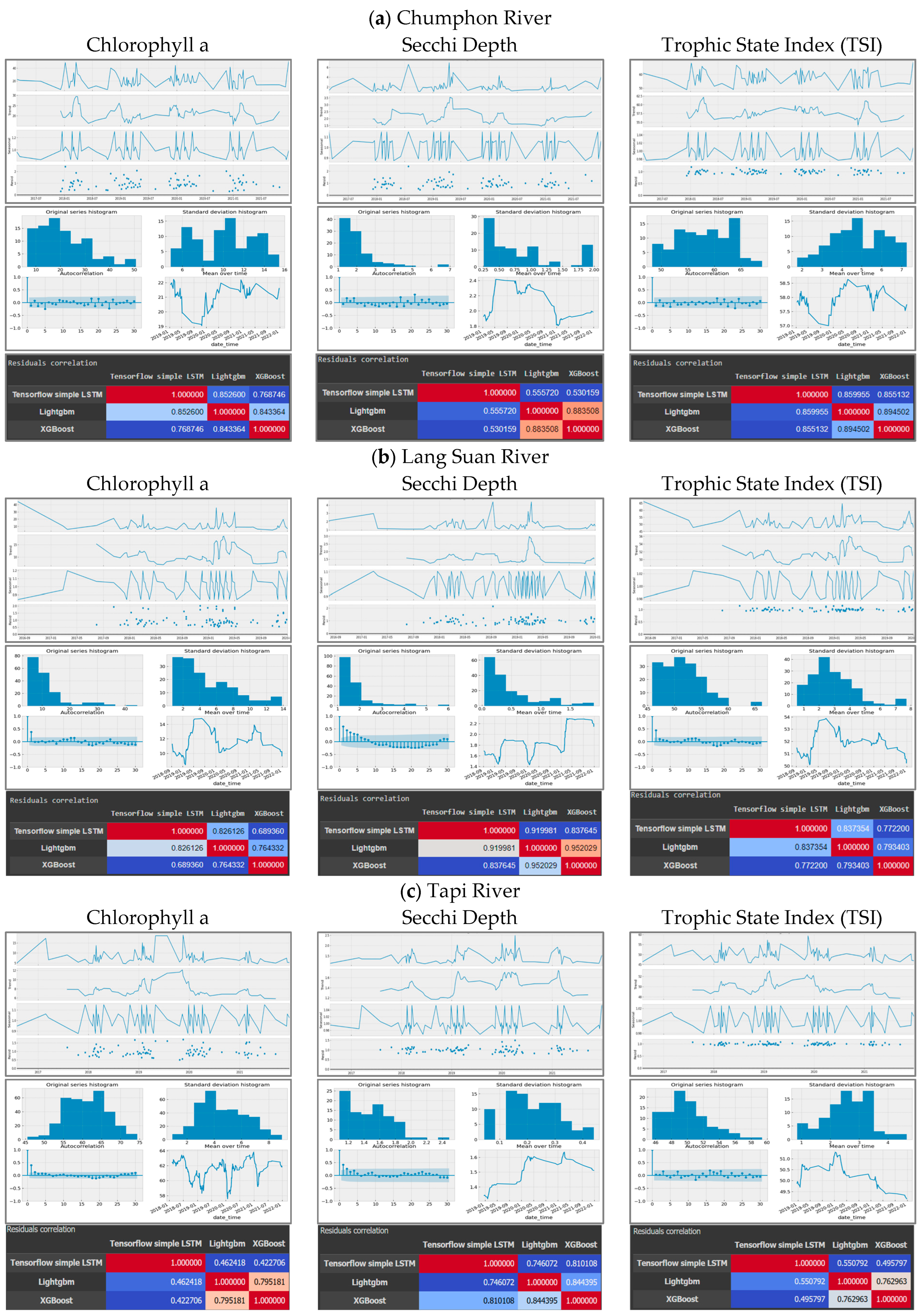
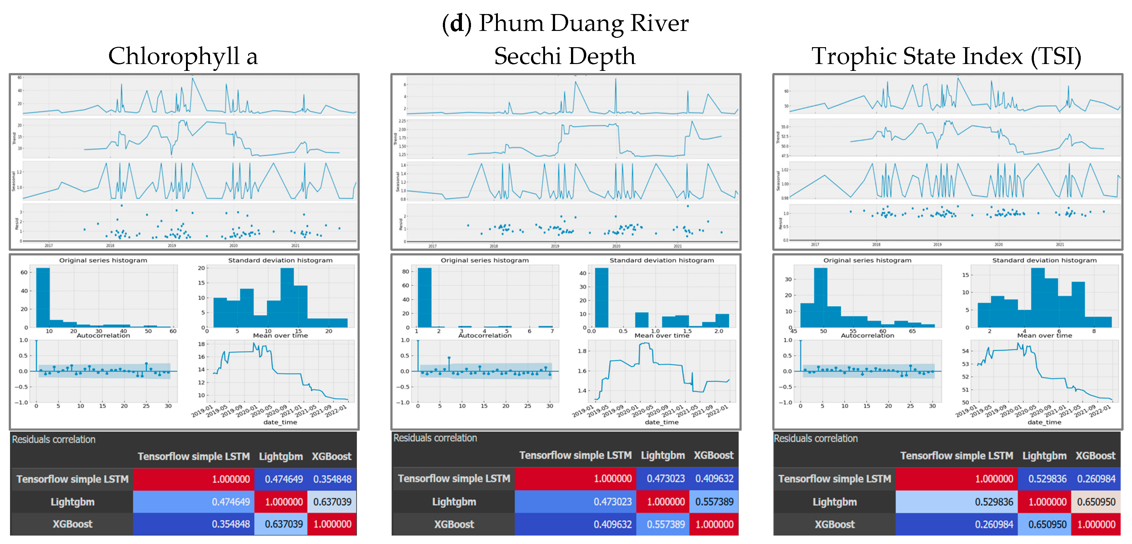
3.3.3. Model Comparison Framework

To test Hypotheses H1 and H2, we conducted a comparative analysis of multiple forecasting models for each water quality parameter. Chlorophyll-a, known for its nonlinear patterns and abrupt fluctuations due to algal bloom events, was modelled using nonlinear machine learning approaches such as Support Vector Machines (SVM) with RBF kernel. In contrast, parameters exhibiting seasonal and linear trends—such as Secchi Depth and the Trophic State Index—were modelled using traditional time series models, particularly ARIMA and SARIMAX.

Each model’s forecasting accuracy was evaluated using standard statistical metrics: Mean Absolute Error (MAE), Root Mean Square Error (RMSE), and Mean Absolute Scaled Error (MASE). The comparative model analysis was performed for each monitoring station to assess spatiotemporal generalizability and robustness.

While grid search was employed for SVM-RBF parameter tuning (C: 0.1–100; γ: 0.001–1), we acknowledge that metaheuristic approaches (e.g., Bayesian optimisation, genetic algorithms) may offer efficiency advantages in complex parameter landscapes [44,45]. The grid search approach was selected to ensure reproducible benchmarking across all stations, with the full parameter space explored given available computational resources. Future implementations could benefit from adaptive optimisation methods when scaling to larger regions or higher-frequency forecasting.

4. Results

4.1. Estimation and Spatial Distribution of Water Quality Parameters

This section evaluates water quality parameters estimated using Sentinel-2 imagery processed via Google Earth Engine. Empirical algorithms were applied to derive Chlorophyll-a, Secchi Depth, and the Trophic State Index (TSI)—three indicators reflecting algal biomass, water transparency, and productivity, respectively. Spectral indices derived from optimal Sentinel-2 bands were statistically summarised (

Table 5. Summary statistics of Sentinel-2-derived water quality parameters (2017–2022).

Parameter	Unit	Mean	Standard Deviation (SD)	Median	Maximum	Minimum
Chlorophyll a	mg/L	19.685	15.956	13.540	99.871	4.503
Secchi Depth	m	2.004	1.109	1.593	9.855	1.081
Trophic State Index (TSI)	–	56.178	6.257	54.930	75.764	45.361

), revealing mean Chlorophyll-a at 19.69 mg/L, moderate water transparency (~2.00 m), and a mesotrophic-average TSI of 56.18. These parameters reflect significant variability and provide ecological insights into the monitored rivers.

Spatial patterns of these parameters are visualised in Figure 2, illustrating distribution across four river systems. Notably, Lang Suan and Tapi Rivers show elevated Chlorophyll-a near estuarine zones, while Phum Duang consistently displays greater transparency.

4.2. Temporal Variability of Water Quality Parameters

Using Sentinel-2-derived time series data from 2017 to 2022, we analysed seasonal and inter-annual dynamics of water quality indicators (Figure 3).

• Seasonal Trends: Chlorophyll-a peaks post-monsoon (Oct–Dec), particularly near estuaries (e.g., LS01, TP01), suggesting nutrient inflow effects. Secchi Depth declines during the monsoon (May–Sep) due to turbidity. TSI tracks Chlorophyll-a, peaking in dry seasons.
• Inter-Annual Variation: Upstream stations (e.g., TP07) maintain greater consistency in clarity. Chumphon River experiences the highest TSI fluctuation, likely from tidal and urban influence.

4.3. Results of Time Series Forecasting of Water Quality Parameters

This section evaluates the performance of models in forecasting water quality indicators using machine learning (SVM, LSTM) and statistical (ARIMA, SARIMAX) methods. Forecasts were validated across multiple stations using standard metrics such as MAE, RMSE, MAPE, and wQL.

4.3.1. Overall Performance of Amazon Forecast

Table 6. Performance of Amazon forecast models across parameters.

Parameter	MASE	RMSE	MAPE	Average wQL	wQL (0.1)	wQL (0.5)	wQL (0.9)
Chlorophyll a	0.8662	28.7088	0.4410	0.4013	0.2254	0.6533	0.3253
Secchi Depth	0.7394	3.1251	0.3350	0.3952	0.1939	0.6796	0.3210
Trophic State	0.8397	63.8243	0.2635	0.3264	0.2271	0.5379	0.2142

summarises the performance of Amazon Forecast across the three parameters. Results show the following:

• Chlorophyll-a exhibited the highest RMSE (28.71) and MAPE (44.10%), indicating forecasting challenges likely due to high spatiotemporal variability and nonlinearity.
• Secchi Depth was modelled more effectively, with a lower MASE (0.7394) and MAPE (33.5%), consistent with its smoother seasonal patterns.
• The Trophic State Index achieved the lowest MAPE (26.35%), showing stable predictions in moderately fluctuating systems.

Notably, wQL values rise at higher quantiles, especially for Chlorophyll-a, suggesting greater difficulty in predicting extreme events (e.g., algal blooms).

4.3.2. Station-Level Model Comparisons

Table 7. Comparative performance of forecasting models across monitoring stations.

Station	Parameter	Models	MAE	RMSE	MASE
CP01	Chlorphyll-a	Randomforest	0.79	10	0.5
		ARIMA	0.8	10	0.52
		Naive mean	0.81	10	0.54
	Secchi Depth	Lasso	0.48	0.7	0.23
		BayesianRidge	0.49	0.8	0.24
		Lightgbm	0.49	0.8	0.25
	Trophic	ARIMA	5.2	6.2	0.09
		SVM RBF GRID SEARCH	5.3	6.3	0.09
		BayesianRidge	5.3	6.2	0.09
		BayesianRidge	5.3	6.2	0.091
LS01	Chlorphyll-a	SARIMAX	3.2	5.8	0.3
		ARIMA	3.4	5	0.37
		AR	3.4	5.1	0.37
	Secchi Depth	SARIMAX	0.41	0.76	0.21
		ARIMA	0.43	0.77	0.23
		AutoSARMAX(1,0,1),(0,0,0,6)	0.44	0.78	0.25
	Trophic	SARIMAX	2.3	3.5	0.03
		AR	2.4	3.6	0.04
		ARIMA	2.4	3.7	0.04
TP01	Chlorphyll-a	SVM RBF GRID SEARCH	1.3	1.8	0.2
		ARIMA	1.7	2	0.28
		SARIMAX	1.9	2.2	0.24
	Secchi Depth	Randomforest	0.21	0.28	0.13
		EnsembleXG + LIGHT	0.22	0.29	0.15
		BayesianRidge	0.23	0.28	0.15
	Trophic	SVM RBF GRID SEARCH	3.2	3.3	0.03
		ARIMA	3.2	3.3	0.04
		Naive mean	3.3	3.4	0.06
TP04	Chlorphyll-a	SVM RBF GRID SEARCH	5.6	8.3	0.6
		SARIMAX	6.2	9.8	0.5
		ARIMA	8.1	9.2	0.9
	Secchi Depth	SVM RBF GRID SEARCH	0.3	0.7	0.2
		ARIMA	0.4	0.8	0.3
		Naive mean	0.5	0.9	0.35
	Trophic	Tensorflow simple LSMT	3.8	4.3	0.13
		SARIMAX	3.9	5	0.12
		EnsembleXG + TF	3.9	4.3	0.14

compares multiple models (e.g., SVM, Random Forest, ARIMA, SARIMAX, LSTM) across key monitoring stations. Performance varied by parameter and location as follows:

• SVM RBF GRID SEARCH consistently outperformed other models for Chlorophyll-a at TP01 and TP04, supporting Hypothesis H1 regarding nonlinear data.
• For Secchi Depth, Lasso, Bayesian Ridge, and Random Forest models achieved MAE < 0.5 across most sites, validating the use of more straightforward or linear models for this parameter (Hypothesis H2).
• TSI forecasting showed similar performance for ARIMA, SVM, and TensorFlow-based models, suggesting hybrid models (e.g., EnsembleXG + TF) may be more adaptive to regional heterogeneity.

In addition to the standard RBF kernel, we evaluated a hybrid polynomial–RBF kernel at select stations (TP04 and LS01) to assess its ability to capture mixed signal patterns. While the hybrid kernel achieved a slight RMSE reduction (2.7–3.1%) over the pure RBF, this came at the cost of increased model complexity and longer training times (≈42% higher). These results suggest that hybrid kernels may offer marginal gains in heterogeneous environments, but the added computational burden may limit their practical applicability for real-time systems.

4.4. Estimation of Additional Water Quality Parameters Using Regression Models

This section presents the simulation results of water quality parameter estimation using regression-based machine learning models trained on Sentinel-2 satellite imagery. The analysis focused on three critical water quality indicators—Dissolved Oxygen (DO), Biochemical Oxygen Demand (BOD), and Faecal Coliform Bacteria (FCB)—due to their relevance for aquatic ecosystem health and pollution detection.

To ensure temporal alignment and data integrity, only remotely sensed values corresponding to actual in situ monitoring dates were selected for training and evaluation. The goal was to assess how accurately these parameters could be estimated from spectral features derived from satellite data.

4.4.1. Descriptive Statistics

Table 8. Summary of observed in situ water quality parameters used for regression modelling.

Parameter	Unit	Mean	SD	Median	Max	Min
DO	mg/L	6.260	1.089	6.396	8.748	1.089
BOD	mg/L	2.324	21.852	1.437	570.814	0.540
FCB	MPN/100 mL	3674.96	12,371.40	1574.60	162,797.07	−12,264.81

summarises the distribution of observed values used in the regression modelling. The data distribution highlights distinct levels of variability. DO exhibited a relatively narrow range, consistent with its biochemical stability under natural conditions. Conversely, BOD and FCB displayed extreme variability, with BOD reaching anomalously high values and FCB containing negative outliers, suggesting potential data entry or processing issues that require cleaning or transformation before modelling.

4.4.2. Regression Model Performance

The predictive performance of the regression models is reported in

Table 9. Performance metrics of regression models for estimating water quality parameters.

Parameter	MAE	MSE	RMSE	R²	RMSLE	MAPE
DO	0.8898	1.4709	1.1961	0.3762	0.2080	0.3434
BOD	0.5655	0.6190	0.7668	0.0965	0.2816	0.5240
FCB	3212.47	208,466,710	9885.99	0.2717	1.7880	24.9301

, based on six evaluation metrics: MAE, MSE, RMSE, R², RMSLE, and MAPE. These metrics were chosen to capture absolute accuracy and sensitivity to variance and skewed distributions.

The model for Dissolved Oxygen yielded the strongest performance, with an R² of 0.3762 and a relatively low RMSE (1.1961), indicating moderate predictive capability using remote sensing features. Despite a lower error in terms of MAE and RMSE, BOD achieved an R² of only 0.0965, suggesting that the model captured limited variance in the ground truth values. The regression model for FCB, a microbial parameter influenced by numerous stochastic and anthropogenic factors, exhibited the highest prediction error and lowest robustness, with RMSE exceeding 9800 and MAPE approaching 25%.

4.4.3. Interpretation and Model Implications

These findings confirm that physicochemical parameters, such as dissolved oxygen (DO), which are directly or indirectly linked to optical properties detectable by satellites, can be estimated with reasonable accuracy. Meanwhile, parameters with episodic, nonlinear behaviours—such as FCB and BOD—remain challenging to model from spectral data alone due to the influence of local, non-visible drivers (e.g., sewage discharges, rainfall events, microbial growth dynamics).

The results highlight the potential of integrating satellite data and regression-based machine learning for near-real-time monitoring of select water quality parameters. However, they also emphasise the importance of:

• Incorporating additional environmental or hydrological covariates (e.g., precipitation, land use),
• Handling outliers and skewed distributions through robust preprocessing,
• Applying log or power transformations where appropriate.

5. Discussion

This study presents a comprehensive and data-rich approach for assessing and forecasting surface water quality in tropical river systems by integrating Sentinel-2 remote sensing data with machine learning and time series models. The work advances the field in four major ways: (1) it enhances temporal and spatial monitoring coverage, (2) it applies model-specific forecasting aligned to the nature of each water quality parameter, (3) it develops a visual interface for stakeholder engagement, and (4) it establishes a replicable framework for data-scarce estuarine environments.

5.1. Interpretation of Findings and Parameter-Specific Model Suitability

The results demonstrated significant variation in the forecastability and spatial coherence of different water quality parameters:

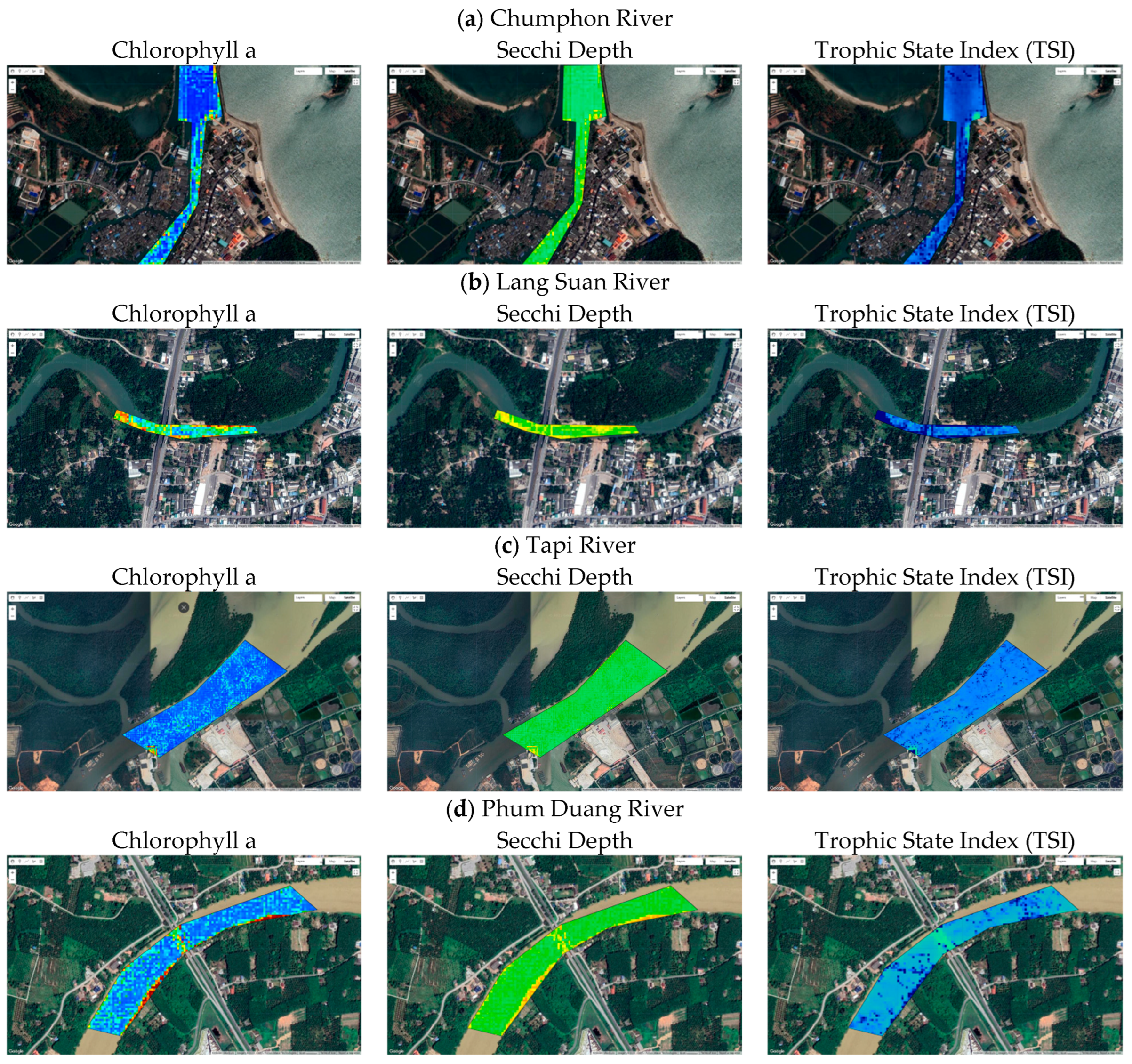
5.1.1. Chlorophyll-a

This parameter, indicative of phytoplankton biomass and potential eutrophication, was the most challenging to forecast, primarily due to nonlinear, high-frequency fluctuations caused by nutrient loading, weather, and tidal influences. Despite these complexities, SVM with RBF kernel consistently outperformed linear methods such as ARIMA. This is likely due to the ability of nonlinear kernels to capture chaotic relationships in phytoplankton dynamics—confirming our Hypothesis H1 and aligning with similar results in coastal studies from India and the South China Sea. The performance of SVM-RBF reinforces its role as a viable operational model in eutrophic and anthropogenically influenced systems, where bloom prediction is crucial for public health and fisheries management.

5.1.2. Secchi Depth

This parameter exhibited strong seasonality and linear trends, influenced mostly by sediment load, turbidity, and flow conditions. As expected, ARIMA, Bayesian Ridge, and Lasso regression offered high accuracy with low RMSE and MAE values, supporting Hypothesis H2. These findings are consistent with those of Laosuwan et al. (2022) [16], who also reported stable forecast accuracy for transparency indices in Thailand’s upper Gulf using the ARIMA model. Simpler, computationally efficient linear models can often be preferred in resource-constrained monitoring systems for parameters such as transparency, as they require less hyperparameter tuning and training time.

5.1.3. Trophic State Index (TSI)

TSI, which combines information from Chlorophyll-a and Secchi Depth, exhibited moderate fluctuations. It demonstrated good predictability across multiple models, but the TensorFlow-based LSTM model performed best in ecologically heterogeneous systems, such as TP04, partially validating Hypothesis H2 and emphasising the value of deep learning in dynamic, mixed-signal environments. The hybrid nature of TSI—comprising both nonlinear and seasonal components—makes it ideal for ensemble or hybrid forecasting strategies, which combine ARIMA, SVM, and neural networks.

5.2. Regression Modelling of Biochemical Parameters: Challenges and Potentials

The regression models showed mixed performance when estimating non-optically active parameters:

• Dissolved Oxygen (DO): Predictive accuracy was moderate (R² ≈ 0.38), indicating partial spectral visibility, likely through correlation with algal activity and water clarity.
• Biochemical Oxygen Demand (BOD) and Faecal Coliform Bacteria (FCB): These were poorly estimated, with high RMSE and low R² scores, primarily due to their stochastic behaviour and indirect relationship with optical properties.

Remote sensing-based modelling of microbiological or chemical parameters is feasible only when ground-based explanatory variables (e.g., rainfall, land use, sewerage infrastructure) are integrated. Future work should prioritise data fusion approaches that combine satellite, meteorological, and anthropogenic data sources to better capture causality and enhance model generalisation.

5.3. Benchmarking Against Existing Literature

This study demonstrates significantly improved predictive performance, particularly for Chlorophyll-a and dissolved oxygen (DO), compared to previous modelling efforts (

Table 10. Comparison of modelling approaches for coastal water quality forecasting in tropical regions.

Study	Region	Modelling Approach	Parameters Forecasted	RMSE/Accuracy	Data Source
[16]	Upper Gulf of Thailand	ARIMA, linear regression	Chlorophyll-a, TSS	RMSE: 6.2 (Chl-a)	Landsat 8 + field data
[22]	India (Goa estuary)	Random Forest	BOD, DO, FCB	R² = 0.45 (DO)	Sentinel-2 + field data
[66]	South China Sea	LSTM, Bi-LSTM	Chlorophyll-a	RMSE: 3.4	MODIS + remote sensing indices
[34]	Global tropical estuaries	ANN, PCA regression	Turbidity, TSI	RMSE: 5.8–9.2	Landsat/MODIS
This study (2025)	Gulf of Thailand	SVM-RBF, ARIMA, LSTM, XGBoost	Chlorophyll-a, DO, Secchi, TSI, FCB	RMSE: 1.8 (Chl-a), 1.2 (DO), 3.1 (Secchi), 4.3 (TSI)	Sentinel-2 + 3777 entries + ground truth

) in the Gulf of Thailand and similar tropical estuarine environments. For instance, Laosuwan et al. (2022) [16] applied traditional ARIMA and regression models in the upper Gulf, reporting an RMSE of 6.2 for Chlorophyll-a, while our hybrid approach using SVM-RBF reduced this error to 1.8. Similarly, Jin et al. (2021) [66] utilised LSTM networks in the South China Sea, achieving RMSE values above 3.0 for Chlorophyll-a. Our tailored application of ensemble models and nonlinear learning yielded better accuracy with additional spatial refinement. In contrast to earlier studies that relied solely on MODIS or Landsat imagery with limited temporal granularity, our use of Sentinel-2 imagery combined with over 3700 matched ground truth observations significantly enhanced both spatial and temporal resolution. These improvements affirm the added value of multi-model, multi-source data fusion in dynamic and anthropogenically influenced coastal zones such as the Gulf of Thailand. This study demonstrates that high-resolution remote sensing, when paired with appropriate machine learning models, can significantly enhance forecasting accuracy and data continuity even in data-scarce settings.

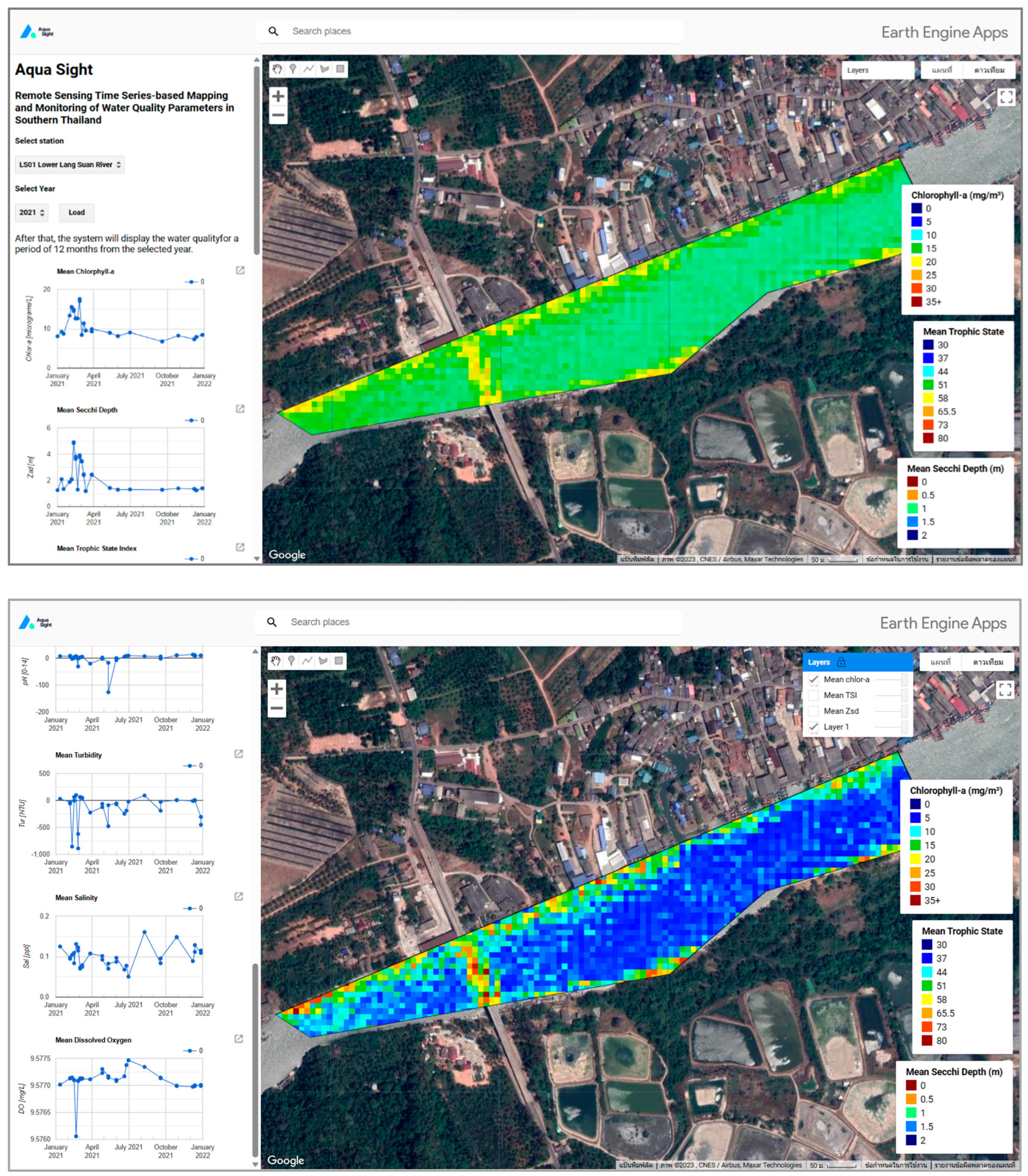
5.4. Platform Deployment and Decision-Making Support

The deployment of Aqua Sight (Figure 4), a web-based visualisation platform built with Google Earth Engine and Streamlit, demonstrates the practical applicability of this research. The tool supports multi-parameter time series visualisation, aiding environmental agencies in real-time assessment and early warning of potential ecological risks. This user-oriented design aligns with the growing need for operational monitoring tools in rapidly developing coastal regions. Aqua Sight represents a scalable model for digital environmental governance, supporting real-time interventions in water management, particularly in contexts where regulatory compliance and public awareness are limited.

5.5. Hypotheses Revisited

The findings of this study align well with the hypotheses proposed at the outset:

I.

H1 was supported. Chlorophyll-a, which exhibits nonlinear and spatiotemporally erratic behaviour due to algal blooms, was most accurately predicted using SVM with RBF kernel. This confirmed that nonlinear models better handle the complexity of this parameter, as evidenced by lower RMSE values compared to ARIMA and naive baselines.

II.

H2 was partially supported. ARIMA consistently outperformed more complex machine learning models for Secchi Depth, which follows relatively stable seasonal cycles. However, for TSI, results varied across stations. While ARIMA performed well in many cases, hybrid and deep learning models (e.g., EnsembleXG + TF) offered competitive or better performance in heterogeneous systems, suggesting that a mixed-model strategy may be more suitable.

III.

H3 was confirmed. Integrating remote sensing-derived indices with machine learning enabled the generation of high-frequency, spatially resolved water quality forecasts, achieving data coverage 5.4 times greater than traditional monitoring. This validates the hypothesis that fusing satellite data with advanced modelling techniques enhances spatial granularity and forecasting robustness.

These outcomes underscore the value of hypothesis-driven modelling in environmental informatics and contribute to the growing body of evidence supporting AI-augmented monitoring systems for complex aquatic ecosystems.

5.6. Limitations and Recommendations

While the integrated approach significantly expands data availability and improves forecasting capabilities, some limitations must be acknowledged:

• Data sparsity and noise in ground-truth measurements impacted model accuracy, especially for microbiological parameters.
• Temporal mismatches between satellite overpasses and field sampling may introduce errors in model calibration.
• Future research should explore data fusion approaches (e.g., combining satellite with rainfall, flow, or land use data) and deep learning architectures (e.g., attention-based temporal networks) for enhanced generalisation.

Furthermore, future studies may benefit from testing recent deep learning architectures, such as TabNet, which combines attentive feature selection with interpretability specifically for tabular data. Its potential for capturing complex feature interactions while providing model transparency makes it a promising alternative to traditional tree-based and kernel-based methods. Comparative benchmarking against TabNet and similar frameworks could yield further insights into optimising accuracy and explainability for remote sensing-derived water quality predictions.

6. Conclusions

This study presents an integrated framework that combines Sentinel-2 remote sensing with machine learning and time series models to monitor and forecast surface water quality in the Gulf of Thailand. The system effectively captured both spatial variability and temporal trends for key indicators, including Chlorophyll-a, Secchi Depth, Trophic State Index, and select physicochemical parameters (DO, BOD, FCB).

Results showed that nonlinear models (e.g., SVM with RBF kernel, LSTM) outperformed traditional approaches for dynamic parameters, such as Chlorophyll-a, while autoregressive models were more effective for seasonally stable indicators, such as Secchi Depth. These findings highlight the importance of parameter-specific model selection.

By reducing dependence on manual sampling, the framework significantly improves monitoring coverage and forecasting accuracy. The accompanying Aqua Sight platform demonstrated its real-time application potential, supporting informed decision making for environmental agencies.

This approach offers a scalable, cost-efficient solution for sustainable water quality management in data-limited and ecologically complex regions. To enhance future performance, integrating multi-source environmental data (e.g., rainfall, land use, nutrient inputs) and adopting explainable AI techniques will be essential. Continued model updates and long-term forecasting will ensure adaptability to evolving environmental and climate conditions.