Article

Patterns, Risks, and Forecasting of Irrigation Water Quality Under Drought Conditions in Mediterranean Regions

1
Instituto Politécnico de Beja, Escola Superior Agrária de Beja, Campus do Instituto Politécnico de Beja, 7800-295 Beja, Portugal
2
Center for Sci-Tech Research in Earth System and Energy (CREATE), Instituto Politécnico de Beja, Campus do Instituto Politécnico de Beja, 7800-295 Beja, Portugal
3
GeoBioTec, Nova School of Science and Technology, Campus da Caparica, 2829-516 Caparica, Portugal
4
Department of Computer Science, Nova School of Science and Technology, Campus da Caparica, 2829-516 Caparica, Portugal
5
Centro Operativo e de Tecnologia de Regadio, Quinta da Saúde, Apartado 354, 7800-999 Beja, Portugal
6
Águas Publicas do Alentejo, Grupo Águas de Portugal, Rua Dr. Aresta Branco nº 51, 7800-310 Beja, Portugal
*
Author to whom correspondence should be addressed.
Water 2025, 17(12), 1783; https://doi.org/10.3390/w17121783
Submission received: 13 May 2025 / Revised: 4 June 2025 / Accepted: 12 June 2025 / Published: 14 June 2025

Abstract

The seasonal and interannual irregularity of temperature and precipitation is a feature of the Mediterranean climate that is intensified by climate change and constitutes a relevant driver of water and soil degradation. This study was developed during three years in a hydro-agricultural area of the Alqueva irrigation system (Portugal) with Mediterranean climate conditions. The sampling campaigns included collecting water samples from eight irrigation hydrants, analyzed four times yearly. The analysis incorporated meteorological data and indices (precipitation, temperature, and drought conditions) alongside chemical parameters, using multivariate statistics (factor analysis and cluster analysis) to identify key water quality drivers. Additionally, machine learning models (Random Forest regression and Gradient Boosting machine) were employed to predict electrical conductivity (ECw), sodium adsorption ratio (SAR), and pH based on chemical and climatic variables. Water quality evaluation showed a prevalence of a slight to moderate soil sodification risk. The factor analysis outcome was a three-factor model related to salinity, sodicity, and climate. The cluster analysis revealed a grouping pattern led by year and followed by stage, pointing to the influence of inter-annual climate irregularity. Variations in water quality from the reservoirs to the distribution network were not substantial. The Random Forest algorithm showed superior predictive accuracy, particularly for ECw and SAR, confirming its potential for the reliable forecasting of irrigation water quality. This research emphasizes the importance of integrating time-sensitive monitoring with data-driven predictions of water quality to support sustainable water resources management in agriculture. This integrated approach offers a promising framework for early warning and informed decision-making in the context of increasing drought vulnerability across Mediterranean agro-environments.

1. Introduction

Droughts are becoming more common in Mediterranean regions, with increasingly unpredictable rainfall patterns [1,2]. This variability, heightened by global climate change, poses a serious threat to food security. Traditional farming schedules are disrupted and water scarcity during key crop-growing periods threatens crop yields [1,2].
Besides the impacts of droughts on water quantity, the quality of water for agricultural and other uses is also compromised [3,4]. The effects of erratic precipitation distribution and interannual climate variability on the deterioration of surface and groundwater quality have been widely reported and are expected to worsen with global climate change [5,6,7,8,9,10,11]. Extreme precipitation events can increase runoff, which subsequently causes soil erosion but also transports organic pollutants like pesticides into water bodies, thus resulting in a degradation of water quality [12,13]. Higher temperatures contribute to rising evaporative rates, concentrating dissolved salts and nutrients in water bodies [14]. Extended periods of drought reduce water flows, causing the concentration of contaminants and decreasing the dilution of pollutants [15,16].
The expansion of irrigation systems in drought-prone areas has raised concerns about soil degradation, particularly salinization and the overall loss of soil health [17,18]. In fact, soil salinization is one of the critical physical–chemical degradation processes in drought-prone regions where irrigation is adopted [19,20]. Salt-affected soils occupy more than 20% of the global irrigated area and, in some countries, they occur in more than half of the irrigated land [21]. In the Mediterranean region, 25% of the irrigated cropland is affected by moderate-to-high salinization [22].
Hillel (2000) and Hillel et al. (2008) [19,23] highlighted the importance of having early warning systems to detect salinity and sodicity in irrigated agroecosystems. Besides the routine water monitoring programs in surface or groundwater bodies that supply irrigation perimeters, the diversification of spatial and temporal monitoring could predict the onset of salinization processes, especially when usual patterns of humid and dry periods are disturbed by drought occurrence [24]. Recently, data-driven approaches such as machine learning (ML) have emerged as tools to support environmental monitoring and forecasting. Several studies have highlighted the use of ML to predict water quality based on algorithms like Artificial Neural Networks, Random Forest, Multiple Linear Regression, Gradient Boosting, Support Vector Machines, or K-Nearest Neighbors, among others [25,26,27,28]. A prediction of stream water quality based on both chemical and meteorological data was performed by [29] using the RF and Boosted regression tree (BRT) models. Some recent studies have specifically focused on modeling irrigation water quality, typically relying on datasets of physicochemical parameters to predict indices or key target variables [30,31,32]. Machine learning algorithms can handle complex, nonlinear relationships between large sets of variables, allowing for the prediction of key salinity indicators, the identification of the most influential parameters contributing to water degradation in irrigated systems, and the modernization of irrigation water quality management [33]. While these studies have explored the use of predictive models for irrigation water quality, to the best of our knowledge, none have integrated meteorological variables that describe cumulative dryness during drier years. In this context, the use of ML in irrigation water quality monitoring under climate uncertainty can enhance early detection of salinization risks and support more adaptive water management strategies.
This study aims to evaluate irrigation water quality at the hydrant level under drought conditions and to explore the potential of ML models in predicting key irrigation water quality parameters. Specifically, the objectives are (i) to evaluate the suitability of irrigation water for agricultural use during dry periods, (ii) to evaluate the contribution of hydrant-level water quality assessment to improve spatial monitoring, (iii) to identify the most influential factors affecting water quality variability under drought conditions, and (iv) to compare the performance of two ML algorithms, Random Forest and Gradient Boosting, in predicting salinity-related parameters from chemical and meteorological variables.

2. Materials and Methods

2.1. Study Area

This study was conducted in eight hydrants (H5, H6, H7, H16, H21, H22, H23, and H33, as identified by the water supplier company) distributing water to ten farm fields with a land use of drip-irrigated vineyards and olive orchards and sprinkler-irrigated annual field crops, forages, and pastures (Table 1), totaling 88 ha. All farm fields were located in the Brinches-Enxoé hydro-agricultural area with an equipped area of 5061 ha, part of the Alqueva irrigation system, in the Alentejo region, South Portugal (Figure 1). The conveyance networks of the Brinches-Enxoé hydro-agricultural area originate in the Laje (pressurized) and the Montinhos (gravity) reservoirs, respectively. The former is the upstream reservoir of all the studied hydrants, except for H16, supplied by Montinhos.
The predominant soil types are medium to fine-textured calcaric cambisols, chromic vertisols, and chromic luvisols [34], represented in Figure 1.
The climate in the region is temperate with a hot and dry summer (Mediterranean) with an annual precipitation and average mean monthly temperature of, respectively, 558 mm and 16.9 °C (1981–2010 climatological normal; [35]).

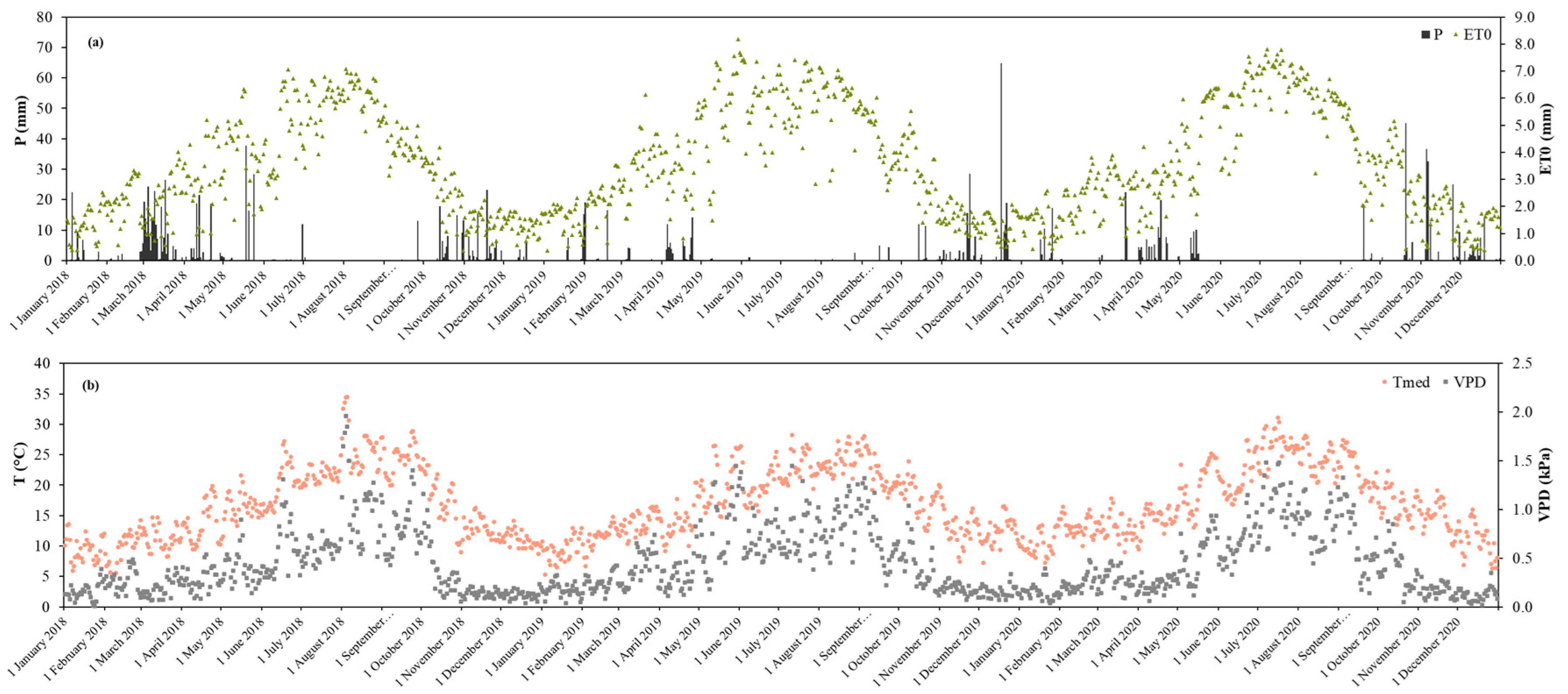
2.2. Meteorological Data and Drought Characterization

Meteorological data were recorded in an automatic meteorological station of the Irrigation Operating and Technology Center (Centro Operativo e de Tecnologia do Regadio—COTR) located in the area (37.97 N; 7.55 W) [36]. To characterize the meteorological trends during the study period, the monthly Standard Precipitation Index (SPI) was calculated [37]. The SPI is a statistical index that measures precipitation anomalies in a given region and time compared to historical patterns. It was obtained by fitting the long-term monthly precipitation records of the period 1981–2010 [38] to a Gamma probability distribution, which was then transformed into a normal distribution. Droughts can be classified as mild, for −1.0 < SPI < 0; moderate, if −1.5 < SPI ≤ −1.0; severe, for −2.0 < SPI ≤ −1.5; and extreme, if SPI ≤ −2.0.
The occurrence of drought was identified according to [37] as a period in which the SPI is continuously negative and reaches a value ≤ −1.0, beginning when the SPI first falls below zero and ending with a positive value of the SPI following a value ≤ −1.0. The duration (number of months), magnitude (∑|SPI| during drought), and intensity (magnitude/duration) of droughts were also evaluated.
The values of accumulated precipitation (Pcum) and accumulated reference evapotranspiration (ET0cum) until each sampling date were computed to obtain variables in the dataset that could be descriptive of the meteorological conditions when applying the multivariate statistical methods and the ML model.

2.3. Sampling Strategy

This study covered 12 water sampling campaigns, with four campaigns each year, performed in April–May, June–July, September–October, and November, corresponding to the following assigned stages of crop development/irrigation season, respectively: Initial (I); Middle (M); Late (L); and Post-cycle (P). For the assessment, 2 L water samples were collected in polyethylene bottles from the irrigation hydrants. The samples were transported to the laboratory in a cooler at 4 °C and stored, following the requisites for water conservation for each parameter [39].
Water pH was determined by potentiometry with a pH probe, and ECW was determined by conductometry with a conductivity meter. The concentrations of ions of calcium (Ca), magnesium (Mg), sodium (Na), chloride (Cl), boron (B), and nitrate (NO3) were determined by the ionic chromatography methodology [39].

2.4. Irrigation Water Quality Assessment

The assessment of water quality for irrigation was performed using the consensual guidelines of the Food and Agriculture Organization of the United Nations (FAO) (Table S1), which consider four types of “potential problems” that can arise from the use of poor quality irrigation water, namely (i) salinity, which can affect soil water availability; (ii) infiltration rate of water into the soil; (iii) specific ion toxicity in sensitive crops; (iv) and miscellaneous effects on susceptible crops [40].

2.5. Exploratory Statistical Analyses

Matrices of Spearman’s correlation coefficients were computed for preliminary examination of the relationships between variables. Factor and cluster analyses were performed to explore data structure and case similarity using the methodology described in Tomaz et al. [41,42]. Analyses were performed with Statistica 7 [43].

2.6. Machine Learning Models

Random Forest (RF) and Gradient Boosting (GB) models were tested to forecast three key indicators of irrigation water quality (target variables), ECW, SAR, and pH, using a dataset of the average values of continuous physicochemical and meteorological predictors: Pcum, ET0cum, B, Ca, Mg, Na, Cl, and NO3.
RF is a supervised ensemble ML model based on a collection of decision trees (estimators) [44]. Because it is an ensemble technique, it uses the best outcome given by the many decision trees, mitigating and limiting generalization mistakes as the volume of the tree architecture in the forest grows. In addition, it shows the ability to capture nonlinear relationships [28,30].
GB is also a supervised ensemble ML model that uses decision trees as base learners, but builds them sequentially, with each new tree focusing on correcting the prediction errors made by the previous ones. This boosting approach enables the model to gradually improve its accuracy by minimizing a loss function at each step [45].
Both models were developed in Visual Studio Code(version 1.100.1 Python 3.10) using Python libraries, such as scikit-learn, pandas, and matplotlib. For each target variable, the RF models were trained with 100 decision trees, which is the default configuration recommended in the library as a balance between predictive performance and computational efficiency. Similarly, the GB models were also trained using the default hyperparameters, including 100 decision trees and a learning rate of 0.1, which controls how much each new tree influences the final model. Model evaluation was performed using an 80–20% train–test split of the dataset, meaning that the RF algorithm built an input–output relationship with 80% of the dataset and subsequently generalized or predicted outputs for the 20% of unseen inputs [28,46]. For each algorithm and model, the following performance metrics were calculated: coefficient of determination (R2), root mean square error (RMSE), mean absolute error (MAE), and relative bias (RBIAS). The final model was selected based on cross-validated performance metrics (R2, RMSE, MAE, etc.). In addition, the mean decrease in impurity (MDI), or Gini importance, was used to rank the feature importance (of each predictor) in the RF model [47]. Measured and predicted values of each parameter were represented in scatter plots to evaluate the accuracy and goodness of fit for both models.

3. Results and Discussion

3.1. Meteorological Trends and Drought Characterization

The annual precipitation was 603 mm, 343 mm, and 615 mm in 2018, 2019, and 2020, respectively, while the mean annual temperature was 16.7 °C, 17.3 °C, and 17.8 °C. The mean temperature during the growing/irrigation season of the different crops in the study area (March to October) each year was 19.8 °C, 20.2 °C, and 20.5 °C, respectively. The year 2018 was characterized by high precipitation in the spring (March and April) and autumn (October and November); 2019 was a very dry year, characterized by high temperatures and very low precipitation; 2020 registered higher mean monthly temperatures, and despite presenting higher annual precipitation than the two previous years, rain was mostly concentrated in April and the autumn months (October and November) (Figure 2).
Calculations of the monthly SPI were made to better understand the climate’s interannual and seasonal variability during the period of the study and the occurrence of drought (Figure 2).
A continuing trend of dry conditions started from the end of 2018 through the end of 2019 and the initial months of 2020, with the occurrence of four almost consecutive droughts (Figure 3). The longest drought lasted 5 months (1 December 2018 to 1 April 2019), but the highest drought magnitude occurred from 1 May 2019 to 1 August 2019, when the minimum SPI reached −2.73, signaling extreme dry weather. These dry conditions continued until the end of 2019 (November). The drought persisted until 1 March 2020. During 2019, precipitation values were consistently lower than the climatological normal (except in April and December), which, along with the high temperatures, contributed to the year’s severe dry conditions. In 2020, there was a recovery in precipitation levels, especially in March–April and October–November, but temperatures remained higher than historical records [48].

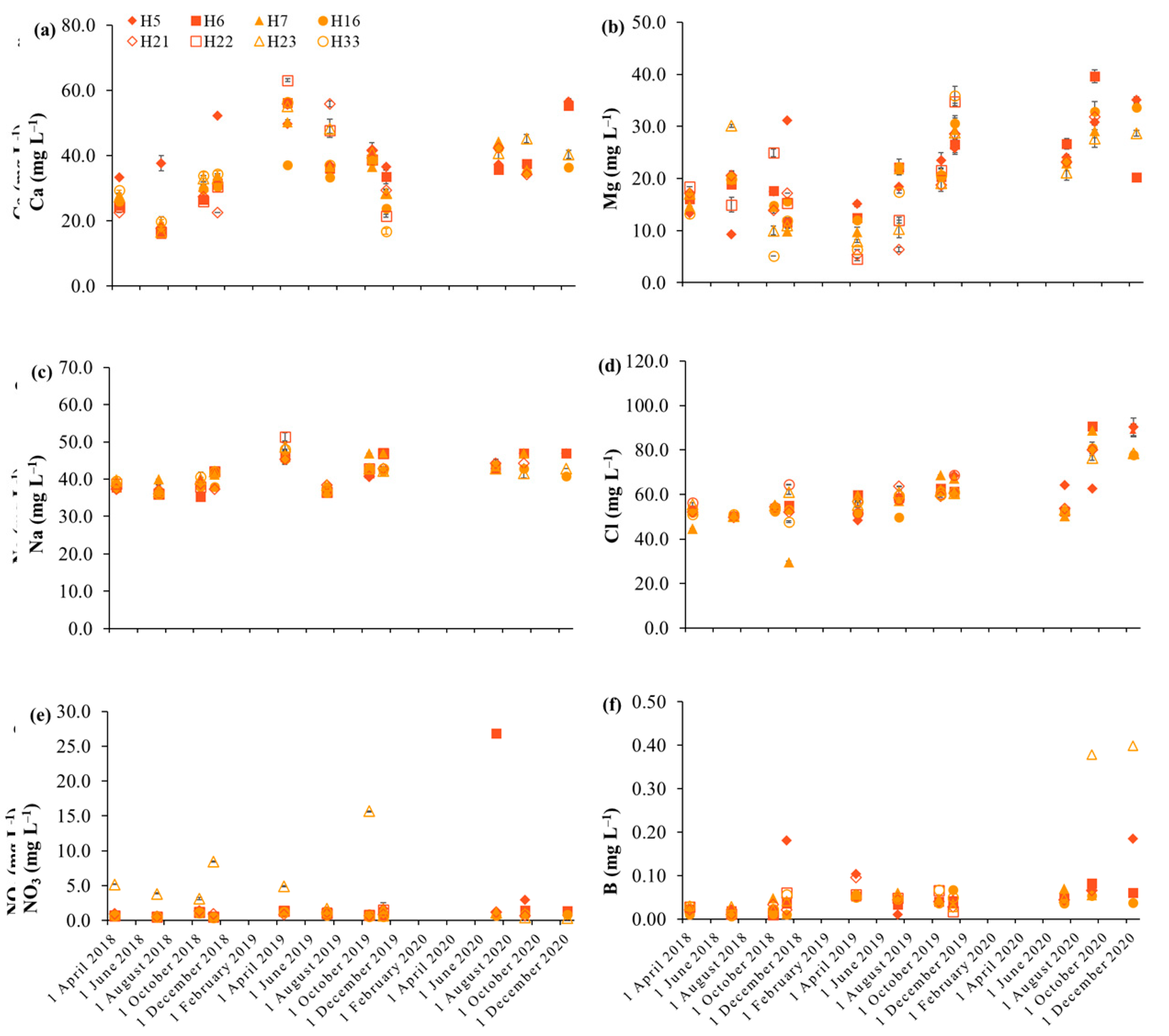
3.2. Irrigation Water Quality

The temporal and spatial variation of water physical–chemical parameters and ions was characterized by their mean and standard deviation (Figure 4 and Figure 5).
The highest ECW value was registered in H5, at the end of 2020. In general, there was a slight increase in ECW during the study period, more evident in 2019, which can be related to the drought conditions observed that year, as was confirmed by the Spearman negative correlation between this parameter and cumulative precipitation (R = −0.330; p < 0.05) (Table 2). The highest pH values occurred in H16 during the summer period of 2018 and 2019; the lowest value was registered in H5, at the end of 2020. The results highlighted that the increase in pH is negatively correlated with precipitation (R = −0.371; p < 0.05), indicating that higher frequency of dry periods may be negatively influencing some irrigation water quality parameters, such as pH and ECW.
The dominant ion in most samples was Cl, followed by Na. Overall, the order of cation abundance was Na  > Ca >   Mg  >  B. Regarding nitrate, in general, all concentrations quantified in the hydrant system were within the values stipulated for good water quality for irrigation. Exceptionally high nitrate concentrations were observed in October 2019 in H23 (15.7 mg L−1) and in June 2020 in H6 (26.7 mg L−1), classifying the water as having mild to moderate use restrictions, according to the FAO guidelines. As these values did not occur in the Lage reservoir in the same sampling period, as reported by [49], where maximum NO3 concentrations were <5 mg L−1, the concentrations may be correlated with contamination with some liquid formulation of nitrogen fertilizer (a common practice in the area), which could have occurred in the conveyance system. Despite the common origin of water, localized phenomena, like contamination or degradation within the pipeline infrastructure, may occasionally lead to deviations in water quality at the hydrant level. As reported in drinking water distribution systems, chemicals may be released from materials and equipment either by leaching due to contact with water or through corrosion in deteriorating pipes [50,51].
According to the FAO guidelines, no potential salinity problem was detected, as ECW values were persistently lower than 0.7 dS m−1 (Tables S2–S4). A slight to moderate risk of soil sodification prevailed, which should be carefully monitored, especially since the predominant soils in the study area are fine-textured and sprinkler-irrigated crops occupy a large area, potentially leading to adverse impacts on soil structure due to adsorbed Na [52]. This mild to moderate risk has already been observed at both the Alqueva and the Lage reservoirs [24,49], suggesting that the irrigation conveyance network does not significantly alter these parameters, namely, potential salinity issues and the risk of soil sodification.
Except for H16 (supplied by the Montinhos reservoir) in mid-season 2019, pH values remained within the normal range. In the study by [49], pH values measured in the Lage reservoir during 2019, the driest year, exceeded the upper limit (pH > 8.4). However, no similar trend was observed in the hydrant network; in other words, no spatial decline in pH was detected. This represents the most significant difference between the reservoirs and the hydrant system in terms of irrigation water quality assessment.

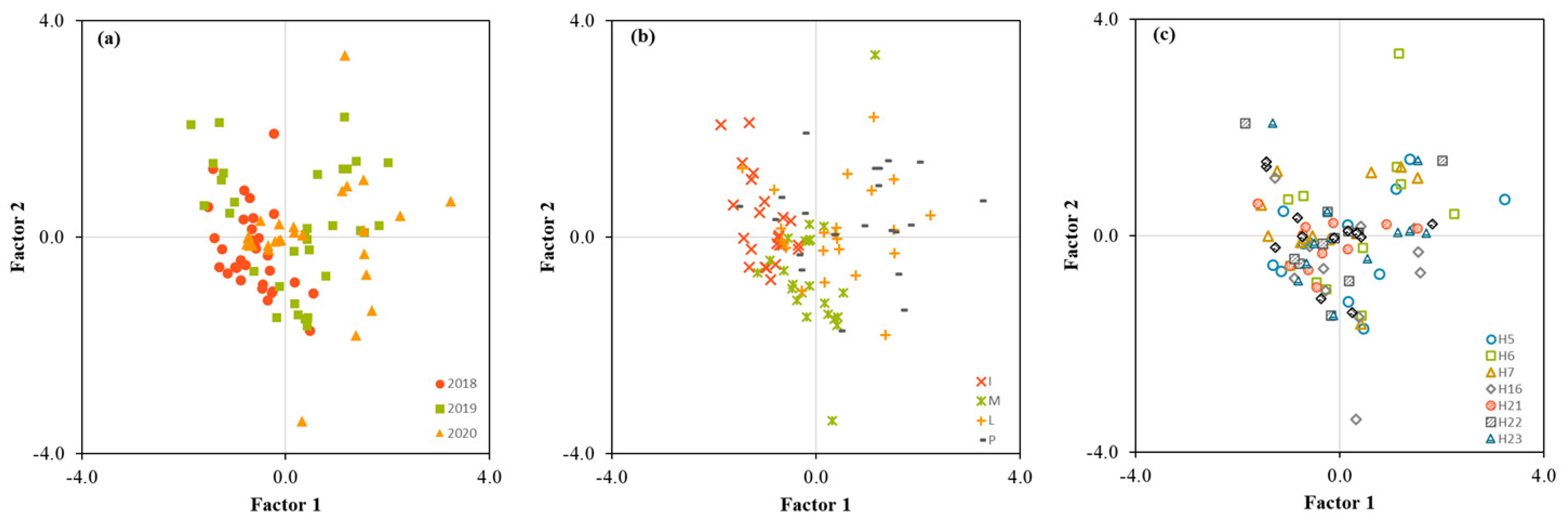
3.3. Correlation, Factor Analysis, and Cluster Analysis

To better understand the interactions between chemical parameters and meteorological conditions, exploratory analyses using multivariate statistical methods were conducted. The Spearman correlation coefficient of 11 variables, including water physical-chemical parameters (ECW, SAR, and pH), ions concentrations (Ca, Mg, Na, Cl, NO3, and B), as well as cumulative precipitation (Pcum) and cumulative reference evapotranspiration (ET0cum) until each sampling date, can be observed in Table 2.
The higher significant correlation coefficients (>|0.6|) occurred between [Ca] and [B], [Cl] and ET0cum, and SAR and [Mg], highlighting the influence of low Mg concentrations on SAR values. Other highly significant correlation coefficients (>0.5) could be found between [Mg] and ECW, between [Na] and [B], and [Cl] and ECW. Regarding correlations between meteorological variables and water physical-chemical parameters, ET0cum was significantly and positively correlated with ECW, [B], [Mg], [Na], and [Cl], pointing to an influence of high evaporative demand conditions on water salinity, and negatively correlated with SAR; Pcum was significantly and positively correlated with ET0cum, and negatively correlated with pH, ECW, [Ca], and [Na], thereby indicating that lower precipitation induced by drought is related to a decline in water quality, as highlighted by other studies on drought impacts on agricultural water quality [24,53,54]. Furthermore, the absence of strong correlations between metals, as is the case of Mg and Na (0.239) and Mg and Ca (−0.073), suggests that these chemicals may have different sources, such as anthropogenic activities (mineral fertilizers) and geologic origins through the natural weathering of carbonate and silicate rocks [55,56].
The relationships observed among variables translated into a three-factor model accounting for around 61% of the total variance in the dataset (Table 3). Factor 1 explained 29% of the variance and presented high positive loadings of ET0cum (0.691), ECW (0.703), [Cl] (0.751), and [Mg] (0.879), while a moderate positive loading was observed in [B] (0.356).
A high negative loading in Factor 1 belonged to SAR (−0.574). Therefore, Factor 1 was influenced by salinity, given the high weights of ECW, [Cl], and [Mg]. Factor 2 was responsible for explaining approximately 19% of the total variance and represented a sodicity factor as it was mainly related to [Na] (0.759) and SAR (0.666). Factor 3 represented 14% of the total variance and was positively influenced by Pcum (0.887) and ET0cum (0.318) and negatively correlated with pH (−0.693); thus, it can be considered as a climate factor.
When analyzing the score plot of cases of the first two factors, patterns of case gatherings that were year-controlled (Figure 6a) and crop irrigation stage-controlled (Figure 6b) can be recognized. The same did not apply to the grouping of cases by location (hydrants) (Figure 6c).
To clarify these groupings of cases, a CA was performed, yielding the following cluster structure (Figure 7):
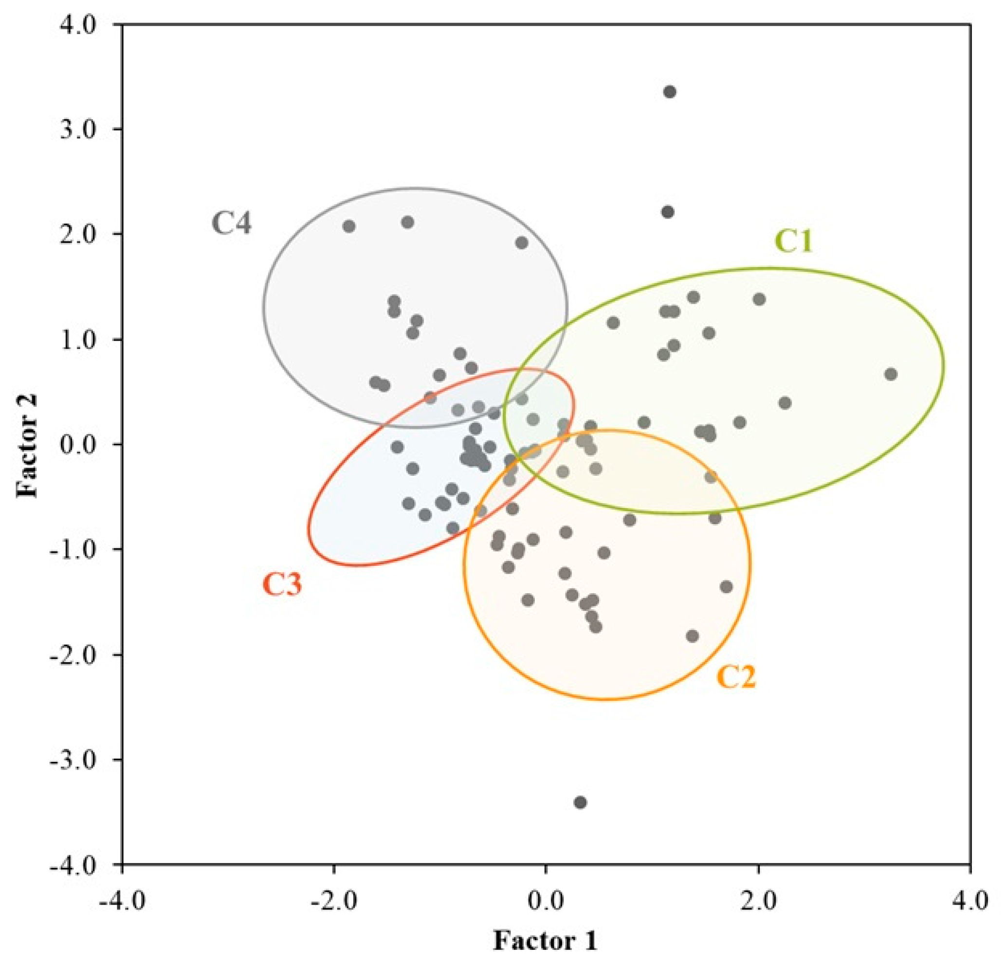
  • Cluster 1, positively related to salinity (Factor 1) and sodicity (Factor 2), was composed of 16 cases, with no samples in 2018, eight cases in 2019, and eight cases in 2020; cases were mostly of the Post-cycle (P) stage (10 samples). This structure suggests a degradation of water quality following the peak water demand by crops in Mediterranean regions, that is, a pattern of salt accumulation in water sources resulting from high evapotranspiration during summer and limited water recharge due to drought occurrence and expansion of irrigation areas [57,58].
  • Cluster 2, in the second quadrant, thus positively related to salinity, grouped 32 cases, mainly in 2019 (14 samples), with the remaining equally distributed between 2018 and 2020 cases; no samples belonged to the initial period, being mostly of the Middle (M) (13) and Late (L) (11) stages. This result reinforces the idea of the cumulative effects of evaporation and decreased freshwater recharge as the season progresses. A similar trend was reported by [59] in an irrigation district in southern Portugal, where the risk of salinity build-up was high to very high during very dry years in most fields. In wetlands located in arid/semi-arid zones, periods of higher salinity can occur as a consequence of the highly evaporative conditions and water resources’ depletion [60].
  • Cluster 3, negatively related to both salinity and sodicity, presented 32 samples, largely of 2018 (18) and 2020 (13), from the I (16) and M (9) stages of the irrigation season.
  • Cluster 4, in the 4th quadrant, grouped 13 samples of 2018 (5) and 2019 (8), the majority being of the I (8) period. Together with Cluster 4, this structure reflects the dilution effect of winter rainfall, which improves water quality at the start of the spring–summer crop cycle.
All in all, this cluster composition reveals two key effects: a drought-induced impact that intensifies salinity and sodicity levels and a seasonal influence associated with different stages of the irrigation calendar and crop cycles. Therefore, the groupings obtained confirmed the trends identified in the FA results, providing further support for the temporal patterns observed in irrigation water quality. In a study on the spatial and temporal variability of irrigation water quality in a large reservoir during a drought year, ref. [24] reported similar results, with a more time- than space-controlled pattern of sample clustering.

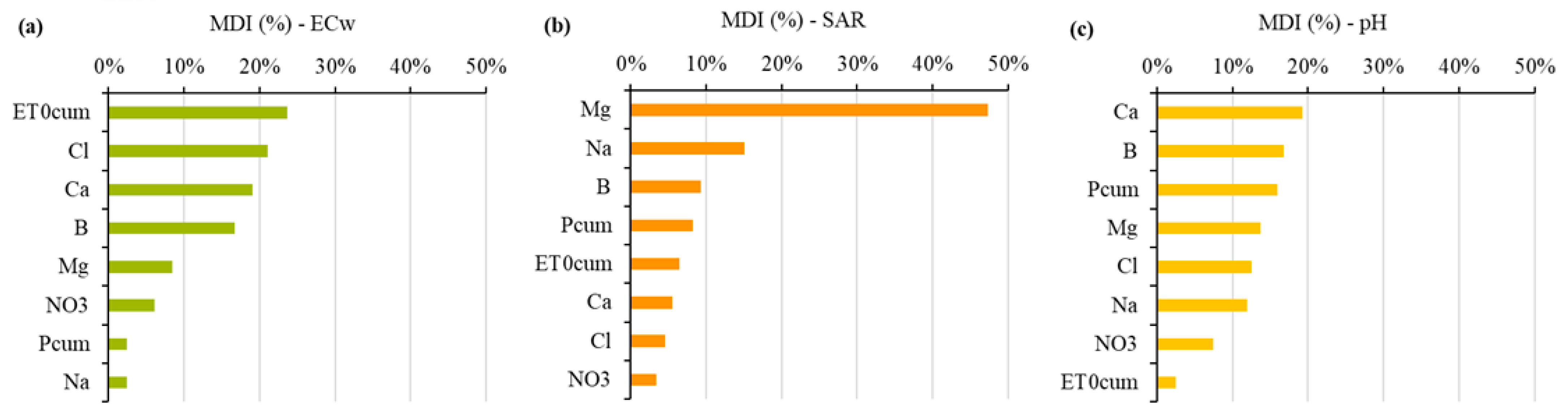
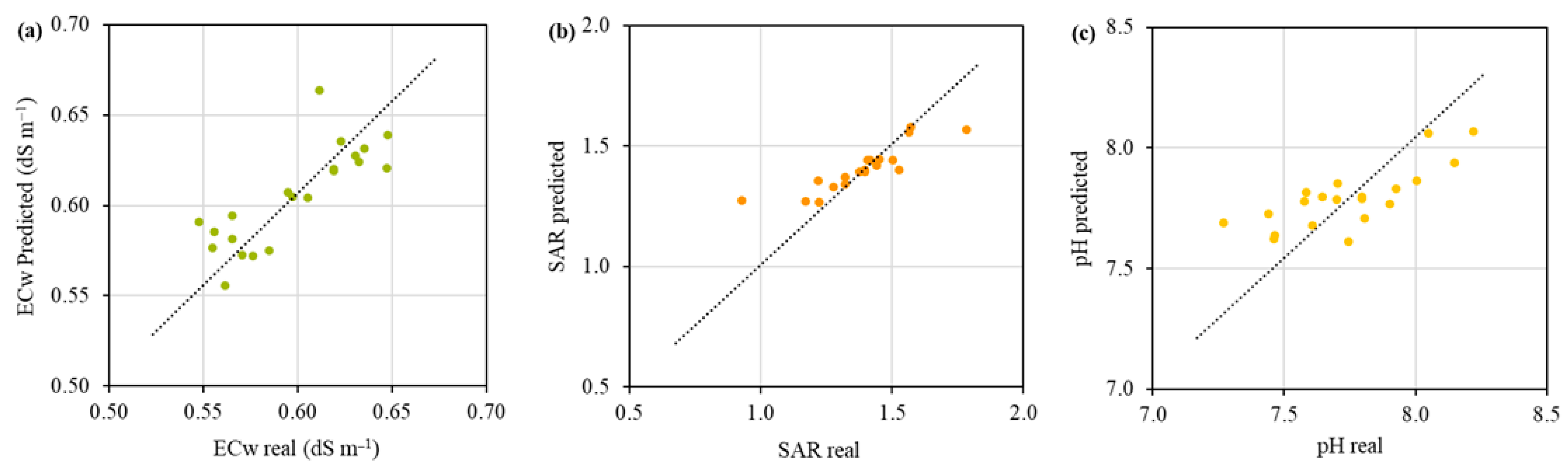
3.4. Random Forest and Gradient Boosting Models

All three RF models demonstrated satisfactory predictive performance, with particularly better results for SAR and ECW (Table 4). The model predicting SAR achieved an R2 of 0.622, a root mean square error (RMSE) of 0.106, and a mean absolute error (MAE) of 0.064, indicating a good predictive accuracy and low residual error. Similarly, the ECw model reached an R2 of 0.605, an RMSE of 0.021, and an MAE of 0.015, which supports its applicability for forecasting. The pH model presented lower predictive capacity, with R2 = 0.485, MAE = 0.146, and RMSE = 0.175, suggesting a more complex relationship between predictors and pH dynamics. All RF models exhibited low relative bias (RBIAS); namely, +1.27% for ECW, +1.46% for SAR, and +0.63% for pH, demonstrating that the predictions were not affected by systematic over- or underestimation.
In the case of GB, the model performance for predicting SAR was slightly better than in the RF regression (R2 = 0.670, RMSE = 0.099; MAE = 0.058, and RBIAS = 1.306%) but presented a lower predictive capacity both for ECw and pH. The RBIAS remained low but was generally higher than in the RF regression. Overall, the performance metrics showed that the RF was a better model to predict water quality parameters from chemical and meteorological data. These results follow [30,31], which found RF as one of the models with higher accuracy in the prediction of irrigation water quality indices like SAR, exchangeable sodium percentage (ESP), or total dissolved solids (TDS), making it a good model to be used in water quality forecasting in general but also, as our results show, under drier conditions by using different combinations of chemical and meteorological variables.
The feature importance in RF was assessed using the MDI. Results showed distinct variable contributions across the target variables (Figure 8). For ECW, the most relevant predictors were ET0cum (23.6%), Cl (21.1%), and Ca (19.1%), pointing out the influence of evapotranspiration and ion concentrations, especially chloride and calcium, on salinity levels (Figure 8a). The SAR model was largely determined by Mg (47.3%) and Na (15.1%), which was expected given their central role in SAR calculation. Pcum was one of the contributors, although having a lower weight (Figure 8b).
In the pH model, the most influential variables were Ca (19.2%), B (16.7%), and Pcum (16.0%), followed by Mg and Cl. This result suggests that the acid–base balance in irrigation water is influenced by both precipitation-related dilution and the presence of alkaline earth metals (Figure 8c).
Scatterplots of observed versus predicted values confirmed the quantitative performance of the RF models (Figure 9). Both ECW and SAR showed high correlations of 0.812 and 0.881, respectively. The pH predictions, while slightly more dispersed, are still well associated with the observed data, with a correlation of 0.772, validating the model structure for exploratory or decision support purposes.
These results indicate that the models may serve as early warning systems, allowing water management authorities and farmers to anticipate potential water quality deterioration, decline in crop productivity, and long-term degradation of soils due to salt accumulation [24].
To achieve a salt equilibrium in the soil, the influx of salt must be compensated for by salt removal, hence ensuring long-term salt sustainability in irrigated areas [61]. Therefore, the ability to predict irrigation water quality makes it easier to suggest suitable agricultural water management practices to mitigate negative effects, such as the following:
Preventive irrigation practices, such as the application of leaching fractions and suitably designed subsurface drainage systems [62,63];
Optimized irrigation timing to maintain favorable soil moisture levels [64,65];
Management of fertilizers to prevent excessive nutrient application rates, which contribute to soluble salt accumulation [66];
Selection of salt-tolerant crops [67];
Precision irrigation technologies, such as variable rate irrigation (VRI) to increase irrigation uniformity and efficiency [68];
Application of soil chemical amendments, e. g., gypsum, for sodicity control, facilitating the removal of Na ions and their replacement with Ca in the soil exchange complex [61,67].

4. Conclusions

The results in this study indicate that in small-scale hydro-agricultural irrigation systems, changes in irrigation water quality parameters within the conveyance network are not substantial and the water quality monitoring scheme can be focused on the reservoir, although safeguarding temporal scales that attend to the occurrence of extreme meteorological events and disruption of the regular trends typical of Mediterranean climate.
The dynamics of water quality for irrigation are linked to climate patterns. Dry weather during the crop growth cycle, corresponding to the irrigation campaigns, can exacerbate salinity and sodicity problems.
The RF and GB models show good predictive capability of water quality based on ion concentrations and meteorological data, with the RF model presenting, globally, better performance metrics in our study.
In agricultural water management under drought conditions, the application of ML algorithms to predict irrigation water quality based on chemical and meteorological variables can be a significant advancement, particularly in the implementation of early warning systems and the adoption of preventive measures to maintain soil health and crop yields.

Supplementary Materials

The following supporting information can be downloaded at: https://www.mdpi.com/article/10.3390/w17121783/s1 (containing Tables S1, S2, S3, and S4). Table S1. FAO guidelines for interpretation of water quality for irrigation (Ayers and Westcot 1985 [40]); Table S2. Irrigation water quality evaluation according to the FAO Guidelines—2018; Table S3. Irrigation water quality evaluation according to the FAO Guidelines—2019; Table S4 Irrigation water quality evaluation according to the FAO Guidelines—2020.

Author Contributions

Conceptualization, A.T. and P.P.; methodology, A.T.; software, P.T.; formal analysis, A.T. and P.T.; investigation, A.T., A.C., M.F., and P.P.; writing—original draft preparation, A.T.; writing—review and editing, A.T.; visualization, A.T.; supervision, P.P.; project administration, P.P.; funding acquisition, A.T. and P.P. All authors have read and agreed to the published version of the manuscript.

Funding

This work is a contribution to the projects CREATE (UIDB/06107/2023) and Geobiotec (UIDB/04035/2023), both funded by FCT—Fundação para a Ciência e a Tecnologia, Portugal, and for the FitoFarmGest Operational Group (PDR2020-101-030926). Adriana Catarino gratefully acknowledges funding from the Fundação para a Ciência e a Tecnologia, Portugal, under the PhD grant 2023.04004.BD.

Data Availability Statement

The raw data supporting the conclusions of this article will be made available by the authors on request.

Acknowledgments

During the preparation of this manuscript, the authors used Grammarly for grammar and spelling checking purposes and ChatGPT (OpenAI) for English phrasing and structure in some parts of the manuscript. The authors have reviewed and edited the output and take full responsibility for the content of this publication.

Conflicts of Interest

Author Patrícia Palma is currently serving on the Board of Directors of Águas Públicas do Alentejo (AgdA) under a public interest secondment. All authors declare that the research was conducted in the absence of any commercial or financial relationships that could be construed as a potential conflict of interest.

References

  1. Trnka, M.; Olesen, J.E.; Kersebaum, K.C.; Skjelvåg, A.O.; Eitzinger, J.; Seguin, B.; Peltonen-Sainio, P.; Rötter, R.; Iglesias, A.; Orlandini, S.; et al. Agroclimatic Conditions in Europe under Climate Change. Glob. Change Biol. 2011, 17, 2298–2318. [Google Scholar] [CrossRef]
  2. Páscoa, P.; Gouveia, C.M.; Russo, A.; Trigo, R.M. Drought Trends in the Iberian Peninsula over the Last 112 Years. Adv. Meteorol. 2017, 2017, 4653126. [Google Scholar] [CrossRef]
  3. Jones, E.; van Vliet, M.T.H. Drought Impacts on River Salinity in the Southern US: Implications for Water Scarcity. Sci. Total Environ. 2018, 644, 844–853. [Google Scholar] [CrossRef]
  4. de León, G.S.; Ramos-Leal, J.A.; Ramírez, J.M.; Almanza-Tovar, O.G. Drought and Water Quality in a Semi-Arid Area: Effects in Livestock Production, Agriculture and Use Urban. Water Resour. Manag. 2025, 39, 1605–1621. [Google Scholar] [CrossRef]
  5. Whitehead, P.G.; Wilby, R.L.; Battarbee, R.W.; Kernan, M.; Wade, A.J. A Review of the Potential Impacts of Climate Change on Surface Water Quality. Hydrol. Sci. J. 2009, 54, 101–123. [Google Scholar] [CrossRef]
  6. Delpla, I.; Jung, A.-V.; Baures, E.; Clement, M.; Thomas, O. Impacts of Climate Change on Surface Water Quality in Relation to Drinking Water Production. Environ. Int. 2009, 35, 1225–1233. [Google Scholar] [CrossRef]
  7. Cañedo-Argüelles, M.; Kefford, B.J.; Piscart, C.; Prat, N.; Schäfer, R.B.; Schulz, C.-J. Salinisation of Rivers: An Urgent Ecological Issue. Environ. Pollut. 2013, 173, 157–167. [Google Scholar] [CrossRef]
  8. Mosley, L.M. Drought Impacts on the Water Quality of Freshwater Systems; Review and Integration. Earth-Sci. Rev. 2015, 140, 203–214. [Google Scholar] [CrossRef]
  9. Phogat, V.; Cox, J.W.; Šimůnek, J. Identifying the Future Water and Salinity Risks to Irrigated Viticulture in the Murray-Darling Basin, South Australia. Agric. Water Manag. 2018, 201, 107–117. [Google Scholar] [CrossRef]
  10. Cramer, W.; Guiot, J.; Fader, M.; Garrabou, J.; Gattuso, J.-P.; Iglesias, A.; Lange, M.A.; Lionello, P.; Llasat, M.C.; Paz, S.; et al. Climate Change and Interconnected Risks to Sustainable Development in the Mediterranean. Nat. Clim. Change 2018, 8, 972–980. [Google Scholar] [CrossRef]
  11. Wenng, H.; Bechmann, M.; Krogstad, T.; Skarbøvik, E. Climate Effects on Land Management and Stream Nitrogen Concentrations in Small Agricultural Catchments in Norway. Ambio 2020, 49, 1747–1758. [Google Scholar] [CrossRef] [PubMed]
  12. Li, Z.; Fang, H. Impacts of Climate Change on Water Erosion: A Review. Earth-Sci. Rev. 2016, 163, 94–117. [Google Scholar] [CrossRef]
  13. Ramião, J.P.; Pascoal, C.; Pinto, R.; Carvalho-Santos, C. Mitigating Water Pollution in a Portuguese River Basin under Climate Change through Agricultural Sustainable Practices. Mitig. Adapt. Strateg. Glob. Change 2024, 29, 25. [Google Scholar] [CrossRef]
  14. Eswar, D.; Karuppusamy, R.; Chellamuthu, S. Drivers of Soil Salinity and Their Correlation with Climate Change. Curr. Opin. Environ. Sustain. 2021, 50, 310–318. [Google Scholar] [CrossRef]
  15. Palma, P.; Köck-Schulmeyer, M.; Alvarenga, P.; Ledo, L.; Barbosa, I.R.; López de Alda, M.; Barceló, D. Risk Assessment of Pesticides Detected in Surface Water of the Alqueva Reservoir (Guadiana Basin, Southern of Portugal). Sci. Total Environ. 2014, 488–489, 208–219. [Google Scholar] [CrossRef]
  16. Alves-Ferreira, J.; Vara, M.G.; Catarino, A.; Martins, I.; Mourinha, C.; Fabião, M.; Costa, M.J.; Barbieri, M.V.; de Alda, M.L.; Palma, P. Pesticide Water Variability and Prioritization: The First Steps towards Improving Water Management Strategies in Irrigation Hydro-Agriculture Areas. Sci. Total Environ. 2024, 917, 170304. [Google Scholar] [CrossRef]
  17. Cerdà, A.; Daliakopoulos, I.N.; Terol, E.; Novara, A.; Fatahi, Y.; Moradi, E.; Salvati, L.; Pulido, M. Long-Term Monitoring of Soil Bulk Density and Erosion Rates in Two Prunus Persica (L) Plantations under Flood Irrigation and Glyphosate Herbicide Treatment in La Ribera District, Spain. J. Environ. Manag. 2021, 282, 111965. [Google Scholar] [CrossRef] [PubMed]
  18. FAO. The State of the World’s Land and Water Resources for Food and Agriculture–Systems at Breaking Point; Main Report; Food and Agriculture Organization of the United Nations: Rome, Italy, 2022. [Google Scholar]
  19. Hillel, D.; Braimoh, A.K.; Vlek, P.L.G. Soil Degradation Under Irrigation. In Land Use and Soil Resources; Braimoh, A.K., Vlek, P.L.G., Eds.; Springer: Dordrecht, The Netherlands, 2008; pp. 101–119. ISBN 978-1-4020-6778-5. [Google Scholar]
  20. Tomaz, A.; Costa, M.J.; Coutinho, J.; Dôres, J.; Catarino, A.; Martins, I.; Mourinha, C.; Guerreiro, I.; Pereira, M.M.; Fabião, M.; et al. Applying Risk Indices to Assess and Manage Soil Salinization and Sodification in Crop Fields within a Mediterranean Hydro-Agricultural Area. Water 2021, 13, 3070. [Google Scholar] [CrossRef]
  21. Qadir, M.; Quillérou, E.; Nangia, V.; Murtaza, G.; Singh, M.; Thomas, R.J.; Drechsel, P.; Noble, A.D. Economics of Salt-Induced Land Degradation and Restoration. Nat. Resour. Forum. 2014, 38, 282–295. [Google Scholar] [CrossRef]
  22. Mateo-Sagasta, J.; Burke, J. Agriculture and Water Quality Interactions: A Global Overview; SOLAW Background Thematic Report-TR08; Food and Agriculture Organization of the United Nations: Rome, Italy, 2010. [Google Scholar]
  23. Hillel, D. Salinity Management for Sustainable Irrigation: Integrating Science, Environment, and Economics; The World Bank: Washington, DC, USA, 2000; ISBN 978-0-8213-4773-7. [Google Scholar]
  24. Tomaz, A.; Palma, P.; Fialho, S.; Lima, A.; Alvarenga, P.; Potes, M.; Salgado, R. Spatial and Temporal Dynamics of Irrigation Water Quality under Drought Conditions in a Large Reservoir in Southern Portugal. Environ. Monit. Assess. 2020, 192, 93. [Google Scholar] [CrossRef]
  25. Abbas, F.; Cai, Z.; Shoaib, M.; Iqbal, J.; Ismail, M.; Arifullah; Alrefaei, A.F.; Albeshr, M.F. Machine Learning Models for Water Quality Prediction: A Comprehensive Analysis and Uncertainty Assessment in Mirpurkhas, Sindh, Pakistan. Water 2024, 16, 941. [Google Scholar] [CrossRef]
  26. Kamel Elshaarawy, M.; Eltarabily, M.G. Machine Learning Models for Predicting Water Quality Index: Optimization and Performance Analysis for El Moghra, Egypt. Water Supply 2024, 24, 3269–3294. [Google Scholar] [CrossRef]
  27. Mohan, S.; Kumar, B.; Nejadhashemi, A.P. Integration of Machine Learning and Remote Sensing for Water Quality Monitoring and Prediction: A Review. Sustainability 2025, 17, 998. [Google Scholar] [CrossRef]
  28. Shams, M.Y.; Elshewey, A.M.; El-kenawy, E.-S.M.; Ibrahim, A.; Talaat, F.M.; Tarek, Z. Water Quality Prediction Using Machine Learning Models Based on Grid Search Method. Multimed. Tools Appl. 2024, 83, 35307–35334. [Google Scholar] [CrossRef]
  29. Alnahit, A.O.; Mishra, A.K.; Khan, A.A. Stream Water Quality Prediction Using Boosted Regression Tree and Random Forest Models. Stoch. Environ. Res. Risk Assess. 2022, 36, 2661–2680. [Google Scholar] [CrossRef]
  30. El Bilali, A.; Taleb, A.; Brouziyne, Y. Groundwater Quality Forecasting Using Machine Learning Algorithms for Irrigation Purposes. Agric. Water Manag. 2021, 245, 106625. [Google Scholar] [CrossRef]
  31. El Bilali, A.; Taleb, A. Prediction of Irrigation Water Quality Parameters Using Machine Learning Models in a Semi-Arid Environment. J. Saudi Soc. Agric. Sci. 2020, 19, 439–451. [Google Scholar] [CrossRef]
  32. Mokhtar, A.; Elbeltagi, A.; Gyasi-Agyei, Y.; Al-Ansari, N.; Abdel-Fattah, M.K. Prediction of Irrigation Water Quality Indices Based on Machine Learning and Regression Models. Appl. Water Sci. 2022, 12, 76. [Google Scholar] [CrossRef]
  33. El Bilali, A.; Taleb, A. State-of-the Art-on Irrigation Water Quality Management Using Data-Driven Methods: Practical Application, Limitations, and Prospective Directions. Phys. Chem. Earth Parts A/B/C 2024, 136, 103794. [Google Scholar] [CrossRef]
  34. IUSS Working Group WRB World Reference Base for Soil Resources 2014, Update 2015; FAO: Rome, Italy, 2014.
  35. IPMA Climate Normals-1981-2010-Beja. Available online: https://www.ipma.pt/en/oclima/normais.clima/1981-2010/#562 (accessed on 6 June 2024).
  36. COTR SAGRA-Sistema Agrometeorológico Para a Gestão Da Rega No Alentejo (Agrometeorological System for Irrigation Management in Alentejo). Available online: http://www.cotr.pt/servicos/sagranet.php (accessed on 5 January 2025).
  37. McKee, T.B.; Doesken, N.J.; Kleist, J. The Relationship of Drought Frequency and Duration to Time Scales. In Proceedings of the 8th Conference on Applied Climatology, American Meteorological Society, Anaheim, CA, USA, 17–22 January 1993; pp. 179–184. [Google Scholar]
  38. IPMA Long Series (Beja). Available online: https://www.ipma.pt/pt/oclima/series.longas/?loc=Beja&type=raw (accessed on 2 April 2025).
  39. APHA Standard Methods for the Examination of Water and Wastewater, 20th ed.; American Public Health Association, American Water Works Association and Water Environmental Federation: Washington, DC, USA, 1998.
  40. Ayers, R.S.; Westcot, D.W. Water Quality for Agriculture. In FAO Irrigation and Drainage Paper; Food and Agriculture Organization of the United Nations: Rome, Italy, 1985; ISBN 978-92-5-102263-4. [Google Scholar]
  41. Tomaz, A.; Palma, J.F.; Ramos, T.; Costa, M.N.; Rosa, E.; Santos, M.; Boteta, L.; Dôres, J.; Patanita, M. Yield, Technological Quality and Water Footprints of Wheat under Mediterranean Climate Conditions: A Field Experiment to Evaluate the Effects of Irrigation and Nitrogen Fertilization Strategies. Agric. Water Manag. 2021, 258, 107214. [Google Scholar] [CrossRef]
  42. Tomaz, A.; Martins, I.; Catarino, A.; Mourinha, C.; Dôres, J.; Fabião, M.; Boteta, L.; Coutinho, J.; Patanita, M.; Palma, P. Insights into the Spatial and Temporal Variability of Soil Attributes in Irrigated Farm Fields and Correlations with Management Practices: A Multivariate Statistical Approach. Water 2022, 14, 3216. [Google Scholar] [CrossRef]
  43. StatSoft, Inc. STATISTICA (Data Analysis Software System); Scientific Research: Wuhan, China, 2004. [Google Scholar]
  44. Breiman, L. Random Forests. Mach. Learn. 2001, 45, 5–32. [Google Scholar] [CrossRef]
  45. Friedman, J. Greedy Function Approximation: A Gradient Boosting Machine. Ann. Stat. 2000, 29, 1189–1232. [Google Scholar] [CrossRef]
  46. Sharma, A.; Jain, A.; Gupta, P.; Chowdary, V. Machine Learning Applications for Precision Agriculture: A Comprehensive Review. IEEE Access 2021, 9, 4843–4873. [Google Scholar] [CrossRef]
  47. Pedregosa, F.; Varoquaux, G.; Gramfort, A.; Michel, V.; Thirion, B.; Grisel, O.; Blondel, M.; Prettenhofer, P.; Weiss, R.; Dubourg, V.; et al. Scikit-Learn: Machine Learning in Python. J. Mach. Learn. Res. 2012, 12, 2825–2830. [Google Scholar]
  48. IPMA Drought Monitoring. Available online: https://www.ipma.pt/pt/oclima/observatorio.secas/ (accessed on 30 August 2023).
  49. Catarino, A.; Martins, I.; Mourinha, C.; Santos, J.; Tomaz, A.; Anastácio, P.; Palma, P. Water Quality Assessment of a Hydro-Agricultural Reservoir in a Mediterranean Region (Case Study—Lage Reservoir in Southern Portugal). Water 2024, 16, 514. [Google Scholar] [CrossRef]
  50. World Health Organization Water Safety in Distribution Systems; WHO Document Production Services: Geneva, Switzerland, 2014.
  51. Tong, H.; Li, Z.; Hu, X.; Xu, W.; Li, Z. Metals in Occluded Water: A New Perspective for Pollution in Drinking Water Distribution Systems. Int. J. Environ. Res. Public Health 2019, 16, 2849. [Google Scholar] [CrossRef]
  52. Tomaz, A.; Palma, P.; Fialho, S.; Lima, A.; Alvarenga, P.; Potes, M.; Costa, M.; Salgado, R. Risk Assessment of Irrigation-Related Soil Salinization and Sodification in Mediterranean Areas. Water 2020, 12, 3569. [Google Scholar] [CrossRef]
  53. do Nascimento, T.V.M.; de Oliveira, R.P.; Condesso de Melo, M.T. Impacts of Large-Scale Irrigation and Climate Change on Groundwater Quality and the Hydrological Cycle: A Case Study of the Alqueva Irrigation Scheme and the Gabros de Beja Aquifer System. Sci. Total Environ. 2024, 907, 168151. [Google Scholar] [CrossRef]
  54. Peña-Guerrero, M.D.; Nauditt, A.; Muñoz-Robles, C.; Ribbe, L.; Meza, F. Drought Impacts on Water Quality and Potential Implications for Agricultural Production in the Maipo River Basin, Central Chile. Hydrol. Sci. J. 2020, 65, 1005–1021. [Google Scholar] [CrossRef]
  55. Liu, D.; Yu, H.; Feng, H.; Gao, H.; Zhu, Y. Revealing Heavy Metal Correlations with Water Quality and Tracking Its Latent Factors by Canonical Correlation Analysis and Structural Equation Modeling in Dongjianghu Lake. Environ. Monit. Assess. 2021, 193, 717. [Google Scholar] [CrossRef]
  56. Appelo, C.A.J.; Postma, D. Geochemistry, Groundwater and Pollution, 2nd ed.; A.A. Balkema Publishers: Amsterdam, The Netherlands, 2005; ISBN 04-1536-421-3. [Google Scholar]
  57. Chartzoulakis, K.; Bertaki, M. Sustainable Water Management in Agriculture under Climate Change. Agric. Agric. Sci. Procedia 2015, 4, 88–98. [Google Scholar] [CrossRef]
  58. Huang, S.; Wortmann, M.; Duethmann, D.; Menz, C.; Shi, F.; Zhao, C.; Su, B.; Krysanova, V. Adaptation Strategies of Agriculture and Water Management to Climate Change in the Upper Tarim River Basin, NW China. Agric. Water Manag. 2018, 203, 207–224. [Google Scholar] [CrossRef]
  59. Ramos, T.B.; Darouich, H.; Oliveira, A.R.; Farzamian, M.; Monteiro, T.; Castanheira, N.; Paz, A.; Alexandre, C.; Gonçalves, M.C.; Pereira, L.S. Water Use, Soil Water Balance and Soil Salinization Risks of Mediterranean Tree Orchards in Southern Portugal under Current Climate Variability: Issues for Salinity Control and Irrigation Management. Agric. Water Manag. 2023, 283, 108319. [Google Scholar] [CrossRef]
  60. Jolly, I.D.; McEwan, K.L.; Holland, K.L. A Review of Groundwater–Surface Water Interactions in Arid/Semi-Arid Wetlands and the Consequences of Salinity for Wetland Ecology. Ecohydrology 2008, 1, 43–58. [Google Scholar] [CrossRef]
  61. Weil, R.R.; Brady, N.C. The Nature and Properties of Soils, 15th ed.; Pearson: Columbus, OH, USA, 2016; ISBN 978-0-13-325448-8. [Google Scholar]
  62. Corwin, D.L.; Rhoades, J.D.; Šimůnek, J. Leaching Requirement for Soil Salinity Control: Steady-State versus Transient Models. Agric. Water Manag. 2007, 90, 165–180. [Google Scholar] [CrossRef]
  63. Wallender, W.W.; Tanji, K.K. Agricultural Salinity Assessment and Management, 2nd ed.; American Society of Civil Engineers: Reston, VA, USA, 2011; ISBN 978-0-7844-1169-8. [Google Scholar]
  64. Hanson, B.R.; Grattan, S.R.; Fulton, A. Agricultural Salinity and Drainage. In Water Management Series Publication; University of California Irrigation Program: Davis, CA, USA, 2006. [Google Scholar]
  65. Minhas, P.S.; Ramos, T.B.; Ben-Gal, A.; Pereira, L.S. Coping with Salinity in Irrigated Agriculture: Crop Evapotranspiration and Water Management Issues. Agric. Water Manag. 2020, 227, 105832. [Google Scholar] [CrossRef]
  66. Machado, R.; Serralheiro, R. Soil Salinity: Effect on Vegetable Crop Growth. Management Practices to Prevent and Mitigate Soil Salinization. Horticulturae 2017, 3, 30. [Google Scholar] [CrossRef]
  67. Tanji, K.K.; Kielen, N.C. Agricultural Drainage Water Management in Arid and Semi-Arid Areas; FAO Irrigation and Drainage Paper; Food and Agriculture Organization of the United Nations: Rome, Italy, 2002; ISBN 978-92-5-104839-9. [Google Scholar]
  68. O’Shaughnessy, S.; Evett, S.; Colaizzi, P.; Andrade, M.; Marek, T.; Heeren, D.; Lamm; LaRue, J. Identifying Advantages and Disadvantages of Variable Rate Irrigation: An Updated Review. Appl. Eng. Agric. 2019, 35, 837–852. [Google Scholar] [CrossRef]
Figure 1. Location of the irrigation hydrants, Montinhos and Lage reservoirs, and predominant soil distribution in the hydro-agricultural area of Brinches-Enxoé, adapted from [20].
Water 17 01783 g001
Figure 2. Daily variation of (a) precipitation (P) and reference evapotranspiration (ET0), and (b) mean temperature and vapor pressure deficit (VPD).
Water 17 01783 g002
Figure 3. Monthly Standard Precipitation Index (SPI) during the study period. Droughts are identified with full yellow bars (yellow bars outlined in blue represent the end of a drought; blue bars represent monthly SPI with no drought). The table below the graph characterizes each drought for duration (months), minimum SPI value, magnitude, and intensity, according to [37].
Water 17 01783 g003
Figure 4. Temporal variation of water (a) ECW, (b) SAR, and (c) pH during the period of study (12 sampling campaigns), for each hydrant. Markers represent the mean and whiskers represent the standard deviation for three repetitions.
Water 17 01783 g004
Figure 5. Temporal variation of water ion concentrations ((a) Ca, (b) Mg, (c) Na, (d) Cl, (e) NO3, and (f) B) during the period of study (12 sampling campaigns), for each hydrant. Markers represent the mean and whiskers represent the standard deviation for three repetitions. (a) Ca, (b) Mg, (c) Na, (d) Cl, (e) NO3, and (f) B.
Water 17 01783 g005
Figure 6. Score plots of cases of the first two factors. Different shapes and colors in each graphic differentiate the year (a), stage of irrigation season: I—Initial; M—Middle; L—Late; and P—Post-cycle (b), and hydrant (c).
Water 17 01783 g006
Figure 7. Score plot of cases of the first two factors with ellipses representing significant clusters with dlink/dmax ∗ 100 < 40%.
Water 17 01783 g007
Figure 8. Feature importance of the predictor variables in the RF models, measured by the mean decrease in impurity (MDI). (a) ECW; (b) SAR; and (c) pH.
Water 17 01783 g008
Figure 9. Scatterplots of real versus predicted values of (a) ECw (r = 0.812), (b) SAR (r = 0.881), and (c) pH (r = 0.772), obtained by the RF model.
Water 17 01783 g009
Table 1. Crops in the farm plots supplied by the hydrants (coordinates between brackets), integrated with the Brinches-Enxoé hydro-agricultural area, during the period of study (2018–2020).
YearH5 (37°58′12.74″ N; 7°33′18.17″ W)H6 (37°58′22.99″ N; 7°33′26.61″ W)H7 (37°56′1.01″N; 7° 31′25.40″ W)H16 (37°59′53.28″ N; 7°32′21.02″ W)H21 (37°56′48.39″ N; 7°30′17.74″ W)H22 (37°57′12.65″ N; 7°29′21.08″ W)H23 (37°57′22.32″ N; 7°30′36.72″ W)H33 (37°57′36.03″ N; 7°29′18.35″ W)
2018Grapevine (Vitis vinifera L. Cv. ‘Aragonez)Maize (Zea mays L.)Sunflower (Helianthus annus L.)Grapevine (Vitis vinifera L. Cv. ‘Antão Vaz)Olive (Olea europaea L. Cv. ‘Cobrançosa’)Permanent Pasture ((grasses
(70%), legumes (18%) and others (12%))
Grapevine (Vitis vinifera L. Cv. ‘Antão Vaz)Alfalfa (Medicago sativa L.)
Olive (Olea europaea L. Cv. ‘Cordovil’)Sunflower (Helianthus annus L.)
2019Grapevine (Vitis vinifera L. Cv. ‘Aragonez)Sunflower (Helianthus annus L.)Arrowleaf clover (Trifolium vesiculosum Savi)Grapevine (Vitis vinifera L. Cv. ‘Antão Vaz)Olive (Olea europaea L. Cv. ‘Cobrançosa’)Permanent Pasture ((grasses (70%), legumes (18%))Grapevine (Vitis vinifera L. Cv. ‘Antão Vaz)Alfalfa (Medicago sativa L.)
Olive (Olea europaea L. Cv. ‘Cordovil’)Garlic (Allium sativum L.) + Maize (Zea mays L.)
2020Grapevine (Vitis vinifera L. Cv. ‘Aragonez)Maize (Zea mays L.)Onion (Allium cepa L.)Grapevine (Vitis vinifera L. Cv. ‘Antão Vaz)Olive (Olea europaea L. Cv. ‘Cobrançosa’)Not sownGrapevine (Vitis vinifera L. Cv. ‘Antão Vaz)Not sown
Olive (Olea europaea L. Cv. ‘Cordovil’)Sunflower (Helianthus annus L.)
Table 2. Spearman correlation matrix and heat map of water physical–chemical parameters and climate variables. Bold values are significant at p < 0.05.
PcumET0cumpHECwBCaMgNaClNO3SAR
1.0000.2940.3710.330−0.1680.3870.1050.258−0.076−0.1110.010Pcum
1.0000.1150.4010.220−0.0400.4920.2050.615−0.0400.278ET0cum
1.0000.193−0.069−0.1120.137−0.1750.071−0.183−0.171pH
<0.200 1.0000.4930.3930.5290.4260.5760.2500.454ECw
0.200–0.400 1.0000.6220.1900.5810.4440.126−0.186B
0.400–0.600 1.000−0.0730.4850.2510.1390.238Ca
>0.600 1.0000.2390.429−0.0840.624Mg
<−0.600 1.0000.4250.2280.220Na
−0.600–−0.400 1.0000.2220.282Cl
−0.400–−0.200 1.0000.106NO3
>−0.200 1.000SAR
Table 3. Factor loadings, eigenvalues, and percentage of total variance in a three-factor model of 11 observed variables. Bold values correspond to the higher absolute factor loadings of the variables in each factor.
Factor 1Factor 2Factor 3
Pcum0.099−0.1420.887
ET0cum0.6910.0900.318
pH0.076−0.289−0.693
ECw0.7030.156−0.102
B0.356−0.1350.229
Ca−0.0520.203−0.206
Mg0.879−0.1280.024
Na0.2150.759−0.096
Cl0.7510.1400.065
NO30.1330.511−0.117
SAR−0.5740.6660.144
Eigenvalues3.1602.0571.485
% Total variance28.7318.7013.50
Table 4. Performance statistics of the Random Forest (RF) and Gradient Boosting (GB) models for the prediction of ECw, SAR, and pH.
VariableModelR2RMSEMAERBIAS (%)
ECwRF0.6050.0210.0151.266
GB0.3620.0010.0172.116
SARRF0.6220.1060.0641.462
GB0.6700.0990.0581.306
pHRF0.4850.1750.1460.626
GB0.2560.0440.1610.733
Disclaimer/Publisher’s Note: The statements, opinions and data contained in all publications are solely those of the individual author(s) and contributor(s) and not of MDPI and/or the editor(s). MDPI and/or the editor(s) disclaim responsibility for any injury to people or property resulting from any ideas, methods, instructions or products referred to in the content.

