1. Introduction
Floods are natural disasters characterized by their type, volume, and duration, with their frequency rising in recent decades, sparking growing concern among scientists and decision-makers [
1]. These catastrophic events cause widespread environmental, agricultural, transportation, and infrastructure damage, resulting in fatalities and substantial economic losses [
2,
3,
4,
5]. Human activities, such as land use and climate change, have exacerbated flood risks by altering runoff responses in river catchments, intensifying flood vulnerabilities [
6]. Factors such as basin size, slope, soil structure, and urbanization further contribute to the severity of floods, as impermeable surfaces and infrastructure disrupt natural flood mitigation processes [
7,
8]. With the increasing frequency of floods, especially under the impacts of climate change, effective flood frequency analysis has become crucial for managing these disasters [
4].
The estimated flood quantiles (e.g., 50-year, 100-year discharge values) derived from frequency analysis are critical for practical engineering and flood risk management applications. These quantiles play a key role in the design of hydraulic structures like dams (typically using a 100-year return period), culverts (often designed for a 50-year flood), and bridges (commonly based on a 50- to 100-year flood) [
9]. Specifically, they determine spillway capacity and dam height, ensuring that the infrastructure can safely convey extreme flows without overtopping or structural failure. In floodplain management, flood quantiles inform zoning regulations and the delineation of high-risk areas, thereby restricting development in flood-prone zones and guiding insurance and land-use planning. Furthermore, urban drainage systems—including stormwater networks, culverts, and detention basins—rely on estimates of more frequent events (e.g., 10-year or 25-year floods) to reduce the risk of urban flooding and maintain public safety during intense rainfall events. Accurate flood frequency estimation ensures a reliable understanding of flood behavior, helping to reduce risk and protect communities. However, accurately estimating return periods for rare geophysical events such as extreme floods remains a challenge [
10].
To address this, regional flood frequency analysis (RFFA) has emerged as a widely used method, especially when data periods are unequal or records are limited or incomplete [
9]. RFFA involves pooling data from multiple sites with similar characteristics, which improves flood rate estimates and compensates for sparse data at specific sites. The RFFA process includes identifying homogeneous regions, selecting appropriate regional frequency distributions, and transferring flood characteristics from gauged to ungauged catchments. In particular, the Probability-Weighted Moment (PWM)/Generalized Extreme Value (GEV) scheme provides more reliable estimates in homogeneous regions, enhancing flood predictions and enabling better risk management strategies [
10]. Despite its advantages, RFFA must be applied cautiously, considering data uncertainties such as stationarity, correlation, and sampling variability [
11].
The L-moments method is a prominent technique for regional flood frequency analysis (RFFA) that has been successfully applied globally in regions such as Canada [
12], Norway [
13], Iran [
14], India [
15], Korea [
16], China [
17], and Turkey [
18]. Building on the Probability-Weighted Moment (PWM) method [
19], L-moments allow a more direct interpretation of flood distributions in scale and shape. This method is particularly effective for estimating distributions with more than three parameters, offering more accurate results than single-location data. The two main techniques in RFA, Annual Maximum Series (AMS) and Peak-Over-Threshold (POT) are utilized to estimate flood magnitudes based on different flood event frequencies, with AMS being beneficial for more extended return periods [
6]. L-moments significantly improve the reliability of flood discharge predictions, particularly in regions with limited data, making them essential for robust flood frequency analysis and risk management [
5].
Although the L-moments method has become popular worldwide, its application in Bangladesh is limited in various studies. Various flood frequency distributions were compared using the L-moments method without applying discordancy and heterogeneity tests, cluster analysis, or Monte Carlo simulation to estimate quantiles [
20]. The Log Pearson Type-3 (LP3) distribution was formulated as the best suited to flood frequency analysis of rivers in Bangladesh [
21], outperforming other distributions such as Log-Normal and Extreme Value Type-1 (EV1). Based on the characteristics of hydrographs, a flood index was established for the Haor area [
22]. Both Powell and Gumbel distributions were used for the Dudhkumar River, and it was observed that both these models provided a good fit, with predicted magnitudes of floods matching well with the observed magnitudes [
23]. Several approaches for the Padma River were compared, and it was concluded that Gumbel and Stochastic methods yielded the best flooding estimates, especially for extended return periods [
24]. The Hamiltonian Monte Carlo (HMC) method was used on the Generalized Extreme Value (GEV) distribution, illustrating the greater precision of HMC for extreme return periods compared to the Metropolis–Hastings algorithm [
25]. Flash floods in the northeast Haor region were analyzed, and the GEV distribution was found to be best for predicting flash flood levels and establishing new flood risk thresholds to protect Boro crops [
26]. While different approaches were adopted in these investigations, the L-moments approach was not frequently used, despite its reliability for flood frequency analysis. Our study focuses on the northeastern region of Bangladesh, a flood-prone area due to its hilly terrain, and Haors, which has large tectonic depressions that remain flooded during the monsoon but dry up post-monsoon. Flash floods occur when heavy rainfall in India’s Assam and Meghalaya regions causes floodwaters to quickly move into Bangladesh, affecting the Haor areas within hours [
27]. This rapid inundation leaves farmers with little time to harvest their Boro crops, which cover nearly 80% of the Haor areas [
28]. Flash floods have caused significant damage to crops, destroying up to 70% of them and leading to substantial economic losses [
29]. The devastating floods of 2010 and 2016 affected large areas, with the 2010 flood alone damaging 152,000 ha and causing losses worth BDT 13.18 billion [
26]. Despite existing flood control structures, such as embankments and rubber dams, the region faces serious flood risks [
30]. The 2022 flash floods, which affected over 7.2 million people and caused extensive damage, further highlight the need for better regional flood prediction and management [
31].
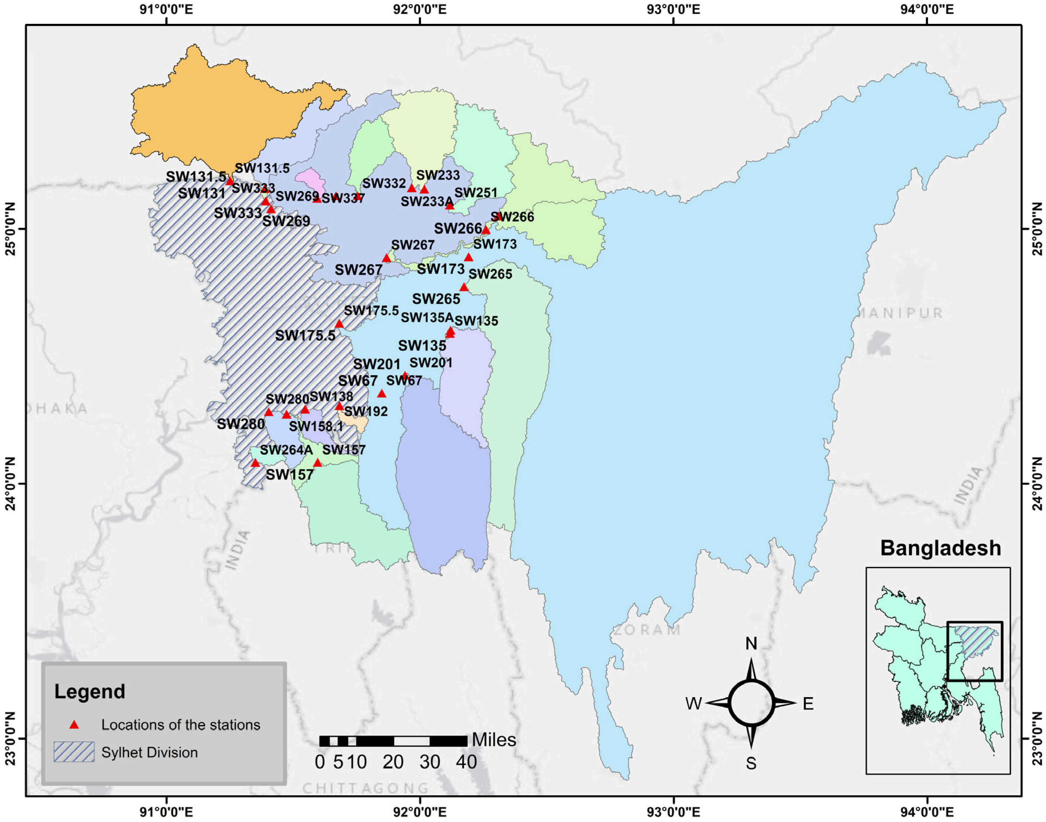
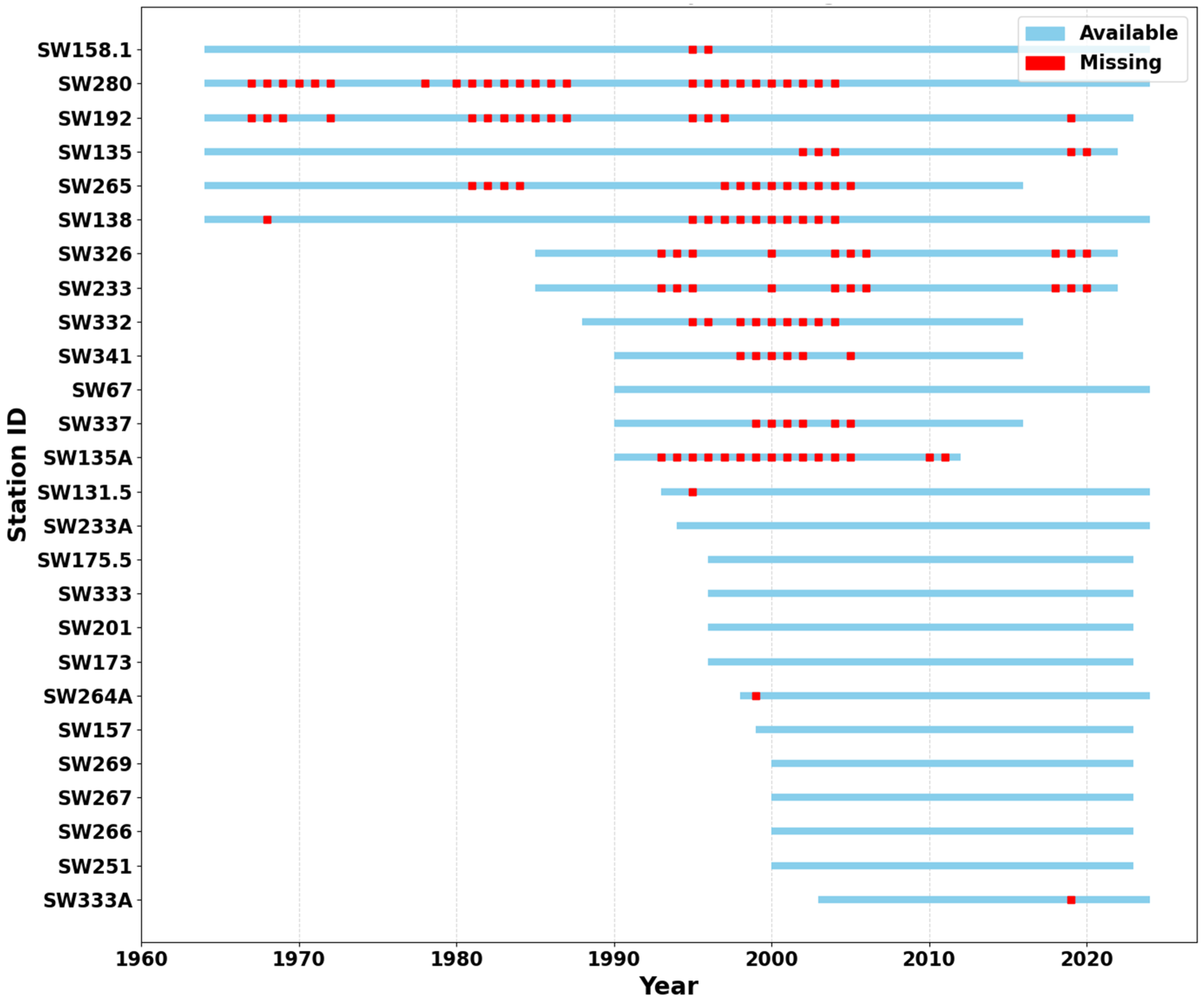
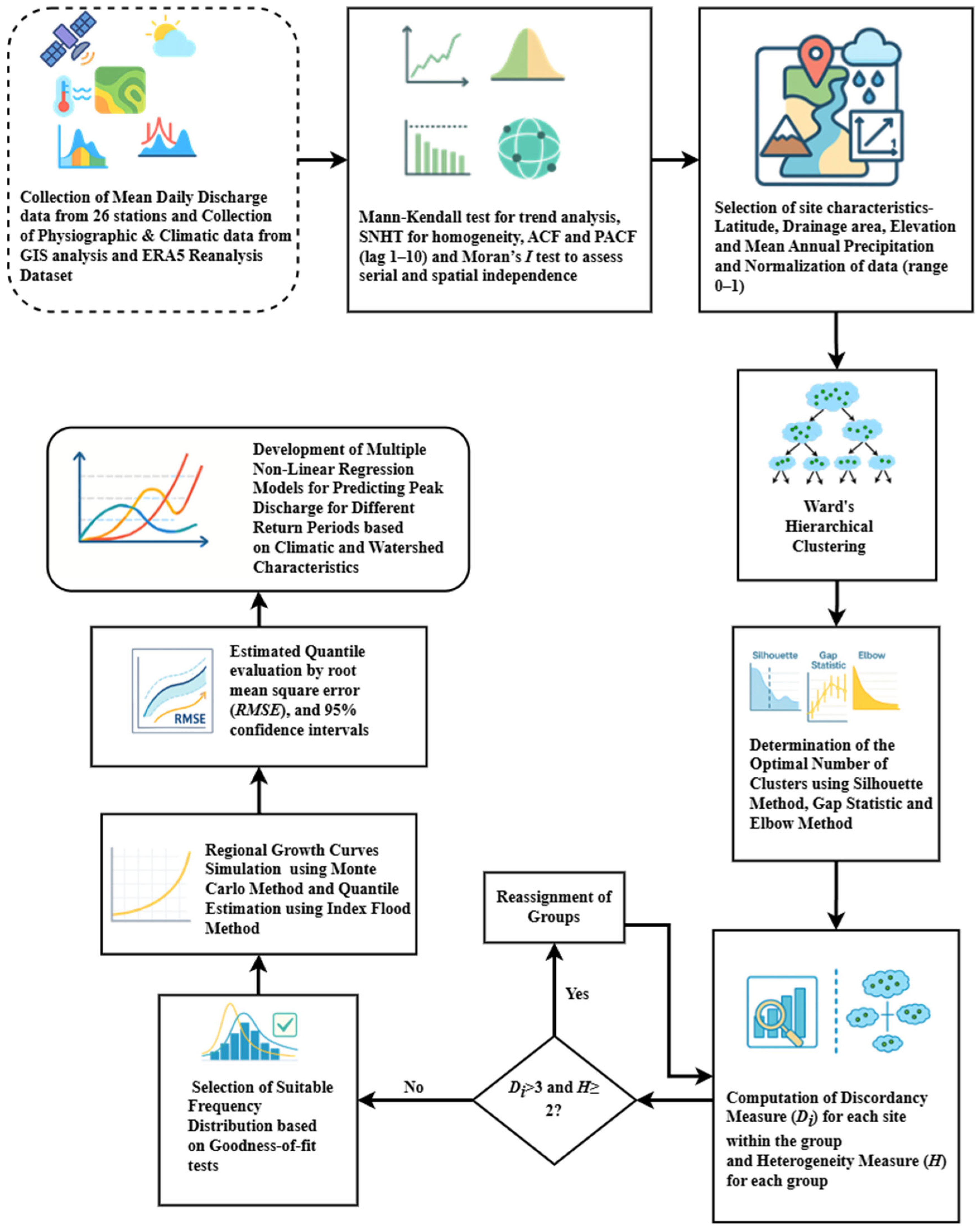
This underscores the importance of our study. This research fills a vital gap by creating and applying a physiographic–statistical framework that effectively advances classical flood frequency analysis (FFA) by combining L-moments-based regional frequency analysis and hierarchical clustering. This method is very effective for our study area since there are only 30 river discharge monitoring stations in the Sylhet Division, and data could be collected from 26 of them. Moreover, many of the discharge observation stations have short and unevenly spaced discharge records, making traditional moment-based methods less reliable. In contrast, L-moments are well-suited for such conditions, as they provide more robust and unbiased estimates even with limited or irregularly spaced data. Behind this methodological enhancement is a multi-step process starting with comprehensive data screening, including the Mann–Kendall test, Standard Normal Homogeneity Test (SNHT), autocorrelation, partial autocorrelation, and Moran’s I test, for ensuring stationarity, independence, and spatial autocorrelation of the annual peak discharge time series, followed by Ward’s hierarchical cluster algorithm based on both hydrological and physiographic watershed properties (drainage area, elevation, mean precipitation, and geographic coordinates) for delineating homogeneous regions, with cluster validity assessed using silhouette width analysis, gap statistics, and the elbow method. The proposed methodology enhances regional homogeneity testing via discordancy measures (Di statistic) for detecting anomalous stations and heterogeneity measures (H-statistics) derived from Monte Carlo simulations of synthetic regions from Kappa distributions. The selection of probability distribution is optimized by exhaustive goodness-of-fit testing by statistics between observed and simulated L-kurtosis values of six competing distributions (Generalized Logistic (GLO), Generalized Extreme Value (GEV), Generalized Pareto (GPA), Generalized Normal (GNO), Pearson Type III (PE3), Wakeby (WAK)), and the chosen distribution is also substantiated by Root Mean Square Error (RMSE) analysis and 95% confidence limits based on Monte Carlo simulations. Besides the traditional index flood methods, the study presents several predictive Multiple Non-Linear Regression (MNLR) models for different return periods that incorporate watershed-scale geomorphological predictors (stream order, basin length, elevation, etc.) and climatic predictors in an attempt to enable accurate flood quantile estimation in ungauged basins, where the performance of the model is compared using R2 (Coefficient of Determination), RMSE (Root Mean Square Error), and MAPE (Mean Absolute Percentage Error) metrics. The framework’s demonstration application in the Sylhet Division has yielded precise design flood estimates with quantified uncertainty ranges, producing vital input to climate-resilient infrastructure planning. At the same time, its techniques, particularly in cluster validation, hybrid homogeneity testing, and non-linear predictor inclusion, provide a replicable template for flood hazard estimation in similar monsoonal contexts worldwide.
3. Results
3.1. Statistical Tests for Assessing Stationarity and Independence
The Mann–Kendall test and Standard Normal Homogeneity Test (SNHT) were performed on annual peak discharge values of 26 streamflow gauging stations to detect monotonic trends, assess homogeneity, and ascertain data stationarity. If there is a trend, the data are non-stationary and unsuitable for frequency analysis without correction. From the test, it was found that only 5 out of 26 gauge stations exhibited a statistically significant trend at the 95% confidence level (for the Mann–Kendall test, a trend is considered significant if the test statistic
Z lies outside the range [−1.96, 1.96] and
p-value < 0.05), suggesting non-stationarity for annual peak discharge over time. The remaining 21 stations showed no significant trend (
p > 0.05), confirming the stationarity of the dataset and suggesting that frequency analysis can be applied directly. Six stations showed non-homogeneous behavior according to the SNHT (for the SNHT, inhomogeneity is detected if the test statistic exceeds 6.95 and
p < 0.05). As most stations exhibit no significant trend, it can be assumed that there is no consistent monotonic trend in the streamflow data at the regional level and that the data can be treated as a stationary series. The lack of substantial trends suggests that annual peak discharge variations at most stations are likely due to short-term variability rather than long-term climatic or anthropogenic changes. The test results are presented in
Table 3; marked values indicate statistically significant trends.
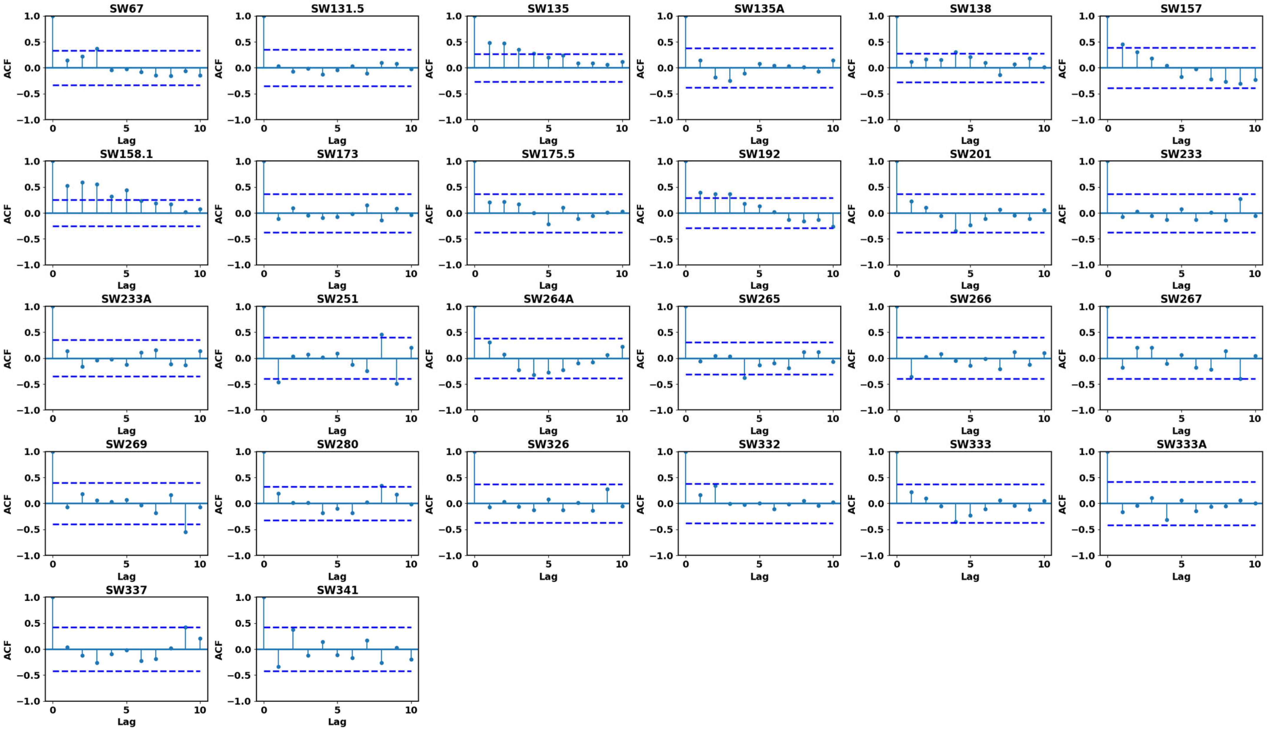
Both autocorrelation and Partial Autocorrelation Function tests were performed to determine how this year’s maximum annual discharge values related to the previous year’s. The test utilized lags of 1 to 10, and the y-axis represented the autocorrelation and partial autocorrelation coefficient while the x-axis represented lag. The 95% confidence level dashed horizontal lines indicate the limits beyond which autocorrelation and partial autocorrelation are significant at the statistical level. For the autocorrelation analysis (ACF) from lag 1 to lag 10, as illustrated in
Figure 4, it was observed that most station data do not cross the critical bounds (represented by dashed horizontal lines), indicating no significant autocorrelation in the discharge data at those lags. However, stations such as SW158.1, SW192, and SW135 showed prominent vertical spikes from lag 1 to approximately lag 5, crossing the critical limits. This suggests significant short-term autocorrelation in those stations, implying that past discharge values have a measurable influence on immediate future values. Nonetheless, the insignificance of later lags indicates that this autocorrelation diminishes over time. Most of the autocorrelation values were within boundaries since the data had no significant autocorrelation. The partial autocorrelation analysis (PACF) from lag 1 to lag 10, as illustrated in
Figure 5, revealed that the majority of stations remained within the critical bounds across most lags. Certain stations, such as SW135, SW157, SW192, and SW158.1, exhibited notable spikes from lag 1 to lag 2, with values crossing the critical limits, suggesting a significant direct correlation between consecutive years’ discharge values. Importantly, most stations showed minimal partial autocorrelation beyond lag 2, with coefficients generally remaining well within the confidence bounds for higher-order lags. This indicates that while some stations may exhibit direct year-to-year dependence, there is no significant direct relationship between discharge values separated by more than one year when intermediate effects are controlled for. The combined ACF and PACF results demonstrate that the insignificance of correlations at later lags indicates that any existing autocorrelation diminishes over time. Most autocorrelation and partial autocorrelation values were within the critical boundaries, suggesting that yearly flood values are highly independent from year to year across the majority of stations. This pattern reinforces the data independence assumptions underlying flood frequency analysis, justifying the application of standard statistical methods for extreme value analysis of annual maximum discharge data. Also, Moran’s
I analysis indicated that cross-correlation between stations was not statistically significant at the 5% level, implying the data series are spatially independent.
3.2. Initial Grouping by Cluster Analysis
Ward’s hierarchical clustering method was applied to identify homogeneous zones for regional flood frequency analysis (RFFA) using physiographic and climatic parameters, such as latitude, longitude, elevation, catchment area, and Mean Annual Precipitation. A significant drawback of using flood-based statistics to define regions is that such regions may appear statistically homogeneous but may not be hydrologically meaningful or practical for RFFA [
77]. Also, regions should not be determined solely based on physiographic characteristics, as these may overlook critical variations in hydrologic response [
78]. It is reasonable to include attributes estimated from site measurements, and they should not be strongly correlated with flood values to avoid circular reasoning [
42]. Instead, regionalization should use a combination of physical and climatic attributes that are measurable, stable, and not strongly correlated with flood magnitudes—such as catchment area, elevation, Mean Annual Precipitation, and flood seasonality indicators. This approach ensures that the regions are hydrologically meaningful and statistically sound, providing a robust foundation for applying the index flood method and estimating flood quantiles, particularly in data-scarce or ungauged basins.
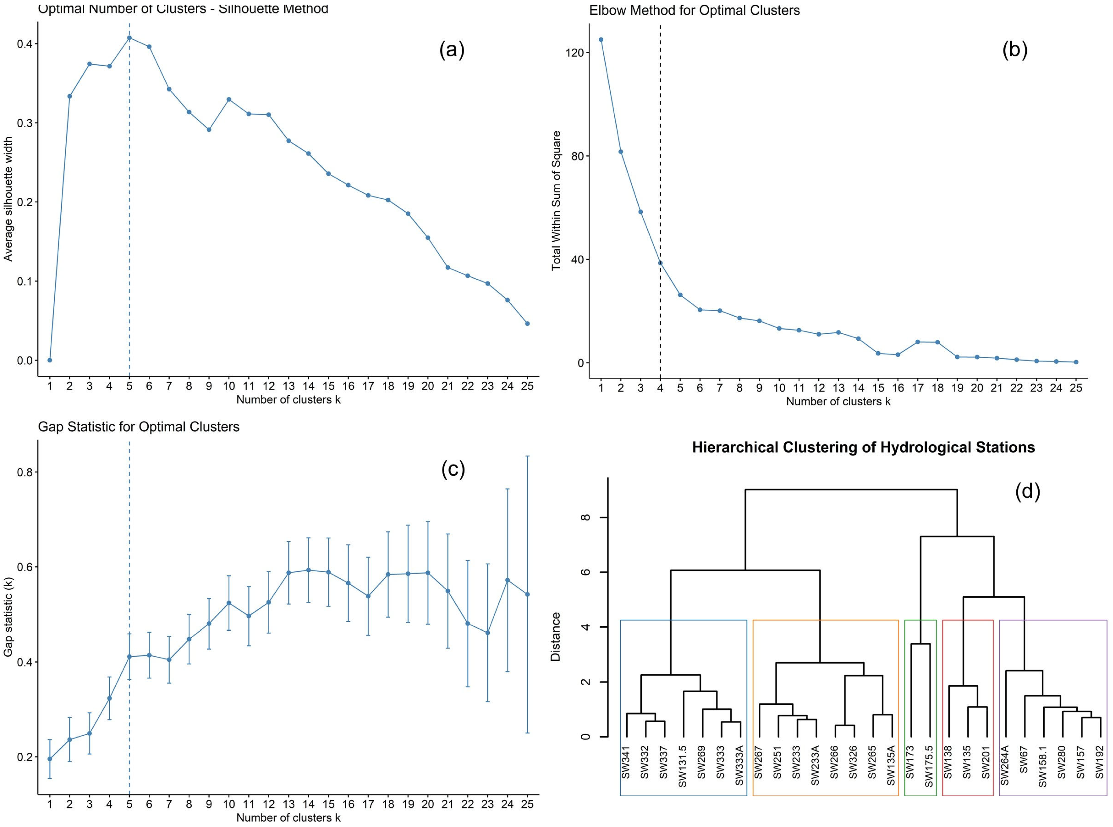
Several validation techniques were used to identify the optimal number of clusters. The gap statistic and silhouette width suggested five clusters, while the elbow method suggested four as the most suitable number. Overall, the analysis supports the delineation of four to five homogeneous regions. While initial groupings based on these features are informative, the final classification of any region should be confirmed through statistical tests of discordancy and heterogeneity. The results of Ward’s clustering method, showing the optimal number of clusters, are illustrated in the dendrogram shown in
Figure 6.
For the first group, with a critical value of 1.92 (
Dcritical = 1.92), all the included station’s discordancy values are less than this. Notably, SW337 has the least discordancy at 0.17, whereas SW269 is closest to the critical value, with a discordancy of 1.86, indicating no discordant stations in this group. Likewise, the second group, with a
Dcritical value of 2.14, shows that all stations in this group have discordancy values less than this threshold, with SW251 having the lowest discordancy at 0.34 and SW233A approaching the critical value at 1.81. For group 5, with a
Dcritical value of 1.65, the discordancy values range from a minimum of 0.67 (SW280) to a maximum of 1.36 (SW264A). For smaller subgroups like group 3 and group 4, the test measures of discordancy are always 1.00, much less than the critical values of 3.00, indicating high agreement within each group. Discordancy and heterogeneity measures are illustrated in
Table 4.
In the first group, heterogeneity values vary from 8.79 (H1) to 4.48 (H3), indicating significant differences in station streamflow characteristics. This result suggests that although the stations depict overall homogeneity with respect to discordancy, a moderate to high level of variation is observed in their streamflow characteristics, resulting in extreme differences among the stations. These sites span latitudes from 24.0834° to 25.1593°, longitudes from 91.2508° to 91.7538°, and elevations from 8 m (SW135A) to 31 m (SW131.5). Catchment areas range between 350.72 km2 (SW332) and 530 km2 (SW333A), annual precipitation ranges from 2322.55 mm (SW264A) to 4996.03 mm (SW341), and temperatures range between 18.06 °C (SW333) and 24.50 °C (SW135A).
Contrarily, the second group exhibits comparatively lower heterogeneity values, the highest being 4.53 (H1) to 2.58 (H3), pointing towards moderate variation. The stations within this group are more similar to each other than those in the first group. These sites lie between 24.0834° and 25.1624° latitude and between 91.3506° and 92.1729° longitude, with elevations from 21 m to 54 m, basin areas ranging from 726.41 km2 (SW326) to 2206.57 km2 (SW265), and annual rainfall ranging between 2521.37 mm (SW233A) and 4388.25 mm (SW333). Temperatures vary from 18.06 °C (SW333) to 24.50 °C (SW135A). The third group, composed of SW173 (24.8911° N, 92.1915° E) and SW175.5 (24.6303° N, 91.6813° E), with elevations of 59 m and 28 m, respectively, shows moderate heterogeneity with H2 = 4.30 and H1 = 2.06. This group’s catchments vary widely: 25,337.01 km2 for SW173 versus 33,855.2 km2 for SW175.5, with precipitation around 2253.36 mm (SW173) and 2360.13 mm (SW175.5) and temperatures of 20.89 °C and 21.71 °C, respectively. The fourth group exhibits excessive heterogeneity, with H-values as high as H3 = 8.78 and H1 = 6.63. These sites are spread across latitudes of 24.2930° to 24.5902° N and longitudes of 91.5465° to 92.1177° E, with basin areas of 166.96 km2 (SW138), 789.53 km2 (SW135), and 2292.71 km2 (SW201). Precipitation ranges from 2041.92 mm (SW201) to 2261.90 mm (SW138), while temperatures span 23.84 °C to 24.50 °C, indicating notable hydrological and climatic divergence. Lastly, the fifth group is distinguished by its extremely low heterogeneity, with values ranging from H1 = 1.10 to H2 = 0.08, signaling a highly homogeneous hydrological response among the stations. These sites are closely clustered between 24.0838° and 25.1301° N and between 91.3506° and 91.8489° E, with elevations from 21 m (SW264A) to 25 m (SW157). Catchment areas are generally modest, between 61.29 km2 (SW192) and 1142.76 km2 (SW157). Rainfall is also fairly uniform, ranging from 2199.38 mm (SW157) to 4474.48 mm (SW341), and temperature values are consistently between 24.12 °C and 24.55 °C.
In general, although most groups are homogeneous in terms of discordancy (Di < Dcritical), the measures of heterogeneity () indicate a range of variability within the groups. There are groups with high heterogeneity (groups 1 and 4) and groups with minimal variation (group 5).
3.3. Formation of Homogeneous Regions by Discordancy and Heterogeneity Measures
As shown in
Table 4, although the discordancy levels were mostly acceptable, the initially high heterogeneity among most groups required an intensive refinement process to achieve more homogeneous regional groupings of the initially clustered homogeneous groups; the final grouping resulted in four well-defined regions exhibiting acceptable homogeneity. This process involved a series of iterations, where the stations were regrouped based on heterogeneity checks and discordancy assessments. In each iteration, the groups were rearranged carefully, and the discordancy and heterogeneity values were recalculated to ensure all regions met the specified standards (i.e.,
Di <
Dcritical and
), as shown in
Table 5.
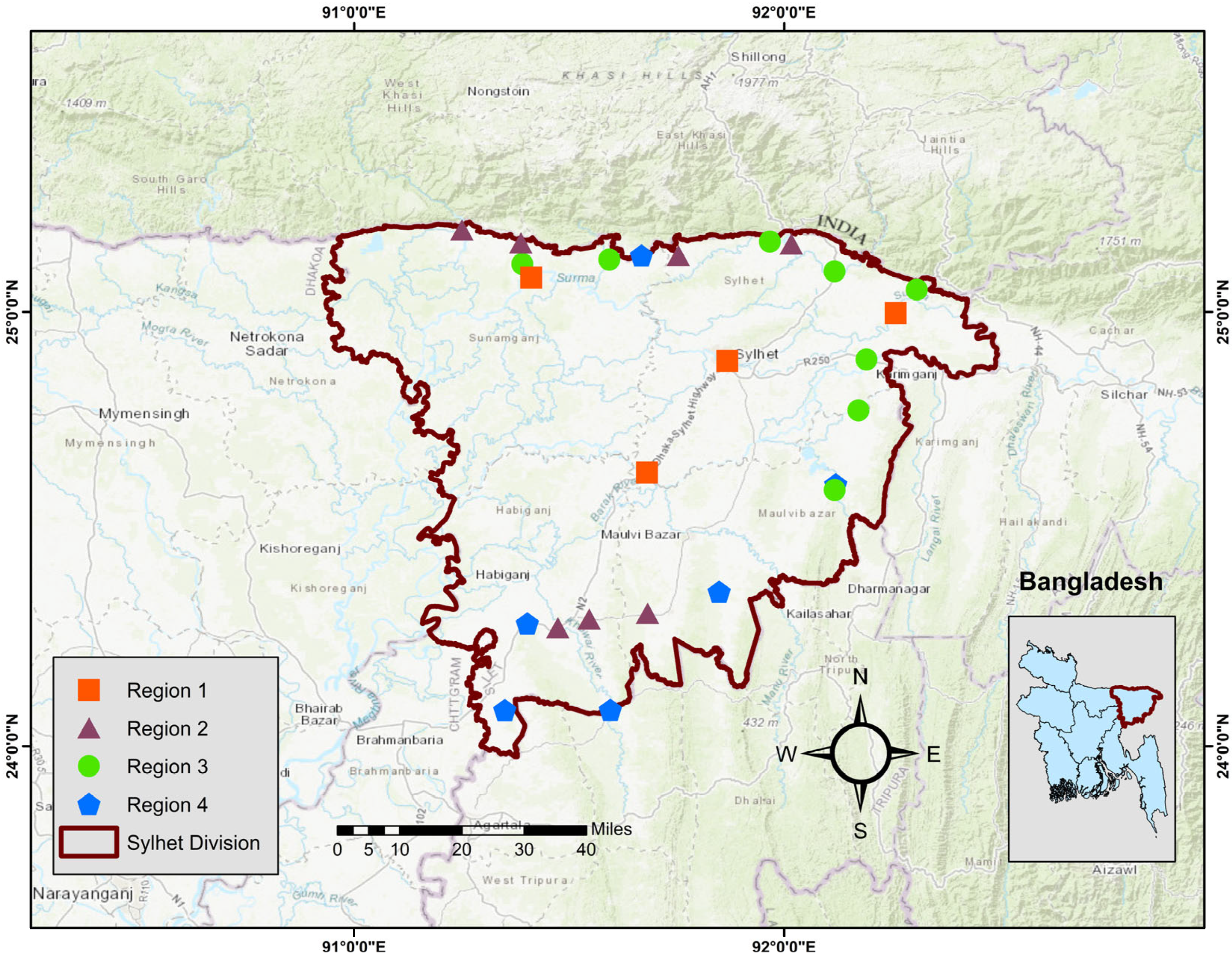
As shown in
Table 5, region 1 consists of four stations: SW175.5, SW266, SW267, and SW269. These stations are geographically confined to a small region and exhibit similar hydrological characteristics. Region 2 comprises seven stations: SW131.5, SW138, SW158.1, SW192, SW332, SW233A, and SW333A. Although these stations are reasonably dispersed across the study area, they share similar runoff characteristics. Region 3 consists of eight stations: SW135, SW173, SW233, SW251, SW265, SW326, SW337, and SW333. This region encompasses a hydrologically heterogeneous region, including upstream and downstream basins, resulting in substantial elevation and basin area variation. Region 4 comprises six stations: SW67, SW157, SW280, SW341, SW135A, and SW264A. Lastly, SW201 could not be assigned to any group and was therefore omitted, as including SW201 in any region caused the discordancy (
Di) and heterogeneity (
H) values to exceed their acceptable thresholds, violating the grouping criteria (i.e.,
Di <
Dcritical and
). The final arrangement, as outlined in the table, is the best categorization, in which there were no discordant stations, except for station SW333 of region 3, which slightly surpassed the critical discordancy (
Di (2.26) >
Dcritical (2.14)) value but passed the heterogeneity test. The location of all four homogeneous regions is shown in
Figure 7.
3.4. Goodness-of-Fit Test and Selection of the Best Parent Distribution, Along with the Derivation of the Growth Curve for Each Homogeneous Region
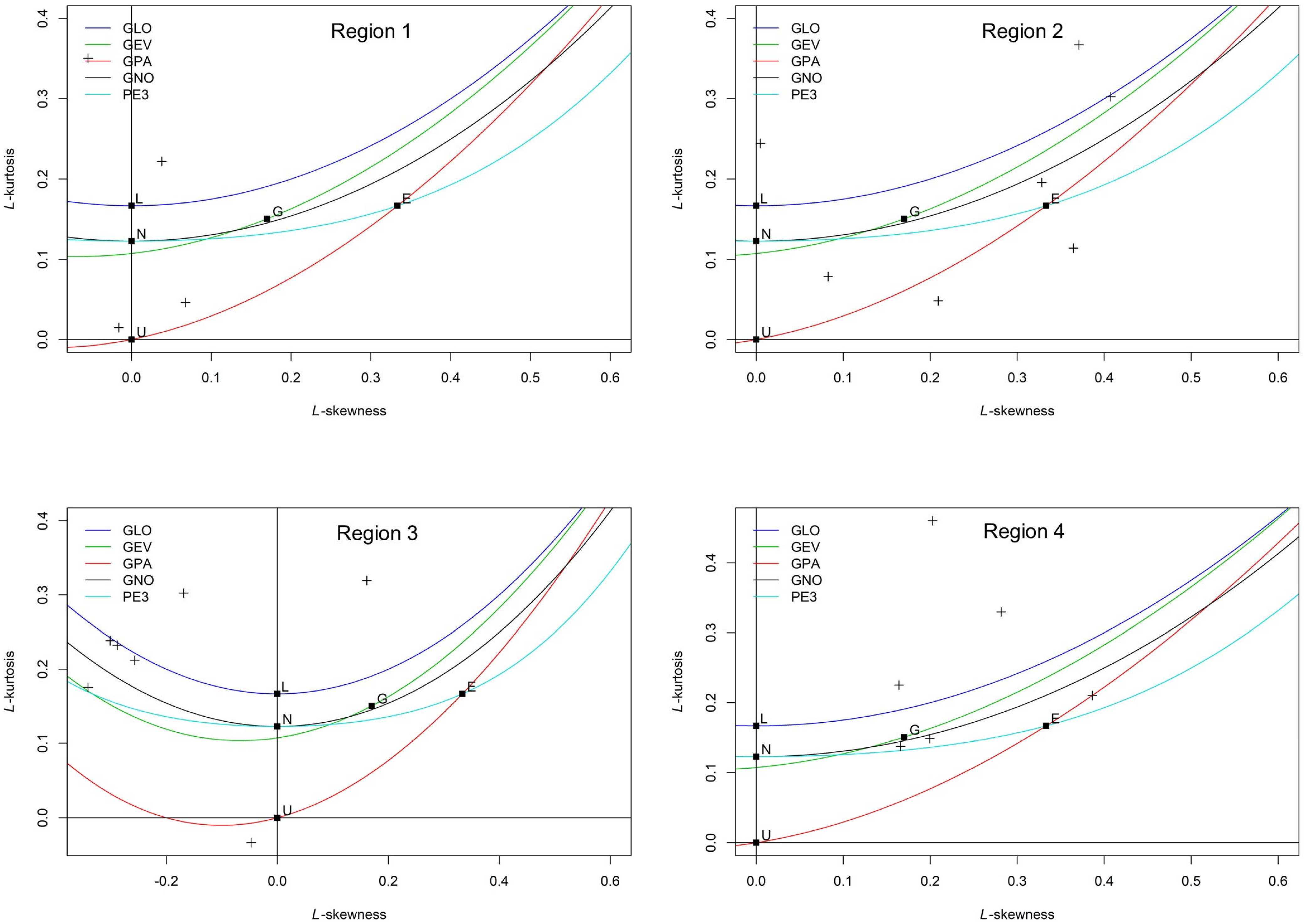
We created L-moment diagrams to assess the probability distributions in the study area.
Figure 8 presents a comparison between the observed data and theoretical distribution patterns. However, finding a suitable probability distribution to fit most of the observed regional data is challenging.
The variation in hydrological conditions among sites results in wide-ranging variation in L-moment characteristic values. The single distribution, thus, does not always yield the optimum possible fit for every site. Whereas some datasets perform reasonably well when fitted against the Generalized Extreme Value (GEV) or Pearson Type III distributions, others exhibit extreme disagreement. This suggests that a flexible or site-specific approach to distribution fitting may be necessary to represent the underlying hydrological processes in the region accurately.
To identify suitable parent distributions for each homogeneous region, the good-ness-of-fit statistic
was determined for several candidate distributions: Generalized Logistic (GLO), Generalized Extreme Value (GEV), Generalized Normal (GNO), Generalized Pareto (GPA), and Pearson Type III (PE3). In cases where multiple
values fell within the acceptable range (
) for a region, a simulation-based approach was adopted to select the most robust distribution [
42]. Any distribution with a calculated value not exceeding this threshold was considered a potential candidate, as denoted in
Table 6.
Table 7 shows the estimates of the regional parameters for L-moments for the suitable probability distribution.
For regions 1, 2, and 4, more than one distribution passed the critical value in one region. To further narrow down the selection and determine the best distribution, we compared the Root Mean Square Error (RMSE) values and 95% confidence intervals of the regional growth curves for each qualifying distribution. For example, in region 1, the GLO, GEV, GNO, and PE3 distributions all passed the criteria set by the critical value test. Among these distributions, GLO showed the narrowest 95% confidence intervals and lowest RMSE value, particularly for the 50- and 100-year return periods, indicating higher accuracy and less uncertainty in extreme value estimation. Therefore, GLO was selected as the most appropriate distribution for region 1. The same procedure was followed for regions 2, 3, and 4.
Although more than one distribution passed the initial critical value threshold, GLO always had the lowest
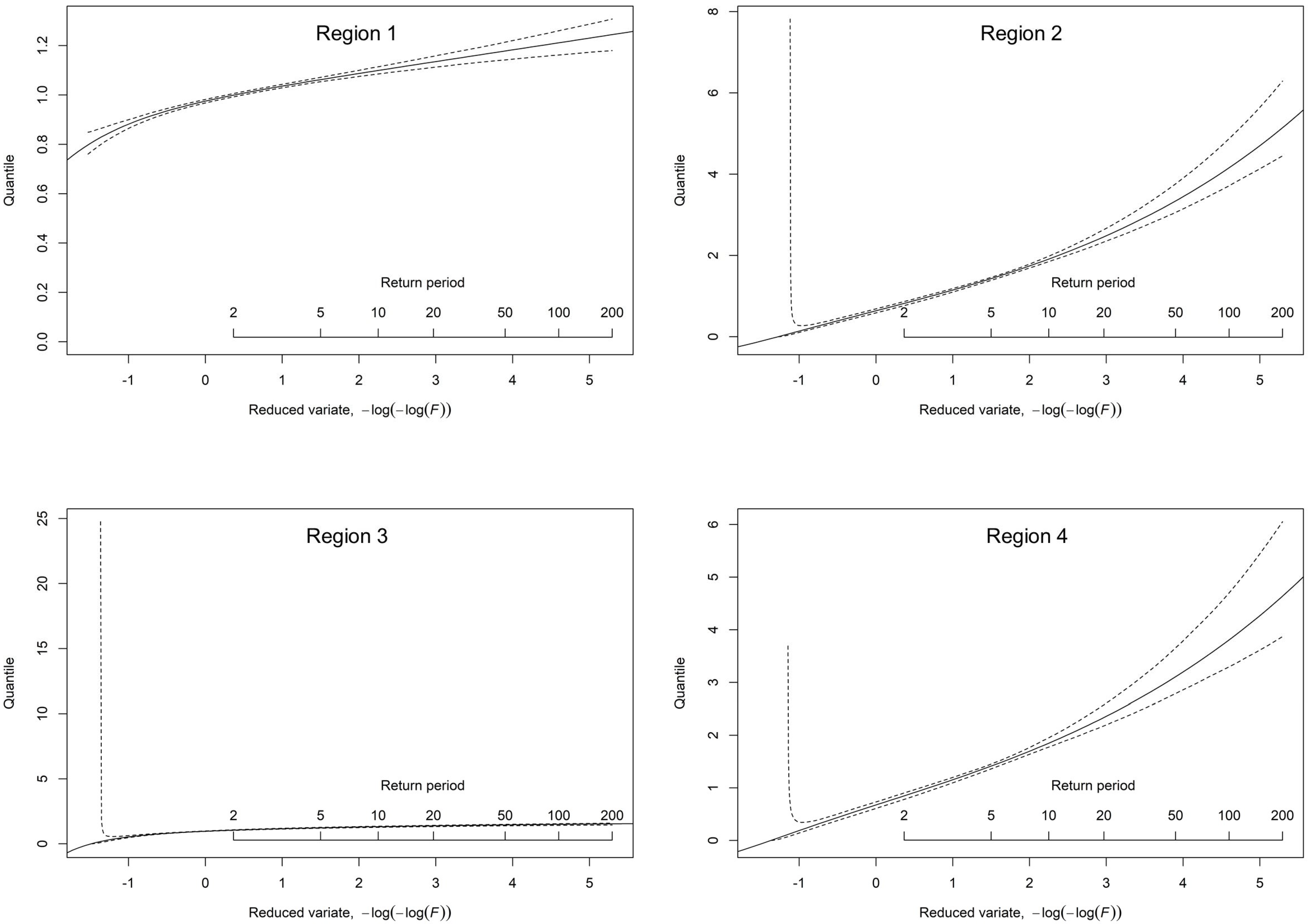
RMSE or the smallest and most consistent 95% error bounds for all significant return periods. For this reason, GLO was selected as the best fit for all four regions. Moreover, regional growth curves with 95% error bounds for GLO distribution are given in
Figure 9. As presented in
Table 8, quantile estimates across 50-, 100-, 200-, and 1000-year return periods (f = 0.98, 0.99, 0.995, 0.999) reveal significant regional variations in precision and uncertainty. Region 1 demonstrates exceptional stability, with consistently low
RMSEs (0.0243 for 50-year, 0.0323 for 100-year, 0.0424 for 200-year, and 0.0740 for 1000-year) and narrow confidence bounds (1.1337–1.2077 for 50-year, 1.1507–1.2426 for 100-year, 1.1653–1.2774 for 200-year, and 1.1884–1.3575 for 1000-year), indicating highly reliable predictions across all return periods. Region 2 shows dramatically increasing uncertainty, with
RMSEs surging from 0.4621 (50-year) to 0.7097 (100-year), 1.0853 (200-year), and 2.7769 (1000-year), accompanied by rapidly expanding bounds (2.6369–3.9559 to 3.0998–4.8887 to 3.6054–5.9676 to 4.9954–9.1964), highlighting difficulties in extreme value estimation.
Region 3 maintains moderate precision throughout, with
RMSEs ranging from 0.1204 to 0.2068 and bounds (1.2560–1.5997 to 1.2679–1.6481 to 1.2759–1.6885 to 1.2813–1.7572) that suggest reasonable reliability even for rare events. Region 4 exhibits concerning variability, particularly for more extended return periods, with
RMSEs climbing from 0.3499 (50-year) to 0.5461 (100-year), 0.8468 (200-year), and 2.1913 (1000-year) and bounds widening significantly (2.5513–3.5651 to 2.9598–4.3449 to 3.4013–5.2387 to 4.5394–7.8847). These patterns underscore critical regional differences in extreme value behavior, with regions 1 and 3 offering relatively stable estimates suitable for precise risk assessment. In contrast, region 2 and region 4 require cautious interpretation and potentially more conservative approaches in engineering and planning applications due to their pronounced uncertainty, especially for 200-year and 1000-year events. Regional flood quantile estimates with associated uncertainty bands across different return periods are plotted in
Figure 10.
The log-log return period plot in
Figure 10 shows that the regional
q(
F) curves both intersect and diverge at different return periods, highlighting important hydrological differences among the regions. At lower return periods (around 2 to 5 years), region 3 initially exhibits higher quantile values compared to region 2 and region 4, indicating a greater frequency of moderate events; however, as the return period increases, the curves for regions 2 and 4 rise more steeply and overtake region 3, suggesting a higher magnitude of extreme events in those regions. This crossing pattern implies that the severity of events relative to other regions shifts depending on the frequency of occurrence. Beyond approximately 10 to 20 years, the curves begin to diverge significantly—regions 2 and 4 continue to rise rapidly, while regions 1 and 3 remain relatively flat, indicating lower susceptibility to rare, extreme events. This divergence at higher return periods underscores the need for region-specific planning, as some areas face far greater risks of severe hydrological extremes than others.
3.5. Regional Flood Frequency Relationship for Ungauged Catchments
To estimate the T-year return period flood at a site, the mean annual peak flow must first be determined. However, due to the lack of observed flow data, this site-specific mean cannot be calculated for ungauged catchments. In such cases, developing a relationship between the mean annual peak flows of gauged catchments in the region and their corresponding physiographic and climatic characteristics becomes essential. This regional relationship can then estimate ungauged sites’ mean annual peak flow at different return periods.
At-site annual maximum discharge values for various return periods were derived by multiplying the regional growth curve values by the mean annual peak discharge specific to each site.
Table 9 provides the estimated maximum flood discharges corresponding to each gauging station, reflecting the expected discharge levels for different return intervals. Key geomorphological parameters were extracted using Geographic Information System (GIS) software (ArcGIS Desktop 10.8) and presented in
Table 10. These include Total Stream Length and Number of Streams, representing the cumulative length and count of stream segments within the watershed. Additional attributes such as Perimeter, Main Channel Length, Maximum Basin Length, and Maximum Stream Order describe the watershed boundary, principal flow path, longest dimension, and drainage network complexity—factors that significantly influence hydrological response and flood behavior.
Equations for the prediction of peak flood discharge for various return periods were developed using the Multiple Non-Linear Regression (MNLR) model, based on watershed and climatic variables, as shown in
Table 11. These equations incorporate key parameters such as area (km
2) (
A), elevation (m) (
E), Total Stream Length (km) (
TSL), Number of Streams (
NS), Perimeter (km) (
P), Main Channel Length (km) (
MCL), Maximum Basin Length (km) (
MBL), Maximum Stream Order (
MSO), Mean Annual Precipitation (mm) (
MAP), and Mean Annual Temperature (°C) (
MAT) for estimating peak discharge.
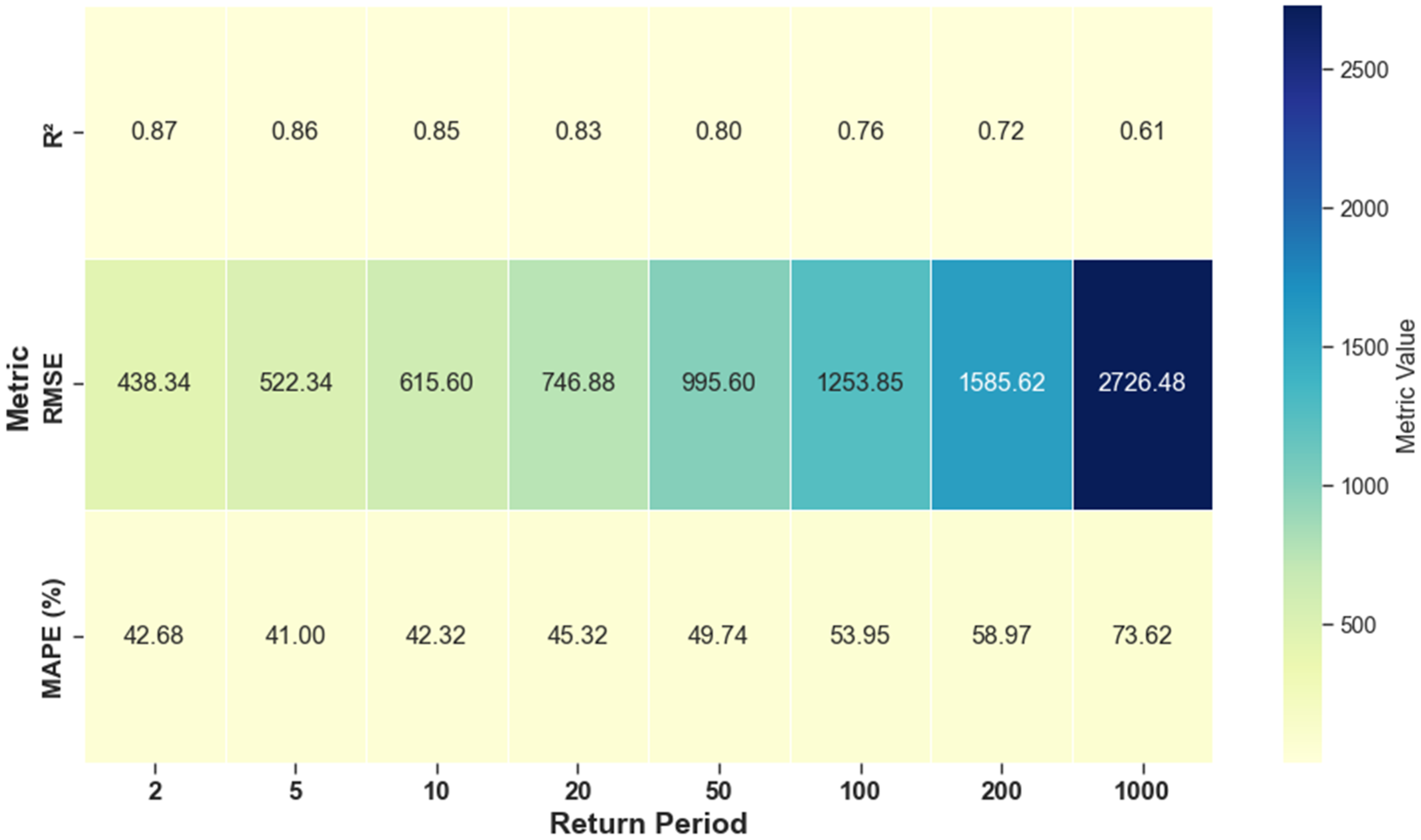
The performance of the models, as indicated by the Coefficient of Determination (
R2), Root Mean Square Error (
RMSE), and Mean Absolute Percentage Error (
MAPE), demonstrates strong predictive accuracy, as illustrated in
Figure 11, particularly for lower return periods. Predictive reliability decreases with increasing return periods, reflecting growing uncertainty in extreme flood estimation.
It should be noted that the equations are only applicable to the four homogeneous regions created earlier and are intended for use in both gauged and ungauged catchments within those regions. As the return period increases, predictive performance weakens, evidenced by the decline in
R2 values and the increase in both
RMSE and
MAPE (
Table 11). The pattern shows the growing uncertainty and complexity in quantifying long-return-period extreme flood events. Lower values of
R2 and larger errors at longer return periods highlight model limitations in reliability for extreme floods and imply large variance. Hence, these uncertainties and associated errors must be cautiously quantified while utilizing the models, especially for long-return-period events.
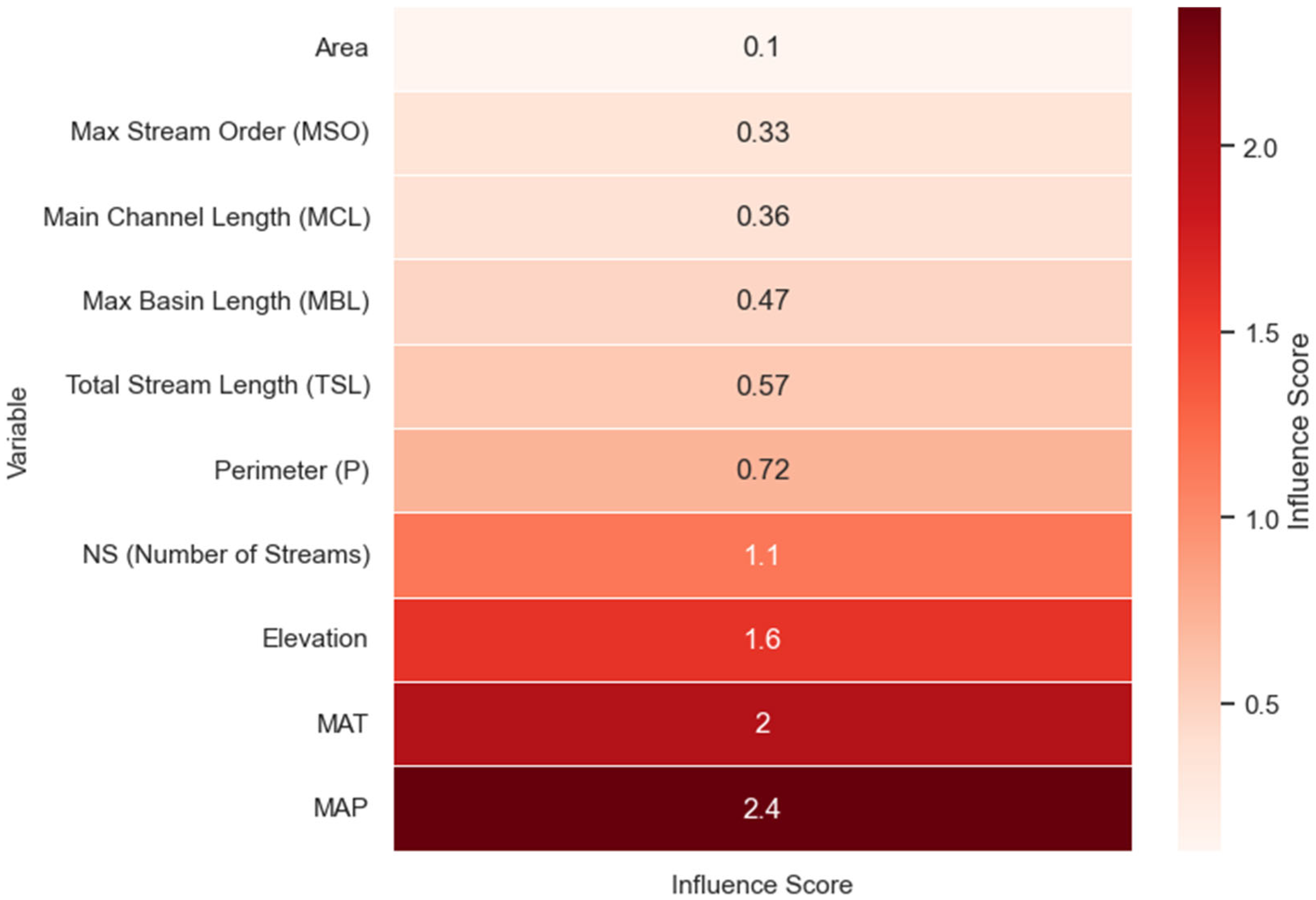
Figure 12 illustrates the average impact of various physiographic and climatic variables on peak discharge, based on the absolute values of exponents in Multiple Non-Linear Regression equations. Among the variables considered, Mean Annual Precipitation and Mean Annual Temperature exhibit the largest effect values, 2.4 and 2.0, respectively, indicating their dominant control on peak discharge. Elevation (1.6), Number of Streams (1.1), and Perimeter (0.72) also reflect comparatively high control. Geometric parameters such as area (0.1), Maximum Stream Order (0.33), and Main Channel Length (0.36) exhibit lower values of influence, reflecting comparatively less impact on peak flow generation. The trend reveals the significant contribution of climatic and topographic factors over the simple morphometric parameters in the formation of flood peaks.
4. Discussion
This study presents a comprehensive framework for regional flood frequency analysis (RFFA) using L-moments in northeastern Bangladesh, addressing critical gaps in existing methodologies by integrating rigorous data screening via the Mann–Kendall test, the Standard Normal Homogeneity Test, autocorrelation, partial autocorrelation, and Moran’s
I test to ensure stationarity and spatial independence—an essential step often overlooked [
20,
21,
23,
24,
25]. This contrasts with earlier assumptions that flood flows strictly follow specific probability distributions, and the current study highlights the importance of flexible, region-specific approaches in flood frequency analysis. In many cases, the scale and shape parameters of the distributions were estimated using the method of moments. A key finding from several studies conducted in Bangladesh is the superiority of the Generalized Logistic (GLO) distribution over traditionally used distributions such as Log-Normal (both two-parameter (LN2) and three-parameter (LN3)), Extreme Value Type-I (EV1), and Log Pearson Type III (LP3) distributions [
21]; the Gumbel and Powell method [
23]; and Gumbel, Powell, and Ven Te Chow and Stochastic methods [
24]. The GLO distribution demonstrated narrower confidence intervals and lower
RMSE, providing more reliable quantile estimates across all return periods. The study enhances the initial regional grouping by applying Ward’s hierarchical clustering algorithm, with cluster validity evaluated using silhouette width analysis, gap statistics, and the elbow method. The study strengthens the analysis by incorporating both discordancy measures (
Di statistic) and heterogeneity measures (
H-statistics), which were not employed in the previous approach in Bangladesh [
20]. For ungauged basins, Multiple Non-Linear Regression (MNLR) models incorporating geomorphologic and climatic predictors—previously unexplored in the context of Bangladesh—achieved strong performance with
R2 = 0.61–0.87 for 2- to 100-year floods. Although uncertainty increased for extreme events (
MAPE = 41–74%,
RMSE up to 2726 m
3/s for 1000-year floods), the results are consistent with findings from similar studies conducted globally [
12]. In contrast, some previous studies outside Bangladesh [
16] used only a single predictive variable (area), whereas this study employs 10 geomorphologic and climatic variables to improve prediction accuracy.

 ,
, 


