
A Hierarchical Water Supply–Demand Regulation Model Coupling System Dynamics and Feedback Control Mechanisms: A Case Study in Wu’an City, China


Abstract
1. Introduction
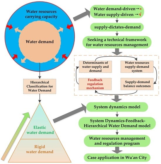
2. Methodology
2.1. SD Model
2.2. Feedback Regulation Mechanism
2.3. Method of Hierarchical Classification for Water Demand
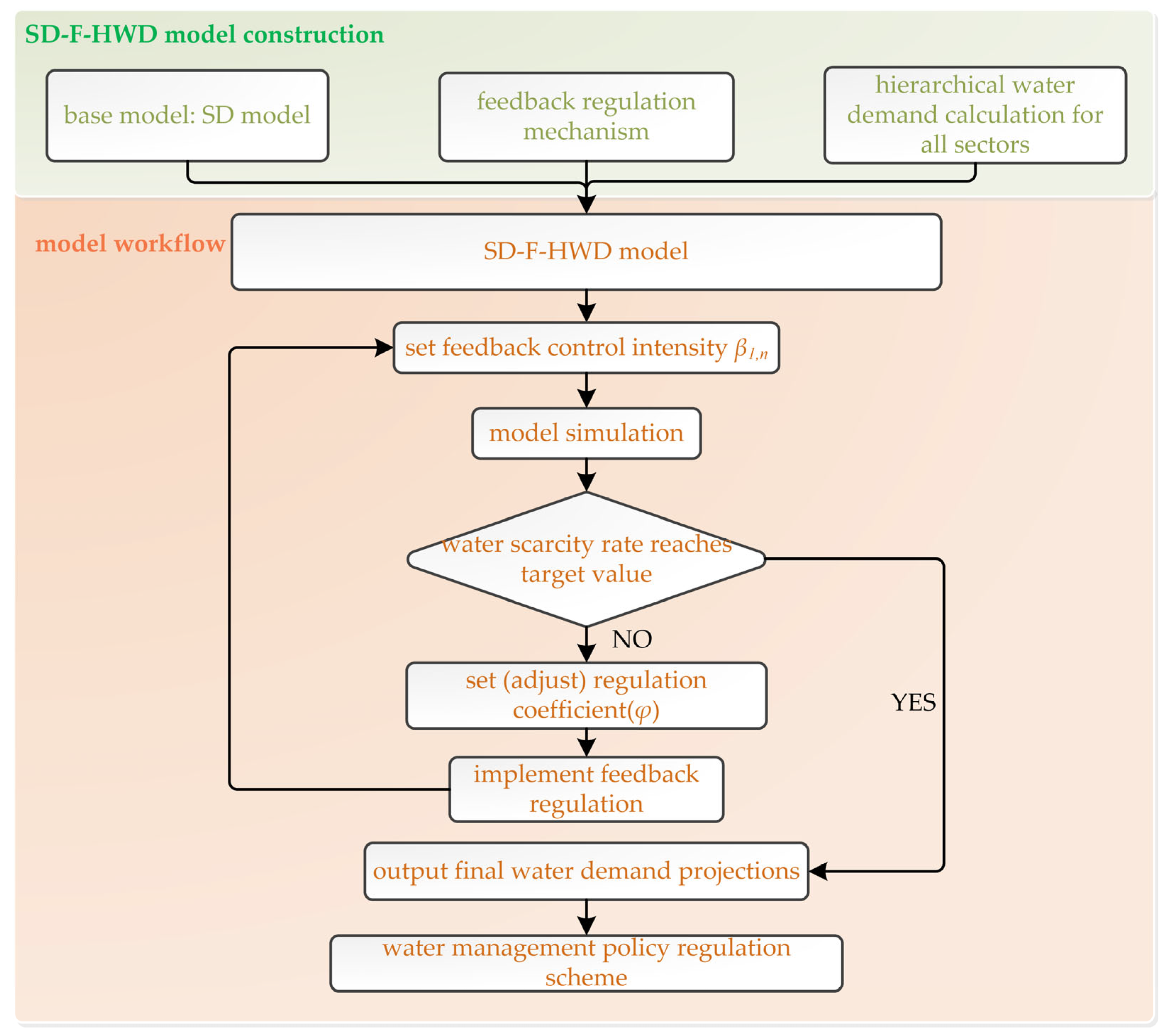
2.4. Workflow of the SD-F-HWD Model
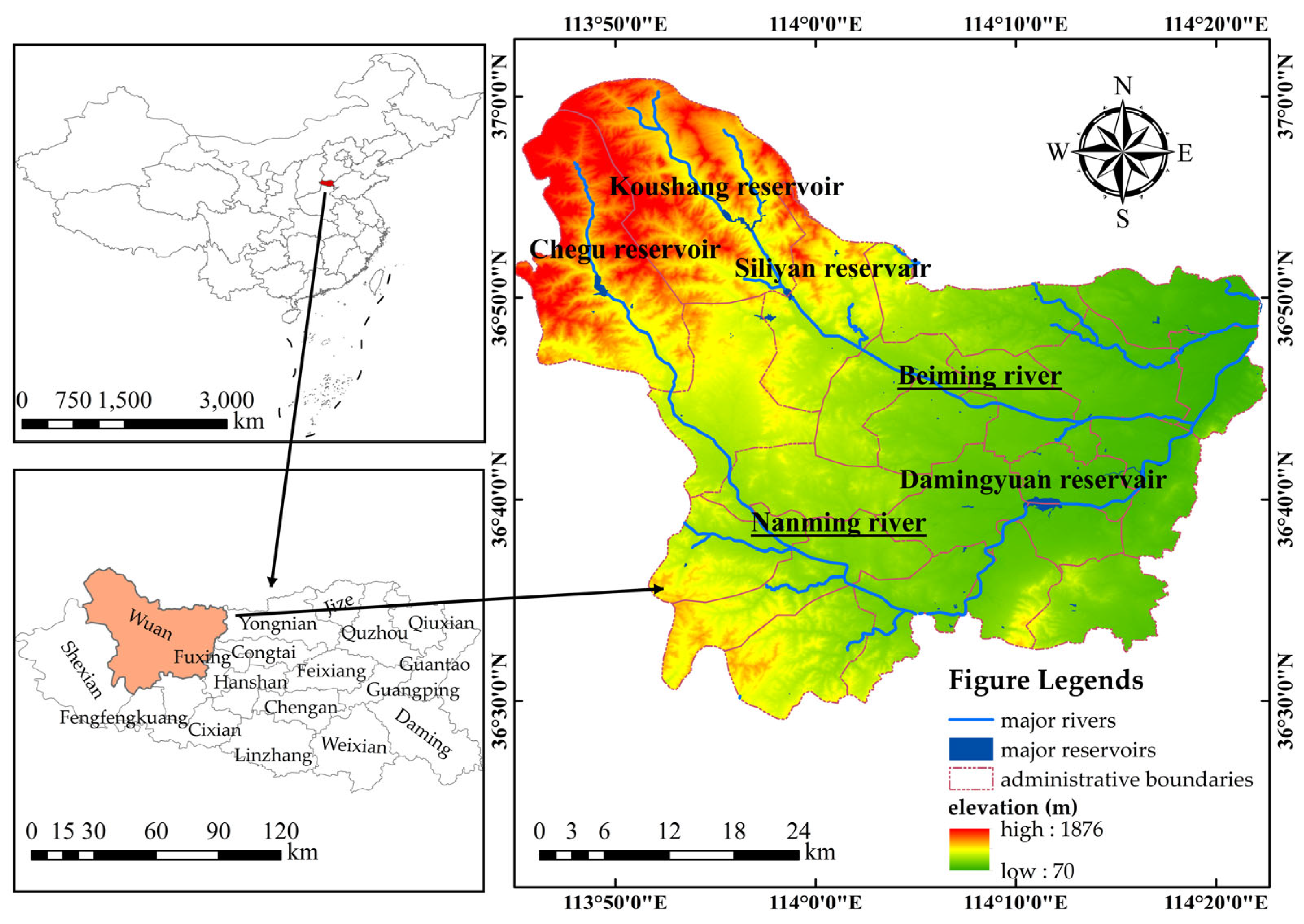
3. Case Study
3.1. Study Area
3.2. Data Resources
3.3. Application of the SD-F-HWD Model
3.3.1. Hierarchical Classification of Water Demand
3.3.2. Calculation of Water Supply
3.3.3. The SD-F-HWD Model of Wu’an City
3.4. Results
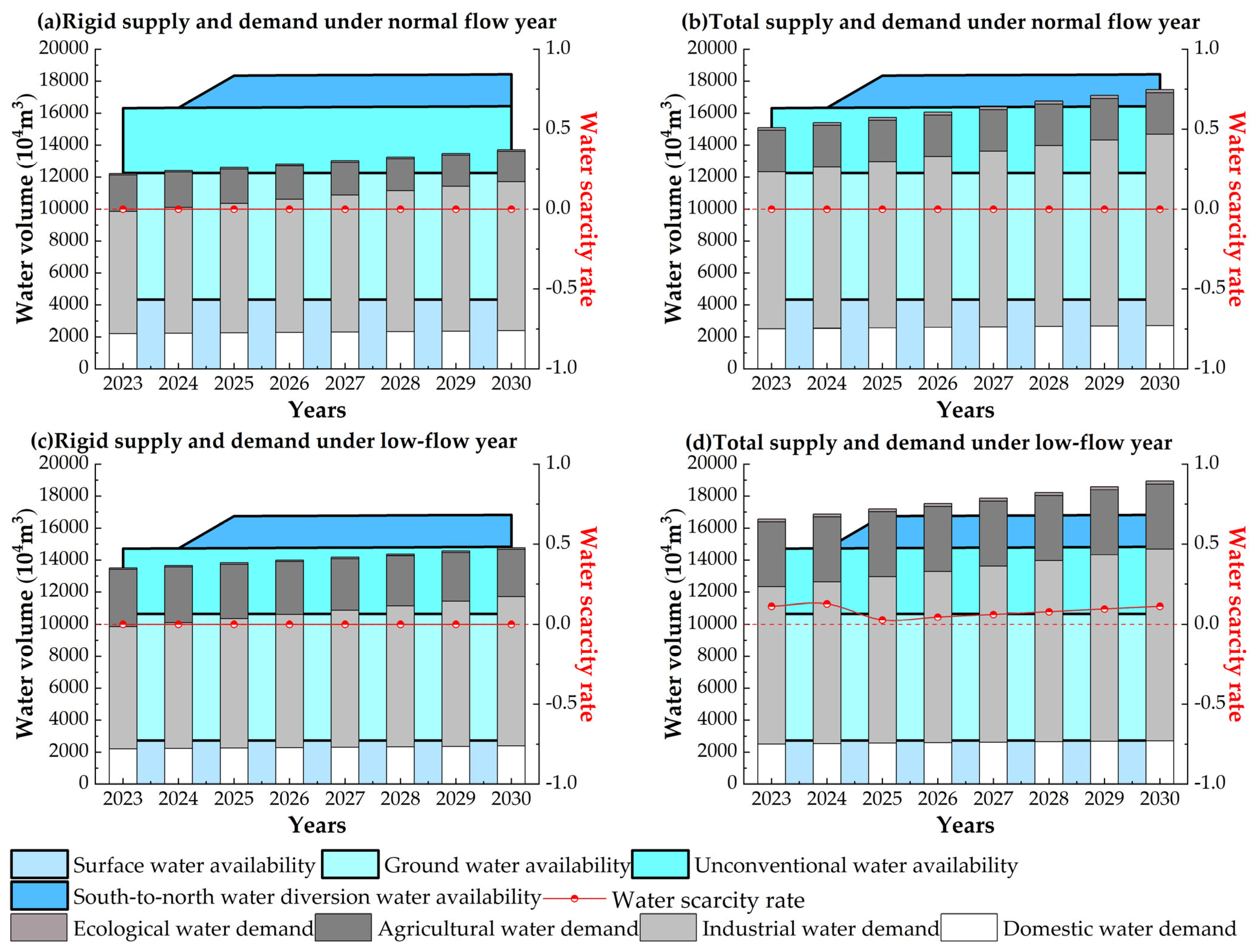
3.4.1. Water Supply and Demand Simulation
3.4.2. Feedback Regulation
4. Discussion
5. Conclusions
Supplementary Materials
Author Contributions
Funding
Data Availability Statement
Conflicts of Interest
References
- Salehi, M. Global Water Shortage and Potable Water Safety; Today’s Concern and Tomorrow’s Crisis. Environ. Int. 2022, 158, 106936. [Google Scholar] [CrossRef] [PubMed]
- Cheng, Y.; Fang, W.; Wu, Z. Research on Water Shortage Risks and Countermeasures in North China. AIP Conf. Proc. 2017, 1839, 020024. [Google Scholar] [CrossRef]
- Hao, R.; Huang, G.; Liu, L.; Li, Y.; Li, J.; Zhai, M. Sustainable Conjunctive Water Management Model for Alleviating Water Shortage. J. Environ. Manag. 2022, 304, 114243. [Google Scholar] [CrossRef] [PubMed]
- He, C.; Liu, Z.; Wu, J.; Pan, X.; Fang, Z.; Li, J.; Bryan, B.A. Future Global Urban Water Scarcity and Potential Solutions. Nat. Commun. 2021, 12, 4667. [Google Scholar] [CrossRef]
- Shemer, H.; Wald, S.; Semiat, R. Challenges and Solutions for Global Water Scarcity. Membranes 2023, 13, 612. [Google Scholar] [CrossRef]
- Ritchie, H.; Roser, M. Water Use and Stress; Our World in Data: Oxford, UK, 2024. [Google Scholar]
- Frini, A.; Benamor, S. Making Decisions in a Sustainable Development Context: A State-of-the-Art Survey and Proposal of a Multi-Period Single Synthesizing Criterion Approach. Comput. Econ. 2018, 52, 341–385. [Google Scholar] [CrossRef]
- Muzammil, M.; Zahid, A.; Farooq, U.; Saddique, N.; Breuer, L. Climate Change Adaptation Strategies for Sustainable Water Management in the Indus Basin of Pakistan. Sci. Total Environ. 2023, 878, 163143. [Google Scholar] [CrossRef]
- Ma, Z.; Liu, J.; Li, Y.; Zhang, H.; Fang, L. A BPNN-Based Ecologically Extended Input-Output Model for Virtual Water Metabolism Network Management of Kazakhstan. Environ. Sci. Pollut. Res. 2023, 30, 43752–43767. [Google Scholar] [CrossRef]
- Kassay, A.B.; Tuhar, A.W.; Ulsido, M.D. Integrated Modelling Techniques to Implication of Demographic Change and Urban Expansion Dynamics on Water Demand Management of Developing City in Lake Hawassa Watershed, Ethiopia. Environ. Res. Commun. 2023, 5, 055012. [Google Scholar] [CrossRef]
- Timotewos, M.T.; Barjenbruch, M.; Behailu, B.M. The Assessment of Climate Variables and Geographical Distribution on Residential Drinking Water Demand in Ethiopia. Water 2022, 14, 1722. [Google Scholar] [CrossRef]
- Vidal-Lamolla, P.; Molinos-Senante, M.; Oliva-Felipe, L.; Alvarez-Napagao, S.; Cortes, U.; Martinez-Gomariz, E.; Noriega, P.; Olsson, G.; Poch, M. Assessing Urban Water Demand-Side Management Policies before Their Implementation: An Agent-Based Model Approach. Sust. Cities Soc. 2024, 107, 105435. [Google Scholar] [CrossRef]
- Pei, D.; Wen, Y.; Li, W.; Ma, Z.; Guo, L.; Zhang, J.; Liu, M.; Mu, X.; Wang, Z. Agricultural Water Rebound Effect and Its Driving Factors in Xinjiang, China. Agric. Water Manag. 2024, 304, 109086. [Google Scholar] [CrossRef]
- Naderi, M.M.; Mirchi, A.; Bavani, A.R.M.; Goharian, E.; Madani, K. System Dynamics Simulation of Regional Water Supply and Demand Using a Food-Energy-Water Nexus Approach: Application to Qazvin Plain, Iran. J. Environ. Manag. 2021, 280, 111843. [Google Scholar] [CrossRef] [PubMed]
- Wang, B.; Tian, Y.; Li, X.; Li, C. Analysis and Prediction of Sustainable Utilization of Water Resources in Chengde City Based on System Dynamics Model. Water 2021, 13, 3534. [Google Scholar] [CrossRef]
- Dong, Q.; Zhang, X.; Chen, Y.; Fang, D. Dynamic Management of a Water Resources-Socioeconomic-Environmental System Based on Feedbacks Using System Dynamics. Water Resour. Manag. 2019, 33, 2093–2108. [Google Scholar] [CrossRef]
- Zhou, X.; Wang, F.; Huang, K.; Zhang, H.; Yu, J.; Alan, Y. Han System Dynamics-Multiple Objective Optimization Model for Water Resource Management: A Case Study in Jiaxing City, China. Water 2021, 13, 671. [Google Scholar] [CrossRef]
- White, P.A. Maslow’s Hierarchy of Needs and Water Management. J. Hydrol. 2020, 59, 1–16. [Google Scholar]
- Guo, D.; Zhang, D.; Xu, D.; Bian, Y.; Pan, Y. Multi-Objective Water Allocation for Wu’an City. Water 2025, 17, 153. [Google Scholar] [CrossRef]
- Wang, W.; Wang, T.; Liu, B.; Sha, J.; You, J. A Two-Stage Game-Based Model for Distribution of Water Consumption Control Indicators. J. Hydrol.-Reg. Stud. 2025, 58, 102259. [Google Scholar] [CrossRef]
- Naeem, K.; Zghibi, A.; Elomri, A.; Mazzoni, A.; Triki, C. A Literature Review on System Dynamics Modeling for Sustainable Management of Water Supply and Demand. Sustainability 2023, 15, 6826. [Google Scholar] [CrossRef]
- Qiao, J.; Shen, K.; Xiao, W.; Tang, J.; Chen, Y.; Xu, J. Integrating Graph Data Models in Advanced Water Resource Management: A New Paradigm for Complex Hydraulic Systems. Water 2025, 17, 3. [Google Scholar] [CrossRef]
- Rojas, M.; Méndez, A.; Watkins-Fassler, K. The Hierarchy of Needs Empirical Examination of Maslow’s Theory and Lessons for Development. World Dev. 2023, 165, 106185. [Google Scholar] [CrossRef]
- Wang, X.; Yu, M.; Sun, D.; Liu, G. Regional Water Demand Forecasting Based on Shared Socio-Economic Pathways in the Zhanghe River Basin. Water Policy 2023, 25, 908–926. [Google Scholar] [CrossRef]
- Li, Z.; Sun, F.; Liu, W.; Wang, T.; Wang, H.; Feng, Y. China’s Carbon Neutrality Policy Facilitates Halving Industrial Water Withdrawal. Environ. Res. Lett. 2024, 19, 114082. [Google Scholar] [CrossRef]
- Yadav, M.; Vashisht, B.B.; Jalota, S.K.; Jyolsna, T.; Singh, S.P.; Kumar, A.; Kumar, A.; Singh, G. Improving Water Efficiencies in Rural Agriculture for Sustainability of Water Resources: A Review. Water Resour. Manag. 2024, 38, 3505–3526. [Google Scholar] [CrossRef]
- Xiang, M.; Zhang, S.; Ruan, Q.; Tang, C.; Zhao, Y. Definition and Calculation of Hierarchical Ecological Water Requirement in Areas with Substantial Human Activity—A Case Study of the Beijing–Tianjin-Hebei Region. Ecol. Indic. 2022, 138, 108740. [Google Scholar] [CrossRef]
- Zhen, N.; Rutherfurd, I.; Webber, M. Ecological Water, a New Focus of China’s Water Management. Sci. Total Environ. 2023, 879, 163001. [Google Scholar] [CrossRef]
- Nikghalb, S.; Shokoohi, A.; Singh, V.P.; Yu, R. Ecological Regime versus Minimum Environmental Flow:Comparison of Results for a River in a Semi Mediterranean Region. Water Resour. Manag. 2016, 30, 4969–4984. [Google Scholar] [CrossRef]
- Xu, Q.; Song, W.; Zhang, Y. Forecast and Optimal Allocation of Production, Living and Ecology Water Consumption in Zhangye, China. Phys. Chem. Earth Parts A/B/C 2016, 96, 16–25. [Google Scholar] [CrossRef]
- Luo, Z.; Sun, Y.; Tang, G.; He, Z.; Peng, L.; Qi, D.; Ou, Z. The Relationship between Reference Crop Evapotranspiration Change Characteristics and Meteorological Factors in Typical Areas of the Middle of the Dry-Hot Valley of Jinsha River. Water 2024, 16, 1512. [Google Scholar] [CrossRef]
- Han, X.; Fu, M.; Wang, J.; Li, S. Optimizing Territorial Spatial Structures within the Framework of Carbon Neutrality: A Case Study of Wuan. Land 2024, 13, 1147. [Google Scholar] [CrossRef]
- Hou, B.; Yang, R.; Zhan, X.; Tian, W.; Li, B.; Xiao, W.; Wang, J.; Zhou, Y.; Zhao, Y. Conceptual Framework and Computational Research of Hierarchical Residential Household Water Demand. Water 2018, 10, 696. [Google Scholar] [CrossRef]
- Hou, B.D.; Yang, R.X.; Wang, J.H.; Xiao, W.H.; Zhao, Y.; Wang, H. Conceptual Framework of Hierarchical Water Demand. IOP Conf. Ser. Earth Environ. Sci. 2019, 344, 012074. [Google Scholar] [CrossRef]
- Timotewos, M.T.; Barjenbruch, M. Examining the Prospects of Residential Water Demand Management Policy Regulations in Ethiopia: Implications for Sustainable Water Resource Management. Sustainability 2024, 16, 5625. [Google Scholar] [CrossRef]
- Roberson, J.A. Lessons From 30 Years of Water Crises and Water Policy. J. Am. Water Work. Assoc. 2024, 116, 58–65. [Google Scholar] [CrossRef]
- Barone, S. The State against the Environment? Water Management and the Regulation of Tensions between Sectoral Policies in France. Environ. Policy Gov. 2025, 35, 3–12. [Google Scholar] [CrossRef]
- Sanchez, G.M.; Terando, A.; Smith, J.W.; García, A.M.; Wagner, C.R.; Meentemeyer, R.K. Forecasting Water Demand across a Rapidly Urbanizing Region. Sci. Total Environ. 2020, 730, 139050. [Google Scholar] [CrossRef]
- Mehrazar, A.; Massah Bavani, A.R.; Gohari, A.; Mashal, M.; Rahimikhoob, H. Adaptation of Water Resources System to Water Scarcity and Climate Change in the Suburb Area of Megacities. Water Resour. Manag. 2020, 34, 3855–3877. [Google Scholar] [CrossRef]
- Wang, X.; Zhang, J.; Shahid, S.; Guan, E.; Wu, Y.; Gao, J.; He, R. Adaptation to Climate Change Impacts on Water Demand. Mitig. Adapt. Strateg. Glob. Change 2016, 21, 81–99. [Google Scholar] [CrossRef]
- Nava, L.F.; Perera-Burgos, J.A. Key Challenges and Potential Opportunities in Water Management Crises: The Case of the Rio Turbio Basin in Mexico. Water 2025, 17, 550. [Google Scholar] [CrossRef]


| Variable | (%) | |
|---|---|---|
| total population | 0.24 | 0.999 |
| industrial value added | 3.04 | 0.738 |
| industrial water demand | 3.26 | 0.976 |
| domestic water demand | 0.50 | 0.778 |
| agricultural water demand | 1.18 | 0.654 |
| ecological water demand | 7.67 | 0.968 |
| total water demand | 2.17 | 0.902 |
| Adjustable Variables | Value | Upper Limit | Lower Limit | |
|---|---|---|---|---|
| water consumption per CNY 104 of industrial value added (m3/(CNY 104)) | 21.6 | / | 17.4 | |
| rural domestic water consumption quota (m3/(person·year)) | 22 | / | 18.5 | |
| urban domestic water consumption quota (m3/(person·year)) | 33.5 | / | 30 | |
| comprehensive irrigation water quota for forestry (m3/ha) | Normal-flow year | 2361.16 | / | 1863.12 |
| Low-flow year | 2593.71 | / | 2265.18 | |
| comprehensive irrigation quota for grain crops (m3/ha) | Normal-flow year | 1392.21 | / | 1167.17 |
| Low-flow year | 2229.76 | / | 1873.46 | |
| greening water quota (m3/(m2·a)) | 0.22 | / | / | |
| sewage treatment reuse rate (%) | 43.3 | 60 | / | |
| sewage collection coefficient (/) | 0.9 | 0.95 | / | |
| industrial value added growth rate (%) | 2.87 | / | 0.74 | |
| population growth rate (%) | 0.66 | / | 0 | |
| Scenario | Groups | 2030 Total Supply–Demand (Low-Flow Year) | |
|---|---|---|---|
| Feedback Control Intensity | Water Scarcity Rate (%) | ||
| S0 | / | 11.15 | |
| S1 | G1 | 0 | |
| S2 | G2 | 11.06 | |
| S3 | G3 | 9.45 | |
| S4 | G1,G2,G3 | 0 | |
| S5 | G1,G2,G3 | 9.64 | |
| S6 | G1,G2,G3 | 8.09 | |
| S7 | G1,G2,G3 | 6.49 | |
| S8 | G1,G2,G3 | 4.85 | |
| S9 | G1,G2,G3 | 3.21 | |
| S9 | G1,G2,G3 | 1.53 | |
| S11 | G1,G2,G3 | 0 | |
| S12 | G1,G2,G3 | 0 | |
| S13 | G1,G2,G3 | 0 | |
| Adjustable Variables | Before Feedback | After Feedback |
|---|---|---|
| per CNY 104 of industrial value added (m3/(CNY 104)) | 21.60 | 19.46 |
| rural domestic water consumption quota (m3/(person·year)) | 22.00 | 19.82 |
| urban domestic water consumption quota (m3/(person·year)) | 33.50 | 30.18 |
| comprehensive irrigation water quota for orchards on low-flow year (m3/ha) | 2593.71 | 2336.37 |
| comprehensive irrigation quota for grain crops on low-flow year (m3/ha) | 2229.76 | 2008.53 |
| greening water use quota (m3/(m2·year)) | 0.22 | 0.20 |
| industrial value added growth rate (/) | 0.43 | 0.48 |
| sewage collection coefficient (/) | 0.90 | 0.95 |
| industrial value added growth rate (%) | 2.87 | 2.58 |
| population growth rate (%) | 0.66 | 0.59 |
Disclaimer/Publisher’s Note: The statements, opinions and data contained in all publications are solely those of the individual author(s) and contributor(s) and not of MDPI and/or the editor(s). MDPI and/or the editor(s) disclaim responsibility for any injury to people or property resulting from any ideas, methods, instructions or products referred to in the content. |
© 2025 by the authors. Licensee MDPI, Basel, Switzerland. This article is an open access article distributed under the terms and conditions of the Creative Commons Attribution (CC BY) license (https://creativecommons.org/licenses/by/4.0/).
Share and Cite
Wang, R.; Zhang, S.; Sha, J.; Liu, B.; Zhang, D.; Wang, B. A Hierarchical Water Supply–Demand Regulation Model Coupling System Dynamics and Feedback Control Mechanisms: A Case Study in Wu’an City, China. Water 2025, 17, 1732. https://doi.org/10.3390/w17121732
Wang R, Zhang S, Sha J, Liu B, Zhang D, Wang B. A Hierarchical Water Supply–Demand Regulation Model Coupling System Dynamics and Feedback Control Mechanisms: A Case Study in Wu’an City, China. Water. 2025; 17(12):1732. https://doi.org/10.3390/w17121732
Chicago/Turabian StyleWang, Renlong, Shiwei Zhang, Jinxia Sha, Bin Liu, Dasheng Zhang, and Boxin Wang. 2025. "A Hierarchical Water Supply–Demand Regulation Model Coupling System Dynamics and Feedback Control Mechanisms: A Case Study in Wu’an City, China" Water 17, no. 12: 1732. https://doi.org/10.3390/w17121732
APA StyleWang, R., Zhang, S., Sha, J., Liu, B., Zhang, D., & Wang, B. (2025). A Hierarchical Water Supply–Demand Regulation Model Coupling System Dynamics and Feedback Control Mechanisms: A Case Study in Wu’an City, China. Water, 17(12), 1732. https://doi.org/10.3390/w17121732