

The Prediction of Aquifer Water Abundance in Coal Mines Using a Convolutional Neural Network–Bidirectional Long Short-Term Memory Model: A Case Study of the 1301E Working Face in the Yili No. 1 Coal Mine


Abstract
1. Introduction
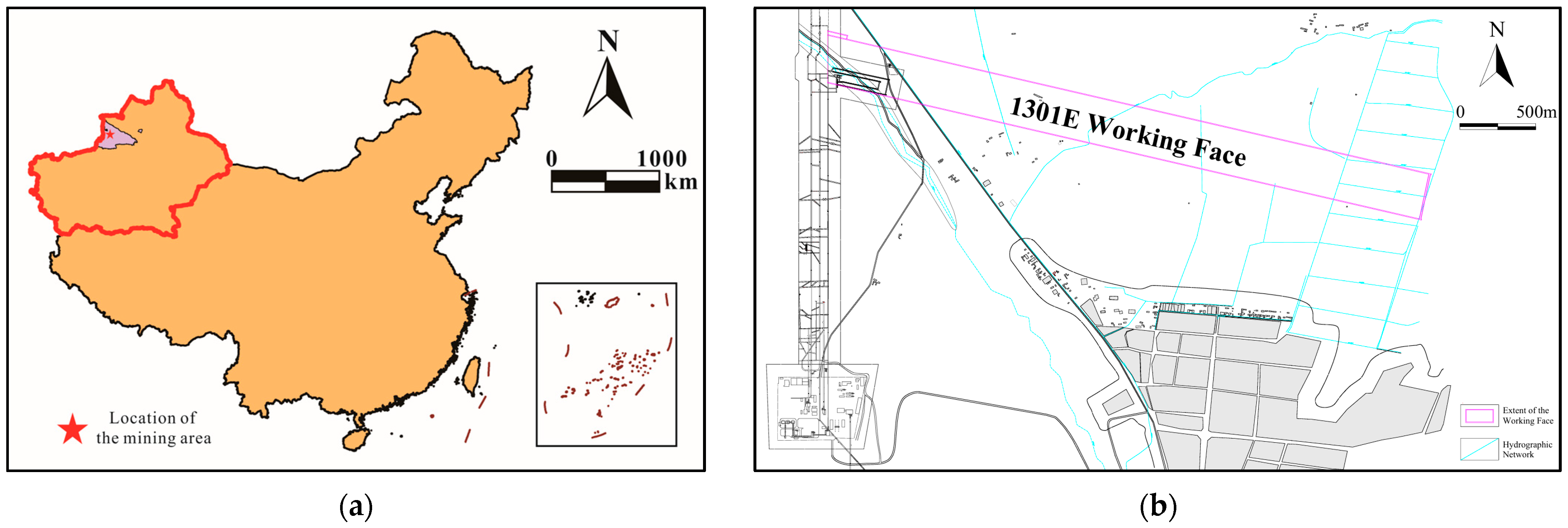
2. Study Area
3. Aquifer Water Abundance: Dominant Controlling Factors
3.1. Analysis of Dominant Controlling Factors of Water Abundance
- Aquifer depth:
- 2.
- Sand–mud ratio:
- 3.
- Hydraulic conductivity:
- 4.
- Core recovery:
- 5.
- Sand–mudstone interlayer number:
- 6.
- Equivalent Sandstone Thickness:
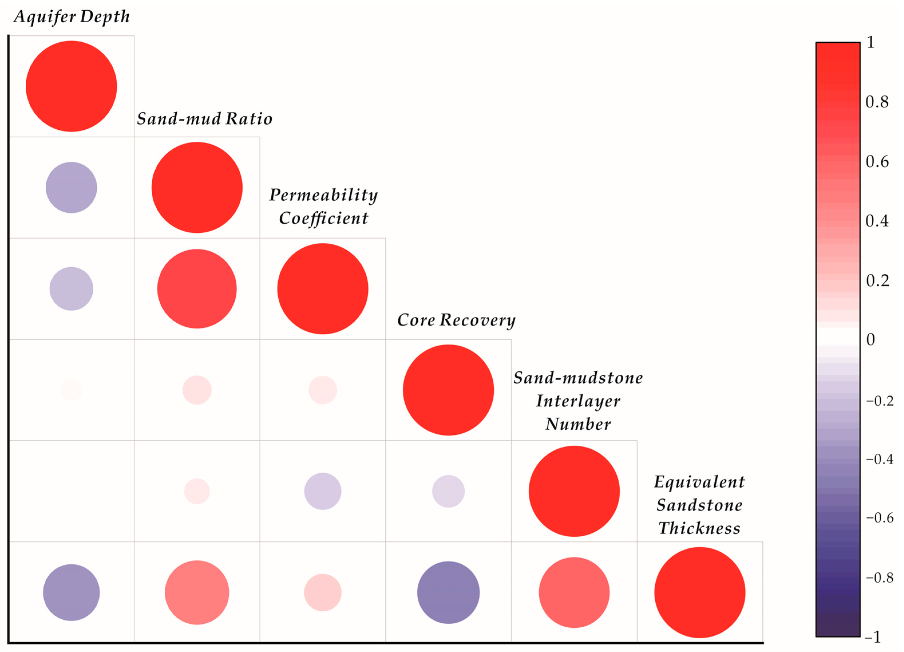
3.2. Correlation Analysis of Water Abundance Control Factors
4. Model Development and Application
4.1. CNN Convolutional Neural Network
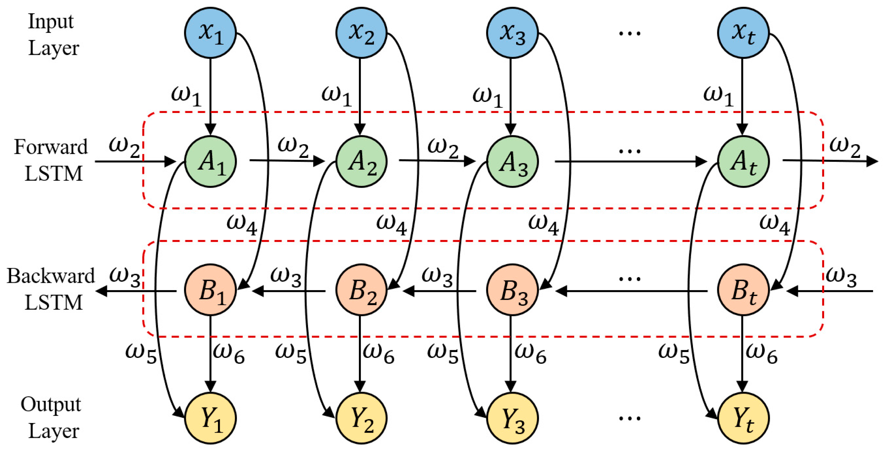
4.2. BiLSTM (Bidirectional Long Short-Term Memory) Network
4.3. CNN-BiLSTM Model
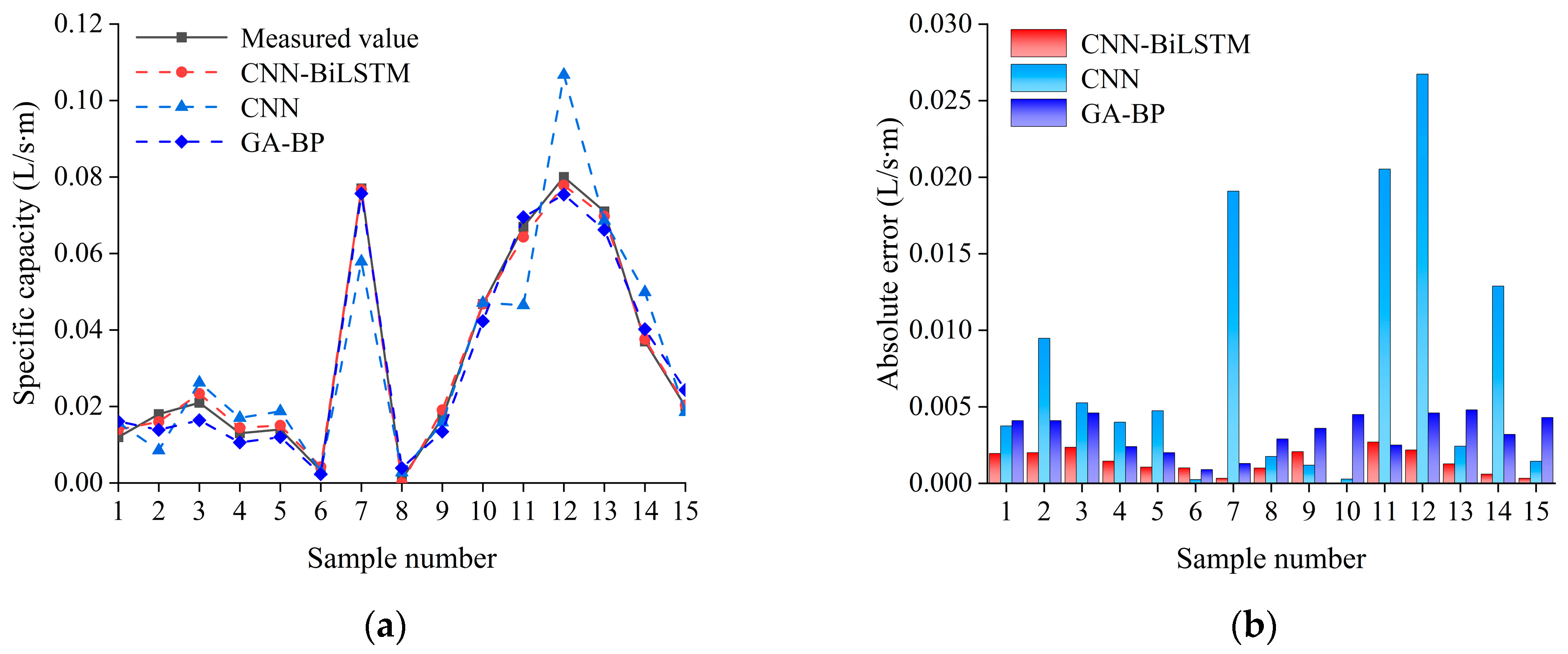
4.4. Case Analysis
5. Discussion
5.1. FAHP
5.2. Other Neural Network Prediction Models
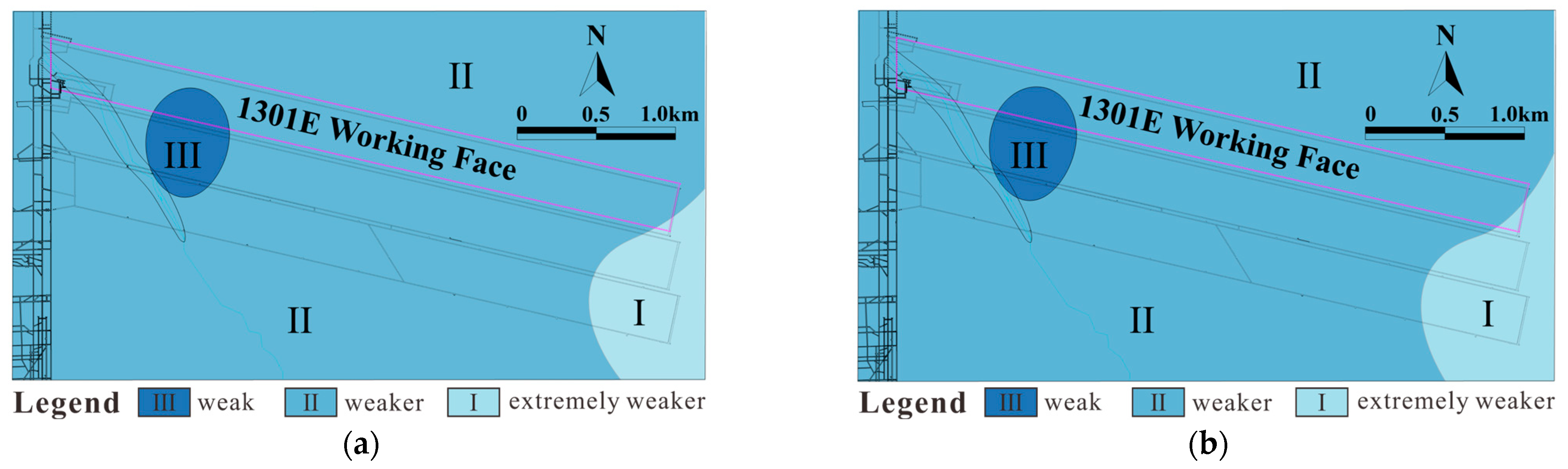
5.3. Productivity Zonation of Water Abundance
6. Conclusions
- (1)
- The five-category controlling factor system (including aquifer burial depth and hydraulic conductivity), screened via the kriging interpolation and Pearson correlation coefficients, effectively quantifies the regulatory effects of fracture development and lithologic combinations in weakly cemented strata on water abundance;
- (2)
- The CNN-BiLSTM model achieves collaborative modeling of localized spatial features and global nonlinear relationships through deep integration of convolutional kernels (32 channels) and BiLSTM hidden layers (64 units), attaining test set prediction accuracy (RMSE = 1.57 × 10⁻³, R2 = 0.9966) that improves by 85.2% over traditional FAHP methods, with 65.3% and 85.9% error reductions compared to the GA-BP and standalone CNN models, respectively;
- (3)
- The established three-tier water abundance zoning system (extremely weak/relatively weak/weak) achieves a 93.3% spatial consistency with field pumping test data, confirming the model’s engineering applicability under complex geological conditions.
Author Contributions
Funding
Data Availability Statement
Acknowledgments
Conflicts of Interest
References
- Sun, W.J.; Li, W.J.; Ning, D.Y. Current situation, prediction and prevention suggestions of coal mine water disaster accidents in China. Coal Geol. Explor. 2023, 51, 185–194. [Google Scholar]
- Wu, Q.; Guo, X.M.; Bian, K. Conducting a census of water disaster risk factors to prevent coal mine water disaster accidents. Chin. Coal. 2023, 49, 3–15. [Google Scholar]
- Jiang, Z.L.; Tian, Y.H. Integrated geophysical technology applied to watery evaluation of sinkhole. Coal Sci. Technol. 2015, 43, 139–142. [Google Scholar]
- Li, M.X. Exquisite exploration of Jurassic burnt rock water abundance of northern part of Tarim Basin. Coal Min. Technol. 2018, 23, 15–17. [Google Scholar]
- Yang, B.B.; Yuan, J.H.; Duan, L.H. Development of a system to assess vulnerability of flooding from water in karst aquifers induced by mining. Environ. Earth Sci. 2018, 77, 91. [Google Scholar] [CrossRef]
- Zeng, Y.F.; Wu, Q.; Liu, S.Q. Evaluation of a coal seam roof water inrush: Case study in the Wangjialing coal mine. China Mine Water Environ. 2018, 37, 174–184. [Google Scholar] [CrossRef]
- Shen, J.J.; Wu, Q.; Liu, W.T. The development of the water-richness evaluation model for the unconsolidated aquifers based on the extension matter-element theory. Geotech. Geol. Eng. 2020, 38, 2639–2652. [Google Scholar] [CrossRef]
- Lyu, Z.M.; Meng, F.Z.; Lyu, W.M.; Li, L.N. Improved Method for Predicting and Evaluating Water Yield Property. Coal Technol. 2023, 42, 152–155. [Google Scholar]
- Qiu, Z.L.; Chen, W.H.; Bao, D.L.; Liu, Y.H.; Feng, J.W.; Huang, C.M. Combined Detection of Mine Water Disasters with Various Geophysical Prospecting Techniques. Min. Saf. Environ. Prot. 2016, 43, 60–63. [Google Scholar]
- Wu, Q. Progress, problems and prospects of prevention and control technology of mine water and reutilization in China. J. China Coal Soc. 2014, 39, 795–805. [Google Scholar]
- Wu, Q.; Wang, Y.; Zhao, D.K.; Shen, J.J. Water abundance assessment method and application of loose aquifer based on sedimentary characteristics. J. China Univ. Min. Technol. 2017, 46, 460–466. [Google Scholar]
- Zheng, Q.S.; Wang, C.F. Research on optimization model and algorithm for mine water inrush risk prediction based on multivariate ensemble analysis. Chin. J. Manag. Sci. 2023, 1, 41. [Google Scholar]
- Li, L.N.; Wei, J.C.; Li, L.Y.; Shi, S.Q.; Yin, H.Y. Water yield property prediction model of aquifer based on logging data: A case study from Yingpanhao mine field in Ordos area. China Min. Mag. 2019, 28, 143–147. [Google Scholar]
- Wu, Q.; Xu, K.; Zhang, W. Further discussion on the “Three-map-double prediction method” for predicting and evaluating the risk of water inrush from coal seam roof. J. Coal. 2016, 41, 1341–1347. [Google Scholar]
- Wu, Q.; Fan, Z.L.; Liu, S.Q.; Zhang, Y.W.; Sun, W.J. Evaluation method of water abundance of information fusion aquifer based on GIS-water abundance index method. J. Coal. 2011, 36, 1124–1128. [Google Scholar]
- Wu, Q.; Wang, J.H.; Liu, D.H.; Cui, F.P.; Liu, S.Q. A new practical method for evaluating water inrush from coal seam floor IV: Application of AHP vulnerability index method based on GIS. J. Coal. 2009, 34, 233–238. [Google Scholar]
- Xue, J.K.; Shi, L.; Wang, H.; Ji, Z.K.; Shang, H.B.; Xu, F.; Zhao, C.H. Water abundance evaluation of a burnt rock aquifer using the AHP and entropy weight method: A case study in the Yongxin coal mine, China. Mine Water Erviron. 2021, 80, 417. [Google Scholar] [CrossRef]
- Li, L.N.; Li, W.P.; Shi, S.Q.; Yang, Z.; He, J.H.; Chen, W.C.; Yang, Y.R.; Zhu, T.E.; Wang, Q.Q. An Improved Potential Groundwater Yield Zonation Method for Sandstone Aquifers and Its Application in Ningxia, China. Nat. Res. Res. 2022, 31, 849–865. [Google Scholar] [CrossRef]
- Li, Q.F.; Cui, H.; Xiao, L.L.; Liu, K.; Xu, X. Water abundance and water inrush risk assessment of Jurassic coal seam roof in Ningzheng Coalfield. J. Xi’an Univ. Sci. Technol. 2023, 43, 523–529. [Google Scholar]
- Han, C.; Pan, X.H.; Li, G.L.; Tu, J.N. Fuzzy Analytic hierarchy process of aquifer Water abundance based on GIS Multi-source Information Integration. Hydrogeol. Eng. Geol. 2012, 39, 19–25. [Google Scholar]
- Xue, S.; Li, W.P.; Guo, Q.C.; Liu, S.L.; Sun, M.Y.; Fan, B.J. Prediction of water abundance of roof confined aquifer based on FAHP-GRA evaluation method. Metal. Mine 2018, 4, 168–172. [Google Scholar]
- Li, Z.; Zeng, Y.F.; Liu, S.Q.; Gong, H.J.; Niu, P.K. Application of BP artificial neural network in water abundance evaluation. Coal Eng. 2018, 50, 114–118. [Google Scholar]
- Gong, H.J.; Zeng, Y.F.; Liu, S.Q.; Li, Z.; Niu, P.K. Evaluation of aquifer abundance based on improved fuzzy analytic hierarchy process. Coal Technol. 2018, 37, 158–159. [Google Scholar]
- Chen, J.P.; Wang, C.L.; Wang, X.D. Prediction of water inrush from coal seam floor based on CNN neural network. Chin. J. Geol. Hazard Control 2021, 32, 50–57. [Google Scholar]
- Yin, H.Y.; Shi, Y.L.; Niu, H.G.; Xie, D.L.; Wei, J.C.; Liliana, L.; Xu, S.X. A GIS-based model of potential groundwater yield zonation for a sandstone aquifer in the Juye Coalfield, Shangdong, China. J. Hydrol. 2018, 557, 434–447. [Google Scholar] [CrossRef]
- Yang, F.; Feng, X.; Ruan, L.; Chen, J.W.; Xia, R.; Chen, Y.L.; Jin, Z.H. Study on the correlation between water branches and ultra-low frequency dielectric loss based on Pearson correlation coefficient method. High Volt. Electr. Appl. 2014, 50, 21–25, 31. [Google Scholar]
- Dong, L.P.; Nie, Q.H.; Sun, X.K. Analysis of the influence of shield tunneling parameters on ground surface settlement based on Pearson correlation coefficient method. Constr. Technol. 2024, 53, 116–123. [Google Scholar]
- Ding, Y.J.; Wang, Z.C.; Xin, Y.; Liu, W.L.; Cheng, M. Structural nonlinear model updating based on CNN-BiLSTM-Attention hybrid neural network. Eng. Mech. 2025, 1, 1–13. [Google Scholar]
- Zhang, X.J.; Wang, C.; Zhang, J.H. Integrated energy system load forecasting based on multi-energy demand response and improved BiLSTM. Electr. Power Constr. 2025, 46, 113–125. [Google Scholar]
- Méndez, M.; Merayo, M.G.; Núñez, M. Long-term traffic flow forecasting using a hybrid CNN-BiLSTM model. Eng. Appl. Artif. Intell. 2023, 121, 106041. [Google Scholar] [CrossRef]
- Xie, H.X.; Zhang, X.; Dong, J.Y. Prediction model of mine gas emission based on CNN-BiLSTM. China J. Saf. Sci. Technol. 2024, 20, 53–59. [Google Scholar]
- Wang, L.; Xiong, J.Y.; Ruan, C.L. Research on product design of FAHP bone marrow aspiration needle. Heliyon. 2024, 10, e27389. [Google Scholar] [CrossRef]
- National Mine Safety Administration. Coal Mine Water Prevention and Control Rules; China Coal Industry Publishing House: Beijing, China, 2008. [Google Scholar]


| Dominant Controlling Factors | Aquifer Depth | Sand–Mud Ratio | Hydraulic Conductivity | Core Recovery | Sand–Mudstone Interlayer Number | Equivalent Sandstone Thickness |
|---|---|---|---|---|---|---|
| 95% confidence interval coverage rate | 93.3% | 100% | 93.3% | 93.3% | 100% | 93.3% |
| Sample Number | Actual Value L/(s·m) | Water Abundance Class | Predicted Value L/(s·m) | Water Abundance Class | Error |
|---|---|---|---|---|---|
| 1 | 0.012 | Weak | 0.058 | Weak | 0.046 |
| 2 | 0.018 | Weak | 0.042 | Weak | 0.024 |
| 3 | 0.021 | Weak | 0.047 | Weak | 0.026 |
| 4 | 0.013 | Weak | 0.056 | Weak | 0.043 |
| 5 | 0.014 | Weak | 0.056 | Weak | 0.042 |
| 6 | 0.003 | Weak | 0.024 | Weak | 0.021 |
| 7 | 0.077 | Weak | 0.064 | Weak | −0.013 |
| 8 | 0.001 | Weak | 0.072 | Weak | 0.071 |
| 9 | 0.017 | Weak | 0.064 | Weak | 0.047 |
| 10 | 0.047 | Weak | 0.117 | Medium | 0.070 |
| 11 | 0.067 | Weak | 0.063 | Weak | −0.004 |
| 12 | 0.080 | Weak | 0.122 | Medium | 0.042 |
| 13 | 0.071 | Weak | 0.065 | Weak | −0.006 |
| 14 | 0.037 | Weak | 0.083 | Weak | 0.046 |
| 15 | 0.020 | Weak | 0.066 | Weak | 0.046 |
| Sample Number | Actual Value | GA-BP | GA-BP Absolute Errors | CNN | CNN Absolute Errors | CNN-BiLSTM | CNN-BiLSTM Absolute Errors |
|---|---|---|---|---|---|---|---|
| 1 | 0.012 | 0.016 | 0.0041 | 0.016 | 0.0038 | 0.014 | 0.046 |
| 2 | 0.018 | 0.014 | 0.0041 | 0.009 | 0.0095 | 0.016 | 0.024 |
| 3 | 0.021 | 0.016 | 0.0046 | 0.026 | 0.0053 | 0.023 | 0.026 |
| 4 | 0.013 | 0.011 | 0.0024 | 0.017 | 0.0040 | 0.014 | 0.043 |
| 5 | 0.014 | 0.012 | 0.0020 | 0.019 | 0.0047 | 0.015 | 0.042 |
| 6 | 0.003 | 0.002 | 0.0009 | 0.003 | 0.0002 | 0.004 | 0.021 |
| 7 | 0.077 | 0.076 | 0.0013 | 0.058 | 0.0191 | 0.077 | −0.013 |
| 8 | 0.001 | 0.004 | 0.0029 | 0.003 | 0.0018 | 0.000 | 0.071 |
| 9 | 0.017 | 0.013 | 0.0036 | 0.016 | 0.0012 | 0.019 | 0.047 |
| 10 | 0.047 | 0.042 | 0.0045 | 0.047 | 0.0003 | 0.047 | 0.070 |
| 11 | 0.067 | 0.070 | 0.0025 | 0.046 | 0.0205 | 0.064 | −0.004 |
| 12 | 0.080 | 0.075 | 0.0046 | 0.107 | 0.0267 | 0.078 | 0.042 |
| 13 | 0.071 | 0.066 | 0.0048 | 0.069 | 0.0024 | 0.070 | −0.006 |
| 14 | 0.037 | 0.040 | 0.0032 | 0.050 | 0.0129 | 0.038 | 0.046 |
| 15 | 0.020 | 0.024 | 0.0043 | 0.019 | 0.0014 | 0.020 | 0.046 |
Disclaimer/Publisher’s Note: The statements, opinions and data contained in all publications are solely those of the individual author(s) and contributor(s) and not of MDPI and/or the editor(s). MDPI and/or the editor(s) disclaim responsibility for any injury to people or property resulting from any ideas, methods, instructions or products referred to in the content. |
© 2025 by the authors. Licensee MDPI, Basel, Switzerland. This article is an open access article distributed under the terms and conditions of the Creative Commons Attribution (CC BY) license (https://creativecommons.org/licenses/by/4.0/).
Share and Cite
Ye, Y.; Li, W.; Yang, Z.; Li, X.; Wang, Q. The Prediction of Aquifer Water Abundance in Coal Mines Using a Convolutional Neural Network–Bidirectional Long Short-Term Memory Model: A Case Study of the 1301E Working Face in the Yili No. 1 Coal Mine. Water 2025, 17, 1595. https://doi.org/10.3390/w17111595
Ye Y, Li W, Yang Z, Li X, Wang Q. The Prediction of Aquifer Water Abundance in Coal Mines Using a Convolutional Neural Network–Bidirectional Long Short-Term Memory Model: A Case Study of the 1301E Working Face in the Yili No. 1 Coal Mine. Water. 2025; 17(11):1595. https://doi.org/10.3390/w17111595
Chicago/Turabian StyleYe, Yangmin, Wenping Li, Zhi Yang, Xiaoqin Li, and Qiqing Wang. 2025. "The Prediction of Aquifer Water Abundance in Coal Mines Using a Convolutional Neural Network–Bidirectional Long Short-Term Memory Model: A Case Study of the 1301E Working Face in the Yili No. 1 Coal Mine" Water 17, no. 11: 1595. https://doi.org/10.3390/w17111595
APA StyleYe, Y., Li, W., Yang, Z., Li, X., & Wang, Q. (2025). The Prediction of Aquifer Water Abundance in Coal Mines Using a Convolutional Neural Network–Bidirectional Long Short-Term Memory Model: A Case Study of the 1301E Working Face in the Yili No. 1 Coal Mine. Water, 17(11), 1595. https://doi.org/10.3390/w17111595