1. Introduction
Underwater natural gas pipelines (UNGPs) are used to collect and transport natural gas underwater. The safety and reliability of UNGPs are crucial to preventing natural gas waste and protecting the natural environment and underwater life [
1]. However, due to the complex environment and poor underwater conditions, UNGPs are at great risk of damage and leaks, which could result in enormous hazards and safety issues. Therefore, the inverse identification of UNGP leakage sources is of great significance to identifying dangerous situations, enabling a fast response, and ensuring safe and reliable underwater pipeline operation.
Based on previous studies, it can be inferred that leakage and dispersion estimations for UNGPs have attracted significant interest, mainly in relation to the process by which the leaked gas diffuses in the water [
2,
3]. Focusing on this topic, there are various research methods for detecting and positioning leakages, such as those using semi-conductors, optical cameras, biosensors, fiber optic cables, and acoustics [
4]. Among these technologies, underwater optical images are frequently investigated because they offer high resolution and rich information and are easy to analyze via depth learning theory.
The gas leaked from a damaged UNGP port carries water upward to form bubble plumes. Bubble plumes are inevitable, have a long life, and are difficult to model [
5]. Due to the influence of turbulence and pipe pressure, the bubble density, compressibility, and other parameters of the plumes are obviously different from the parameters of these bubbles in water and other types of underwater bubbles. Therefore, instantaneous optical underwater bubble plume images can provide rich information on the spatial structure and flow characteristics of the flow field [
6].
Under the influence of the complex underwater environment, the density and compressibility of the bubbles change significantly from the site of the damaged port to the surface. With the rapid development of image-processing technology, it is possible to accurately identify underwater bubble plumes and extract the morphological characteristics of their diffusion movement. Therefore, instantaneous optical images can provide rich information about UNGP leakage sources. However, it is very difficult to obtain sufficient multi-scale features from underwater bubble plume images because of their chaotic backgrounds and complex environment. Our research team has developed new methods of obtaining multi-scale morphological features from underwater bubble plume images, and these methods have achieved good convergence speed and recognition accuracy for underwater bubble plumes [
7]. Some research has already been conducted in this area. The ascending motion of the bubble plumes contains a wealth of information about the diffusion of underwater bubbles [
8], which can provide a solid basis for leak traceability. This study uses computational fluid dynamics techniques to simulate the diffusion pattern of natural gas leaking from a pipeline [
9], and the process of bubble plume diffusion in water can be simulated more accurately using computational fluid modeling [
10,
11].
A geometric model of underwater gas diffusion can be used to quantitatively determine the full-cycle scale distribution law of the motion of bubble plumes from the leakage outlet to the water surface. Key traceability parameters can be obtained via dimension analysis, which can provide accurate positioning clues for tracing a pipeline gas leakage in the flow field environment. Some research has also been conducted on underwater bubble plumes [
12,
13,
14].
At present, most underwater traceability research focuses on the identification of groundwater pollution sources. Many of these findings are also helpful regarding underwater bubble plume traceability. A groundwater pollution source identification method combining the advection–dispersion equation (ADE) for contaminants in groundwater with a genetic algorithm (GA) was proposed in [
15], and the backward probability method was utilized to identify a river in [
16]. Intelligent methods were also used to trace groundwater pollutants in [
17,
18], significantly improving the traceability accuracy.
However, to the best of our knowledge, there is currently no approach to the inverse identification of UNGP leakage sources based on underwater bubble plume optical images, particularly with respect to the underwater diffusion law of bubble plumes. Hence, a UNGP leakage source inverse identification method based on optical underwater images, which are easy to obtain, is urgently needed. Similar to the inversion identification of groundwater pollution, tracing UNGP bubble plumes is also an inverse mathematical problem, and the simulation–optimization method is widely used in solving underwater traceability inversion problems. A number of model-based convolutional neural network (CNN) approaches are presented as alternative methods to optimize the inverse identification model [
19]. According to previous research [
20], the alternative simulation models established via the Kriging and neural network methods achieve high fitting accuracy and can be used to solve inverse identification problems. On the other hand, the Kalman filter is an optimal state estimation method, which can be applied to dynamic systems with random interference. Previous studies have reported that the Kalman filter is also an effective method for determining underwater traceability [
21,
22].
In conclusion, traditional detection methods based on the damage itself have limitations in terms of time and space, and taking only the underwater bubble as the detection target does not eliminate the influence of the underwater wave field environment on the bubble’s morphology. Therefore, taking the underwater bubble plume as the detection target; making use of its wide distribution range and long survival time; and fully integrating and understanding image features, wave field environment, and other multi-source information to improve the accuracy of bubble plume identification and traceability can effectively promote the development of submarine pipeline leakage traceability technology and provide a stable and effective method for the comprehensive identification of UNGP leakages.
In this study, based on the framework of the simulation–optimization method, a joint identification approach to tracing UNGP bubble plumes and determining model parameters is proposed. Essentially, there are two sub-models in the simulation–optimization method, namely, a numerical model and a surrogate model. First, a numerical model of underwater bubble plume diffusion is constructed, and a hypothetical example is constructed with the forward prediction results to verify the effectiveness of the method. Then, in order to reduce the computational load in the inversion process, the surrogate model is constructed to optimize the numerical model. Finally, the optimized surrogate model is solved using the simulated annealing method, and the identification results are obtained.
2. Methodology
2.1. Underwater Bubble Plume Research
Bubbles from a UNGP leak can be used as a basis for finding the leak source. At present, leakage source detection technologies based on underwater optical images often consider the breach the research object and inspect the pipeline when investigating and tracing the leakage source. Due to the complex and time-varying nature of the underwater environment, this inspection approach is time-consuming, and the ability to observe time and space conditions is limited. Furthermore, the morphology of broken pipeline ports is random and diversified, which makes it difficult to describe and characterize the target features in a unified way.
Conventional ideas and techniques are no longer sufficient to overcome the challenges encountered by underwater tracing technologies. The gas leaking from a pipeline breach, entrapped in seawater, moves upward to form bubble plumes, and instantaneous optical images of these plumes contain rich information about the spatial structure of the wave field and flow characteristics. Based on a geometric model of underwater gas diffusion, a full-cycle scale distribution law for the movement of bubble plumes from the leakage port to the water surface can be quantified. From this law, the key parameters of traceability can be obtained via downscaling analysis, which can provide accurate localization clues for tracing a pipeline gas leak in a wave field environment.
2.2. Simulation-Optimization Method
At present, simulation–optimization methods are widely used for solving groundwater pollution inversion problems. When a simulation–optimization method is combined with the binary genetic algorithm, the hydrogeological parameters can be solved more accurately [
23]. Simulation–optimization methods based on artificial neural networks can also successfully identify pollution sources in water [
24]. However, it remains difficult to identify pollution sources using traditional simulation–optimization methods when both the pollution source and model parameters are unknown.
Tracing bubble plumes from UNGPs is very similar to the principle of tracing underwater contaminants; both require the inverse solution of underwater dispersion values using limited and discrete dynamic observation data. From the perspective of operations research, the problem of the inversion of UNGP leakage traceability and model parameters can be transformed into an optimization problem that takes the leakage source and model parameters as the variables to be solved, the monitoring value of the bubble plume morphology parameters as close as possible to the simulated calculated values as the optimization objective, and the underwater bubble diffusion model as the constraint to form a minimization problem with constraints.
The simulation–optimization method is divided into two parts: building a simulation model and building an optimization model. For the simulation model, since a basic model of the bubble plume was established and perfected and following the vigorous development of computerized fluid dynamics (CFD) simulation technology, scholars have quantitatively estimated the parameters of the motion pattern of bubble plumes in a wave field environment based on the volume of fluid (VOF) model [
25,
26]. A numerical model of underwater gas pipeline leak diffusion was gradually established by analyzing the variation of the key parameters of the bubble plume formed in the wave field when a leak occurred in an underwater gas transmission pipeline [
27,
28]. Based on the underwater gas diffusion geometry model, the motion of the underwater bubble plume can be effectively simulated, providing a suitable numerical simulation for the optimization of the UNGP leak traceability simulation.
Heuristic algorithms are mostly used to solve optimization models. Commonly used heuristic algorithms include genetic algorithms and the simulated annealing method. The simulated annealing method selects the optimal solution interval via random model perturbation, constantly updates the state model, and iterates until the optimal solution is obtained. Since the simulated annealing method demonstrates faster convergence and is less likely to fall into a local optimal solution [
29], it was chosen for solving the optimization model in this study.
In order to invert the UNGP leakage source, an underwater bubble plume diffusion simulation–optimization approach is proposed. A simulation model of underwater bubble plume diffusion is built so as to establish an input–output response system to simulate the spatial and temporal distribution characteristics of the bubble plumes from the leak point to the water surface. During optimization, the sum of the squares of the differences between the simulated calculated values and the actual observed bubble plume diffusion parameter values is used as the objective function.
To solve this model, bubble diffusion velocity and bubble radius models are coupled to the optimization model. By continuously invoking the simulation–optimization method, the results of each simulation are compared with the actual observed data until the difference between the two is minimal, thus achieving the continuous optimization of the model parameters and finally obtaining a solution that provides simulation results as close as possible to the observed data.
2.3. Underwater Bubble Plume Diffusion Numerical Model
Based on the established coupled model of bubble motion in the wave field, the interaction law of the influencing factors in the upwelling motion of bubbles in the wave field can be characterized more accurately [
30]. The coupled model of bubble upwelling motion in the wave field can be obtained by combining the mass transfer differential equation, bubble heat transfer differential equation, velocity differential equation, and radius differential equation. Since it is very difficult to accurately determine the bubble mass and inner temperature from images of underwater bubble plumes, in this study, according to the bubble plume identification results, the bubble diffusion velocity model and the bubble radius model are established to simulate the bubble plume motion in the wave field.
A bubble velocity point set is obtained based on the results of the analysis of the bubble particle characteristics in the bubble plumes. The bubble particle velocity profile is obtained by filtering according to the number of point sets, and the abnormal point sets with small numbers are removed [
31]. Finally, a velocity differential equation is obtained by fitting based on the underwater bubble diffusion velocity model, which can be defined as follows:
where
is the bubble particle velocity,
is the wave velocity,
is the average bubble radius,
is a constant,
is the generalized pressure in the breaking wave field,
is the fluid velocity field, and
.
In the same way, a bubble radius point set is obtained based on the analysis of the bubble particle characteristics in the bubble plumes. The bubble particle radius curve is obtained by filtering out unreasonably large or small radius data. Finally, the radius differential equation is fitted based on the bubble radius model, which is defined as follows:
where
represents the bubble density,
represents the ratio of the universal gas constant to the molar mass of the gas,
represents the water temperature,
represents the liquid surface tension coefficient,
represents the generalized pressure in the breaking wave field,
represents the bubble radius, and
.
2.4. Surrogate Models
The simulation–optimization method is used to solve the inverse identification problem of underwater traceability, which requires multiple invocations of the numerical simulation model for the bubble plumes’ underwater diffusion and generates a large computational load. Therefore, it is necessary to introduce surrogate models to improve the computational efficiency and reduce the computational load. The surrogate model construction methods that have been applied in the field of underwater traceability research are artificial neural networks (ANNs), radial basis function methods, and the Kriging method [
32]. According to previous studies, both the Kriging and neural network methods achieve a high fitting accuracy, which is suitable for the underwater bubble plume retrospective inversion carried out in this study.
The trained surrogate model can obtain the input–output response relationship, which is similar to the relationship of the simulation model [
33]. Compared with the simulation model, the optimization model is easier to solve and can significantly reduce the computational load and time. The surrogate model is utilized to construct a fit function for the simulation model by fitting a certain number of the known samples’ input–output characteristics, which is used to predict the characteristic output response of the unknown samples [
34]. In this study, the Kriging method and the backpropagation (BP) neural network method are used to build a surrogate underwater bubble plume simulation model.
2.4.1. Kriging Surrogate Model
The mathematical expression for the Kriging surrogate model is as follows:
where
denotes the underwater bubble density output from the surrogate model,
denotes the estimate of
denotes the linear regression part of the surrogate model, and
denotes the random part.
is the basic function of the regression model, which is defined as follows:
represents the coefficient corresponding to the basic function
. It is a parameter that is to be determined (TBD) and is defined as follows:
The random part
should satisfy the following conditions:
where
is the spatial correlation equation between any two sampling points
and
, and
is the variance. The mathematical expression of
is as follows:
where
is a TBD parameter,
is the
n-dimensional coordinate of the
ith sample, and
is the
n-dimensional coordinate of the
jth sample.
Based on the Kriging model, the predicted estimate of the bubble density function
at the prediction point
x is as follows:
where
denotes the correlation vector between point
x and
m training sampling points
, and
.
denotes the bubble density concentration response for
n sampling point values, which is an
vector.
β denotes the TBD parameter in the linear regression part, which can be obtained using the optimal linear unbiased estimation as follows:
where
R is an
-order correlation matrix consisting of the correlation coefficients of the
m sampling points, and it is defined as follows:
The variance
is defined as follows:
It is obvious that the Kriging surrogate model solves the nonlinear unconstrained optimization problem. After the parameter
is determined, the Kriging model can be used to obtain the response of bubble density in the underwater bubble plumes, and
can be obtained with the unconstrained optimization equation:
2.4.2. BP Neural Network Surrogate Model
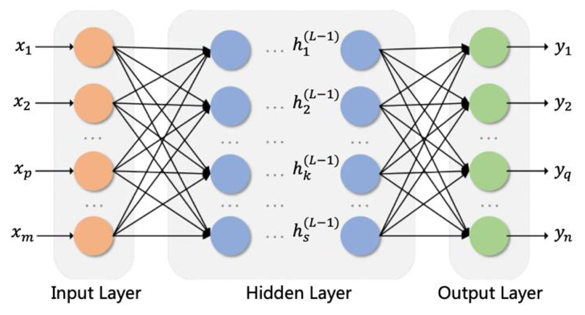
A BP neural network is a multi-layer forward network with strong computational power, which is constructed by stacking multiple hidden layers or combining multiple models. Each layer in the BP neural network consists of several neurons, and computation and weight updates in the neurons are used to achieve forward and backward propagation. The architecture of the BP neural network is shown in
Figure 1.
Based on the synaptic signaling of biological neurons, the neurons follow a certain functional computational approach to obtain the output. In forward propagation, the output of the previous layer is used as the input of the next layer in the activation function to obtain the prediction value. Then, in backward propagation, error is minimized, and the loss function is minimized by selecting the neural network weights.
Forward propagation:
It is assumed that the BP neural network is built with an input layer,
L hidden layers, and an output layer. The nonlinear relationship between the hidden layer
k and the neurons in the output layer is denoted as
hk (
k = 2, 3,…,
L + 2). The connection weight from the
hth neuron in the (
k − 1)th layer to the
tth neuron in the
kth layer is
. The sum of the
hth neuron input in the
kth layer is
and the output is
. They are defined as follows:
where
represents the total number of neurons in the (
n − 1)th layer,
k = 2, 3,…,
L + 2.
It is assumed that there are
m neurons in the input layer and
n neurons in the output layer. The input of the BP neural network is
, and the output data can be obtained from the input layer through each hidden layer node as follows:
Backward propagation:
In backpropagation, the gradient descent method is used to continuously update the weight along the negative gradient of the objective function so that the difference function between the desired output and the actual output of the neural network is minimized.
The specific formula is as follows:
where
is the update weight,
is the desired output,
is the actual output, and
is the learning rate, which is generally set to 0.5.
To achieve greater prediction accuracy, both the Kriging model and BP neural network are utilized in the surrogate model. They each play a different role. The Kriging model can be used to obtain the response of bubble density in the underwater bubble plumes. The second surrogate model is based on the BP neural network structure. The proposed BP neural network structure contains three neurons in the input layer, which correspond to the source leakage rate, the radius of the bubbles, and the bubble particle velocity, respectively. The hidden layer contains 30 neurons, and the output layer contains five neurons, which correspond to the bubble densities at the five observation points. When constructing a BP neural network model, the hyperparameters are crucial to the performance of the model. In this study, taking into account previous experience, the characteristics of the dataset, and the experimental training effect, the learning rate, the number of hidden layers, the activation function, the number of iterations, and other parameters of the network is determined after repeated adjustments and optimization.
2.4.3. Optimization Model
An optimization model usually consists of three components: decision variables, an objective function, and constraints. In this study, the decision variable is the bubble velocity in the bubble plume from the UNGP. The objective function is the minimum value of the difference function between the actual monitored bubble density and the bubble particle velocity. The constraint condition is that the bubble velocity at each monitoring point conforms to the velocity model and the radius of the bubbles contained in the plumes is within the reasonable range. The optimization model is shown as follows:
where
z is the objective function,
is the actual monitored value of the bubble radius in the
areath monitoring area,
is the simulated value of the bubble radius in the
areath monitoring area,
is the total number of monitoring areas.
where
v is the bubble particle velocity,
is the underwater bubble density in the monitoring area,
and
are the lower and upper bounds of the bubble radius, and
and
are the lower and upper bounds of the underwater bubble motion speed, respectively.
By solving the optimization model, the bubble velocity and bubble radius parameters can be obtained in accordance with the actual situation. When combined with the optical images, the bubble diffusion condition at the location described by the optical images of the underwater bubble plume can be effectively described. Based on the underwater bubble motion velocity, the distance between the leak source and the location of optical image acquisition can be inverse-determined based on the flow velocity. Furthermore, based on the bubble density in the underwater bubble plume, the volume of the leak source can be determined via inversion.
3. Results
3.1. Simulation Study Area Overview
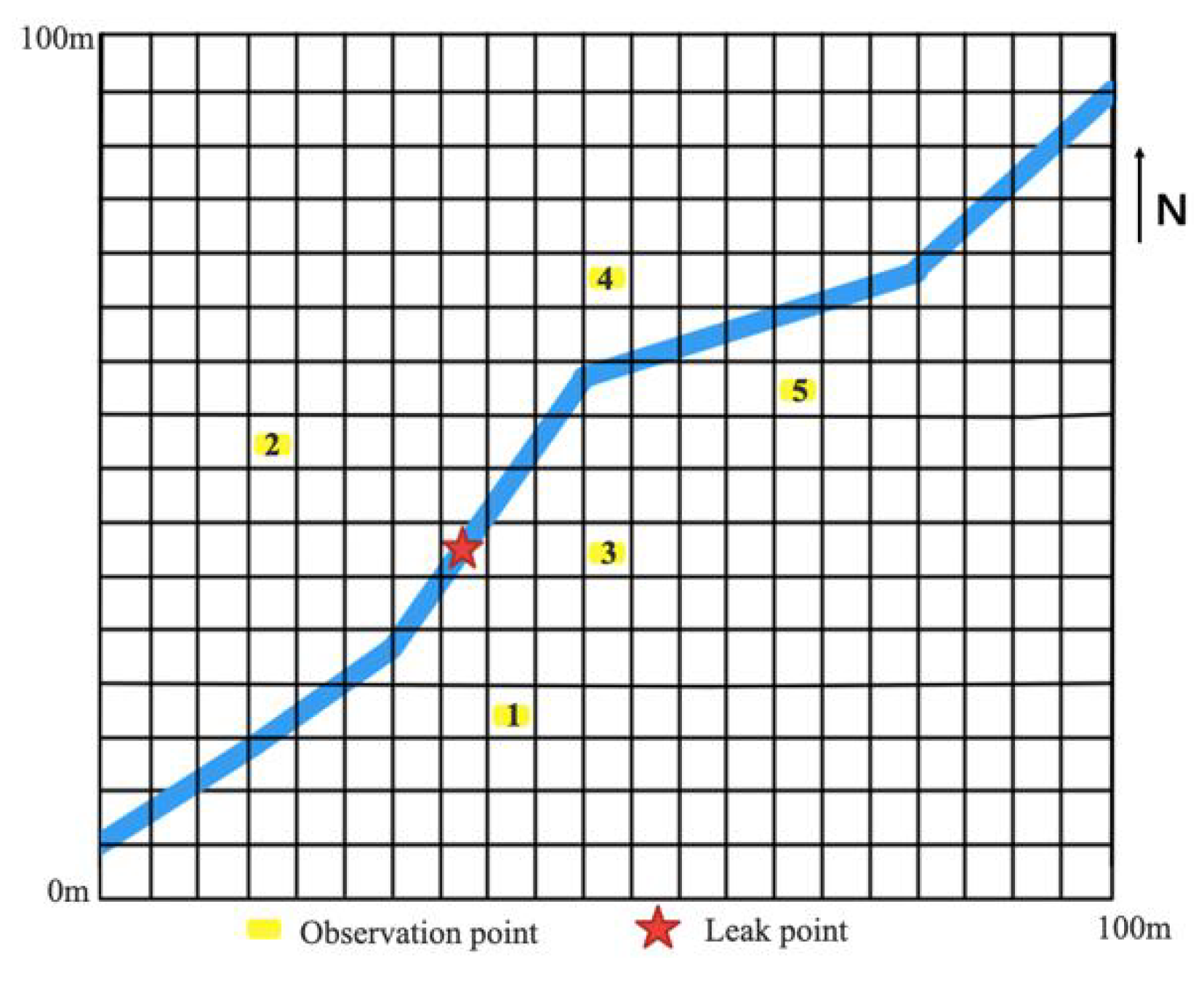
It is assumed that the size of the water area is 1000 m × 1000 m, and the depth is 20 m. The gas transmission pipeline was set at the bottom of the water, and a leak point was created on it. At the same time, five observation points were randomly established near the gas transmission pipeline, and the distance between each observation point and the water bottom was different. The test site layout is shown in
Figure 2. The blue line is the gas transmission pipeline, the yellow points are the five observation points, and the red star is the leak point.
Observation points were established on both sides of the underwater pipeline, with two on the left side and three on the right. The observation points have different depths. The different position and depth settings can ensure a more comprehensive view of the underwater bubble plume diffusion process. Furthermore, the fixed observation position ensures proportionality between the imaged target size and the real value, enabling later analysis and calculation.
With the help of a self-made autonomous underwater vehicle (AUV), some flow field information, such as the flow velocity, the depth, and the water temperature, can be obtained, and underwater bubble plume images can be taken near the observation points. In the testing environment, the direction of water flow is roughly from west to east. The flow field parameters determined through simulation model calibration are shown in
Table 1.
3.2. Numerical Modeling and Solving
The Discrete Random Walk Model and the k-epsilon Viscous Model in FLUENT are utilized to solve the two numerical models proposed in this study. After careful parameter adjustment and fitting, a simulated image of bubble plume diffusion at each observation point is obtained (shown in
Figure 3).
The deeper the water at the observation point, the greater the density of the bubble plume. At observation point 1, the water is the deepest; it is relatively close to the pipeline, and it is very close to the leakage port, so both the number of bubbles and the bubble density are the highest. At observation point 2, the water becomes shallower, and the location is far from the pipeline and west of the leak, which is opposite to the direction of the current. Therefore, the bubble plume density at observation point 2 is much lower, and the number is significantly reduced. Observation points 4 and 5 are both far away from the leakage port, but because they are east of the leak, bubble plumes can still be observed along the water flow. The number of bubble plumes that can be seen at observation point 5 is much higher than at observation point 4 because the water is much deeper. On the other hand, observation point 4 is closer to the water surface and far from the leak source, so the bubble plume observed at this location contains the lowest number of bubbles and is the least dense.
By using the underwater bubble diffusion velocity model, the observed and simulated values of the average underwater bubble motion velocity at each observation point are obtained, as shown in
Table 2. At the same time, by solving the bubble radius model, the average observed and simulated bubble radii are found; they are compared in
Table 3.
In order to describe the degree of agreement between the simulated and measured values, the absolute deviation (AD) and relative deviation (RD) are calculated. As for the average bubble velocity and bubble motion velocity, the error is very small for all observation points. Among them, observation point 3 is very close to the pipeline and the leakage point, so the simulation is the best; both observation points 4 and 5 are far from the leakage site and the pipeline, and the bubble diffusion process is influenced by many factors, so the simulation results deviate significantly.
Compared to the bubble velocity model, the error in the bubble radius simulation is much larger. Since the measurement of bubble size according to the optical image has a large correlation with the shooting distance, an image captured far from the target is much smaller in size than an image captured at close range. This results in larger error. As can be seen from the location of the observation points, observation points 1 and 2 are far away from the pipeline; in particular, observation point 2 is not only about 20 m away from the pipeline but is also in the opposite direction of the water current. Therefore, the quantity of bubbles captured is low, and the bubbles are small, causing a significant deviation compared to the simulation results.
In summary, after continuous correction of the model parameters, the average RD of the bubble motion velocity between the calculated and measured values is 8.44%, and the average RD of the bubble radius between the calculated and measured values is 24.96%, indicating that the calibration result is satisfactory. Observation points #1 and #2 are far away from both the pipeline and the leak and are located opposite the direction of leak spread, resulting in a large average relative error when predicting the radius of the bubbles. The predictions at the other observation points are more accurate. Therefore, it is proven that the choice of the observation point has a great influence on the test results. Furthermore, if the observation points are set reasonably, the calculation accuracy can be improved, and better results can be obtained.
3.3. Prediction Results Simulation
Based on the calibrated flow field parameters, it is feasible to apply the proposed underwater bubble plume diffusion numerical model to predict the spatial and temporal distribution characteristics of bubble plume diffusion in the study area. Taking the current underwater environment as the initial condition, the spatial and temporal distribution characteristics of future bubble plumes can be predicted.
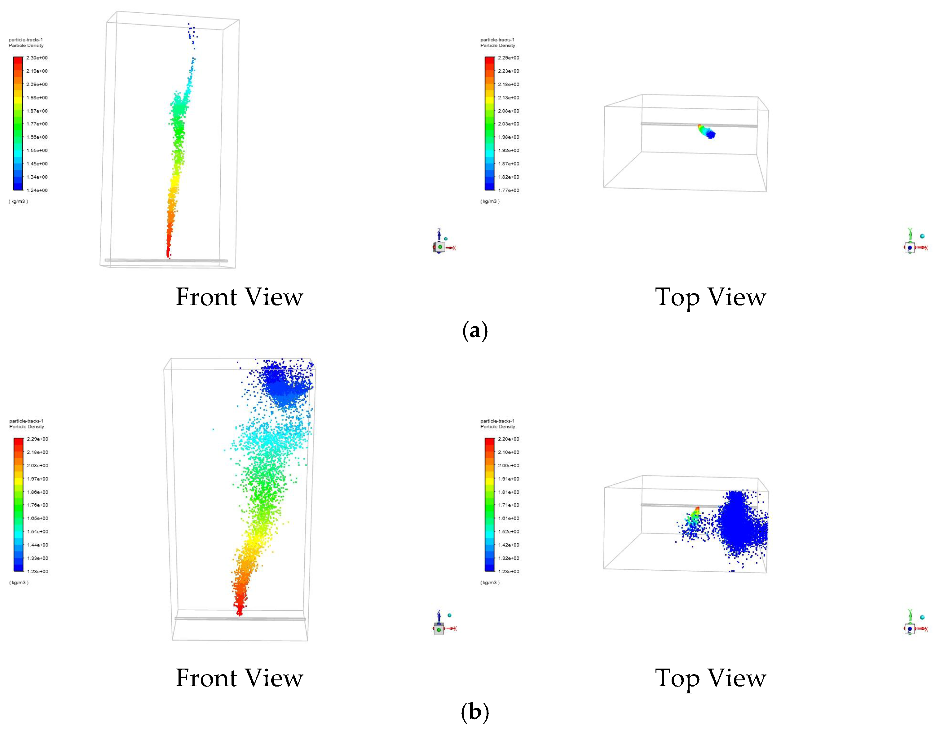
It has been proven that the VOF model in FLUENT can accurately simulate the overall pattern of underwater gas plume motion and the motion trajectory of discrete particles of bubbles during gas leakage [
35]. In order to verify the relationship between the bubble radius, bubble motion velocity, and flow field environment, we designed a VOF model of bubble plume motion in a wave field and simulated the diffusion of a single bubble list in water. In the proposed numerical model, the direction of water flow is set from left to right, the speed is 0.5 m/s, and the water depth is about 18 m.
In order to show the diffusion of the underwater bubble plumes more comprehensively, a bubble diffusion simulation was carried out for different dimensions. For the underwater movement of the individual bubbles, a two-dimensional simulation was utilized to illustrate the changes in each detail in the underwater diffusion process. For the overall diffusion of the total bubble plumes, a three-dimensional simulation was used to more clearly show the complete process of the formation and motion of bubble plumes from the leakage point to the air interface.
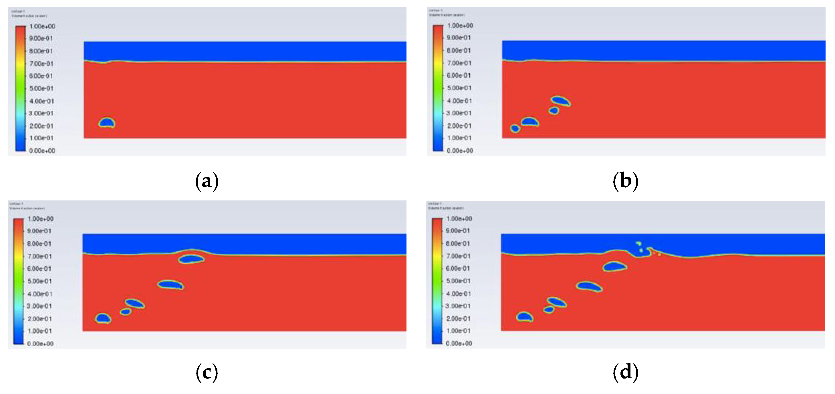
It is assumed that only one bubble leaks at a time. The bubbles leaking from the origin are shown in
Figure 4. It is clear that the first bubble will reach the water surface in about 5 s, and the bubbles will spread to a position approximately 4.2 m away from the leak point. Meanwhile, from the leakage point to the water surface, the size of the bubbles will increase gradually, and the radius of a bubble that is about to reach the water surface increases by about 125% compared to the radius of a bubble at the leakage source. It is important to note that the main aim of the experiments shown in
Figure 4 was to quantitatively test the diffusion distance, and the simulation results regarding changes in bubble size can only be qualitatively analyzed. In order to ensure the accuracy of the identification results, both the simulation results and the real underwater image features are crucial.
Due to the hydrodynamic influence of convective factors on the migration of underwater bubble plumes, the migration direction of the bubble plumes is basically consistent with the water flow direction. Throughout the entire simulation period, both the surface diffusion area and the flow offset distance of the bubble plumes gradually expand over time. At the fifth second, the bubble plumes are slowly drifting eastward with the water flow and have not yet reached the surface. At this time, the maximum flow deflection distance of the bubble is about 2.5 m. At the 10th second, the bubble plumes continue to deflect eastward, and the maximum flow deflection distance is about 5.5 m. At this time, the bubbles have spread to the water surface, and the area of the bubbles spread on the water surface is about 1.13 m2.
With continuous breaking, reorganization occurs during bubble diffusion, and most of the bubbles will break completely when they reach the surface of the water. As seen in
Figure 5, when the diffusion time is greater than 20 s, the flow deflection distance and the bubbles’ spread area are no longer very large. The maximum flow deflection distance is about 30 m, and the area of bubble spread on the water surface is about 3.5 m
2.
3.4. Inverse Solution of Leakage Source Parameter
Five observation points and a leakage point were set up in the study area, as shown in
Figure 1. The monitoring data obtained at each observation point are considered the known conditions. They are required to inverse the key leakage source parameters using the proposed simulation–optimization approach.
3.4.1. Surrogate Model Accuracy Verification
The Kriging surrogate model and BP neural network surrogate model were developed to act as surrogates for the complex numerical model of underwater bubble plume diffusion. In order to build the high-precision Kriging surrogate model, the number of sampling groups
should satisfy the following condition:
where
denotes the number of variables to be solved.
The coefficient of determination (
R2) and the mean relative error (MRE) are utilized to measure the accuracy of the proposed surrogate models.
where
is the sum of squared regression errors, and
is the sum of squared total errors.
where
is the number of sampling groups,
is a sample in the group,
refers to the output of the numerical model, and
is the output of the surrogate model.
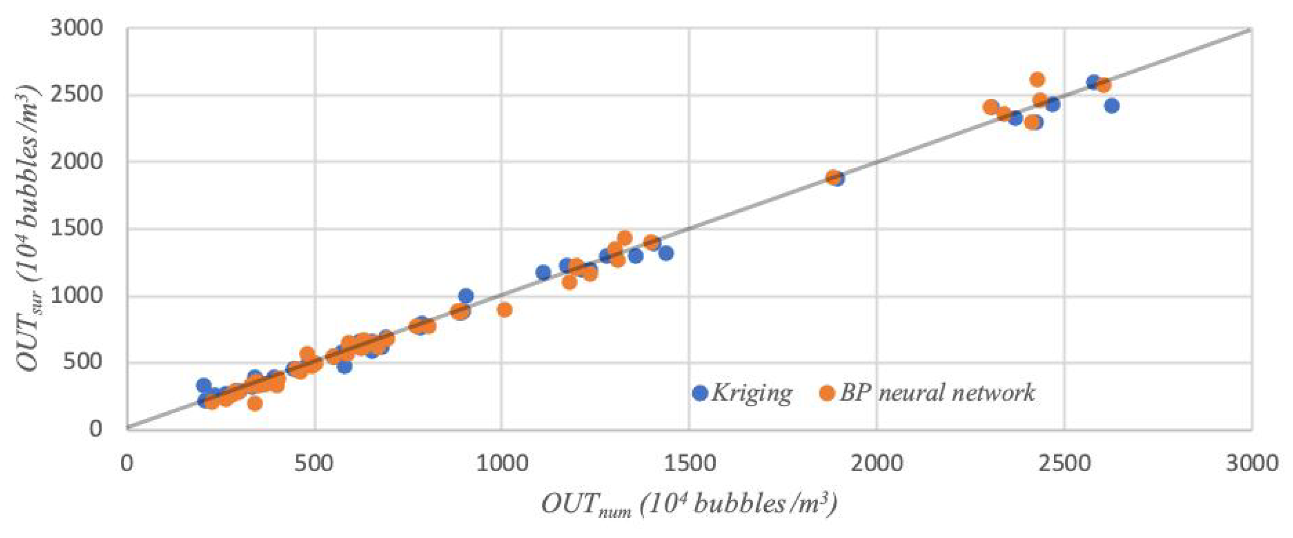
The flow field parameters collected at the five observation points and the data obtained from the underwater optical images are fed into the surrogate models, and the bubble density at the five observation points is the output of the surrogate models. At the same time, 50 datasets are randomly selected to build simulation training samples, and another 10 sets of test group samples are obtained to verify the accuracy of the proposed surrogate models (
Figure 6).
As seen in
Table 4, the MRE of the Kriging model is much smaller at only about 5.39%. Overall, both models achieve good performance, but the fitting accuracy of the Kriging model is slightly better than that of the BP neural network model.
3.4.2. UNGP Leakage Source Key Parameter Inversion
In this study, based on the data collected at each observation point, as shown in
Figure 2, an optimization model for the inverse identification of the bubble particle velocity
v and the underwater bubble density
is constructed. In the proposed model, the objective function is the minimization error between the simulated values and the actual observed values, and the decision variables are
v and
. The surrogate model of the numerical model is embedded into the optimization model in the form of constraints, which are also used as the decision variables.
During the test, the optimization model constructed is as follows:
where
z is the objective function,
is the actual monitored value of the bubble radius in the
areath monitoring area,
is the simulated value of the bubble radius in the
areath monitoring area.
The optimized model was solved using the simulated annealing algorithm, and the calculated identification values of the two methods are shown in
Table 5. The optimized model achieves better inversion results. Based on the Kriging surrogate model, the relative errors of the leakage key parameter inversion for both the leakage speed and the deflection distance are no more than 12%, and the running time is 13 min. Meanwhile, based on the BP neural network surrogate model, the relative errors in the leakage speed and the deflection distance are 13.9% and 15.3%, respectively, and the running time is 2.5 min.
In a comprehensive comparison, although both methods can achieve high inversion accuracy, the Kriging surrogate model fits the numerical model with higher accuracy, while the BP neural network surrogate model is much faster. In summary, both simulation–optimization methods, each based on one of the two surrogate models, can effectively complete the parameter inversion. This result is extremely important for leak risk assessment and underwater leak source location detection.
Finally, key engineering parameters such as the location of pipeline corrosion and estimations of leakage volume can be determined using the offset distance and leakage speed. Based on the image-acquisition position, offset distance, and pipeline arrangement scenario, the range of the leak location can be estimated, which greatly reduces the difficulty and effort required in positioning. The leakage volume can be estimated based on the pressure inside the pipeline, the pressure outside the pipeline, and the leakage velocity, which provide the basis for the loss calculation.
4. Discussion
This study has proposed a stable and effective method for the comprehensive identification of UNGP leakage information. It has identified that the simulation–optimization methods have a positive effect on the parameter inversion performance. Both the method based on the Kriging surrogate model and the method based on the BP neural network surrogate model can achieve satisfactory fitting accuracy. The optimization model based on the Kriging surrogate model can achieve higher inversion accuracy, while the optimization model based on the BP neural network surrogate model requires less calculation time.
In the proposed method, the underwater bubble diffusion velocity model and the bubble radius model, as well as optical images, are utilized to calibrate the flow field parameters. Therefore, a more accurate numerical simulation model can be established. Moreover, to the best of our knowledge, a suitable method for the inverse identification of UNGP leakage sources using the underwater bubble plume diffusion law and optical image analysis has not been proposed before; therefore, our estimations may generate novel concepts for the traceability and maintenance of underwater pipeline leakages.
It should be noted that this study is limited in its generalization of findings due to the complex underwater environment examined. The experimental environment of this study was a natural lake on campus with clear water and a gentle flow, and the fluid environment was very stable. Therefore, the motion of bubble plumes in such an environment is relatively regular. This is convenient for numerical simulation and simulation, and accurate inversion results can be obtained. However, there are more complex water environments with more disturbed flows in nature. Moreover, the underwater environment is more complex under extreme conditions such as floods and storms. The results of this study are not applicable to inversion calculations in such underwater environments.
Furthermore, the quality of underwater optical images obtained in this study also affected the inversion calculation accuracy. As mentioned before, the position and the distance at which optical images are captured can affect the analysis results. Blurry bubble plume images captured in a turbid underwater environment do not facilitate the analysis and calculation of bubble plume parameters. Therefore, in this study, optical images taken in clear water and close to the bubble plumes were favorable for obtaining accurate calculation results. If the shooting conditions are poor, the inversion accuracy will be seriously affected.
5. Conclusions
This study proposes a multi-model collaborative inversion framework for UNGP leakage source identification. Furthermore, an integrated method comprising fluidics and artificial intelligence is developed for application in a complex underwater environment. It can be utilized to trace underwater diffusion targets and survey sources.
In the future, more research on high-quality underwater bubble plume image obtainment and complex underwater environment intelligent modeling will be conducted. The focus of this study was mainly on underwater bubble images. Unfortunately, many underwater images are not clear enough; therefore, we plan to develop an improved high-quality method for obtaining underwater bubble plume images with high-definition underwater capture and intelligent image preprocessing so that the quality of the basic data can be effectively improved.
Moreover, to ensure that the results of the framework are dependable, various complex changes in the underwater environment need to be considered; for this purpose, designing intelligent modeling methods is necessary. The discrete phase model in FLUENT does not consider the breaking or coalescence of bubbles, which was one of the reasons for error in the prediction results. We will carry out more in-depth studies in the future to fully consider the influence of this factor on the prediction so as to improve the prediction process and increase the prediction accuracy. Finally, this study only focuses on the technological aspects of UNGP leakage source inverse identification. In future studies, we intend to conduct additional research on images of underwater bubble plume localization. Moreover, we will strive to obtain the coordinates of the leak source and provide accurate localization for pipeline repairs.
Based on this simulation–optimization approach to the inverse identification of UNGP leakage sources, these sources can be studied. Adopting a similar research focus and taking into account the oil underwater diffusion movement law, we intend to develop more intelligent underwater target recognition and source localization methods.


