Insights to Estimate the Largest 1/3, 1/10, and 1/100 of Offshore Wave Heights and Periods Under Fetch-Limited Conditions in the Central Aegean Sea

Abstract

The objective of this study is to compare the most common methods for forecasting wave characteristics (height and period) for the maximum in height 1/3, 1/10, and 1/100 of the waves, using available wind and wave datasets. The testing marine region is the Central Aegean Sea and, in particular, the east coast of Evia Island that is exposed to N, NE, E, and SE incoming offshore waves. The estimated values of wave characteristics resulting from three different wind datasets and the two wave datasets present differences of 2–60%. These variations are attributed to the different methodological approaches followed, to the different types of raw data in terms of space and time periods, and to the fetch limitations. The proposed methodology for the calculation of wave characteristics for the highest (1/10) and (1/100) waves appears to yield reasonable outcomes when compared to the corresponding significant (highest 1/3) wave heights and periods. Finally, mean values of wave height and period calculated from the five available datasets, considering their standard deviation, seem to be more representative than the values calculated separately from each dataset.

1. Introduction

Wave characteristics have been shown to exert a significant influence on the evolution of coastal morphology [1]. This is due to their application in a variety of contexts, including open-sea navigation, the quantification of wave energy potential, and the provision of necessary information for coastal engineers and researchers. This information is essential for the development of coastal structures and the maintenance of the resilience of coastal zones [2].

Conventionally, wave characteristics (i.e., height, period, direction) are calculated using data primarily from ground-based (coastal) meteorological stations. This approach has been the predominant one employed for several decades, extending up to the present day. Since the early 1970s, however, the use of buoys and other instruments to conduct in situ measurements of wave characteristics has become increasingly commonplace, while in the late 1970s satellite radar altimeters began providing open sea wave measurements. Since the beginning of the 20th century, offshore wave characteristics originate from global observation (e.g., TOPEX POSEIDON) and global reanalysis datasets [3] (e.g., ERA-40, ECMWF ERA-Interim). In the Mediterranean Sea, the initial investigation into the correlation between wind fields and wave development was conducted by Cavaleri et al. [4]. Subsequently, Llionelo and Sanna [5] examined the relationship between Mediterranean wave climate and the North Atlantic Oscillation (NAO) and the Indian Monsoon atmospheric systems. As stated by Stefanakos et al. [6], wave statistics for the entire basin have been produced within the framework of the MEDATLAS project, utilizing historical data from the ECMWF archives and satellite data (Topex altimeter). In a recent study, Barbariol et al. [7] presented a climatology of wind waves for the entire Mediterranean region. This study was based on a 40-year wave hindcast, which was produced by combining ERA5 Reanalysis of wind forcing with the State-of-the-Art WAVEWATCH III spectral wave model. The study was verified against satellite altimetry. A number of studies have been conducted on specific marine regions of the Mediterranean Sea, including the NW Mediterranean [1,8,9], Tyrrhenian [10], Adriatic [11,12], SE Mediterranean [13,14,15], Aegean Sea [16].

All the aforementioned studies refer to offshore wave conditions in marine regions wherein fetch distances do not play an important role in wave development. However, in the case of the Aegean Sea, fetch distances vary dramatically when they refer to particular coastal sectors. This is due to the diverse configuration of the coastline and the presence of more than 1520 islands and islets. This complexity is particularly pronounced in the central Aegean Sea. Consequently, coastal studies continue to utilize wind-generated offshore wave hindcasts, employing wind data for such analyses [17,18], while during the last decade, wave metadata have been available from the Copernicus Mediterranean Sea Waves Reanalysis (https://data.marine.copernicus.eu/, accessed on 12 May 2024), except for some semi-enclosed marine embayments (e.g., Korinthiakos Gulf, Amvrakikos Gulf, Paggasitikos Gulf). Moreover, low-resolution satellite data may lack the detail needed for precise wave analysis, while high-resolution observations, which offer greater accuracy and spatial detail, remain costly and resource-intensive for constant monitoring [19].

In relation to the constraints imposed by fetch limitations, data availability, and associated costings, the aim of this paper is to provide a useful approach to coastal geologists, oceanographers, and engineers for the prediction of the characteristics of the offshore waves approaching the coast. This will be achieved by utilizing the available wind and wave datasets and the most common hindcasting methods. The primary objectives of this study are as follows: (i) To examine the differences in the calculation of the fetch distances; (ii) To compare the most commonly used methods for predicting wave characteristics (height and period) from wind data, both for the significant values (the mean value of the largest 1/3 waves) and for the average values of the highest tenth (1/10) and hundredth (1/100) waves; (iii) To extract the average values for the largest 1/10 and 1/100 of the significant wave values provided by open-source wave datasets; and (iv) To compare the hindcasted wave values from the wind data with those provided by the open-source wave datasets.

2. Study Area

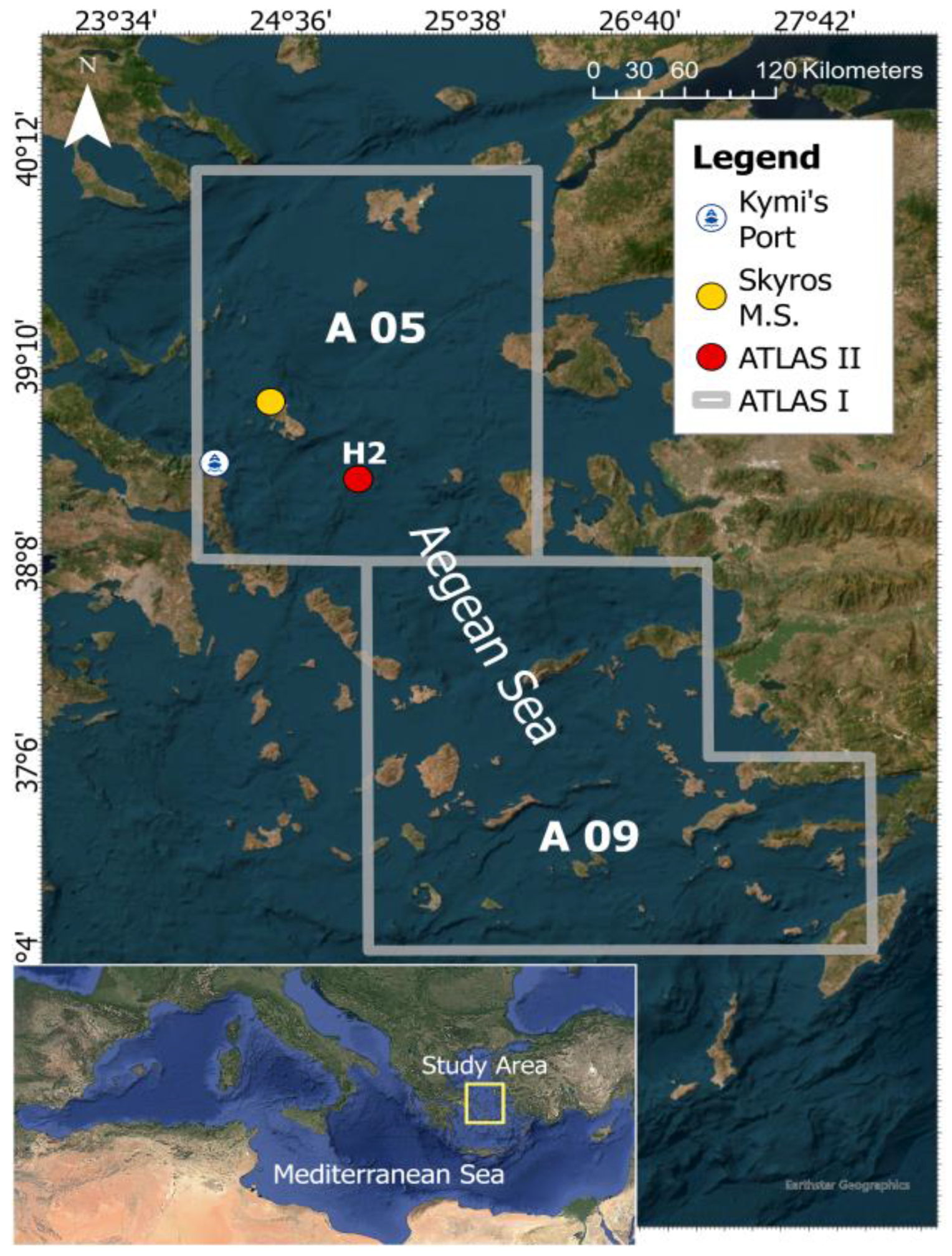
For the purposes of this study, the eastern coast of the island of Evia (Figure 1), in the vicinity of the port of Kymi (Figure 1), has been selected as the study area. This selection was made on the basis of the availability of various wind and wave datasets, as well as the significant variations in the fetch distances of the predominant wind/wave directions to which this coastal sector is exposed.

Off the coast of Kimy, the prevailing wind field is characterized in winter by strong northerly winds, with occasional southerly winds [20]. In spring, south-southwestern winds prevail, while in summer and the beginning of autumn, moderate to strong, cool and dry Etesian winds dominate. The latter blows northerly under clear skies, persists for long periods, and often reaches gale force.

The east coast of Evia (in the vicinity of the port of Kymi) is subject to wind-generated waves approaching from the N, NE, E, and SE directions (Figure 1). It is important to note that each direction is associated with a different fetch distance due to diverse coastline morphology and the presence of the Aegean islands. The offshore wave heights (H) are typically in the range of 0.8–1.2 m, with maximum values rarely exceeding 6 m. Correspondingly, the periods (T) range from 2–6 s, with maximum values less than 12 s (see [21,22]).

3. Data Collection and Methodology

This section includes the following: (i) the sources of the wind and wave data are described, along with the type and the format of the utilized datasets; (ii) the methodological approach for the calculation of the offshore wave characteristics (height and period) from the wind and wave datasets.

3.1. Wind and Wave Data Sources

The following data sources have been identified as relevant for this study: (i) the Hellenic National Meteorological Service (HNMS); (ii) the Wind and Wave Atlas of the North-eastern Mediterranean Sea [23]; and (iii) the Mediterranean Sea Waves Analysis and Forecast provided by the Copernicus Marine Service (ata.marine.copernicus.eu/product/MEDSEA_ANALYSISFORECAST_WAV_006_017).

The HNMS wind data originate from on-land meteorological stations, the majority of which have been operational since 1950. In terms of wind, these stations provide either hourly data (in major cities and at airports) or 3-hourly data for wind speed (in Beaufort scale) and for the eight main geographical directions, measured to an accuracy of 10°. In the present study, wind data were obtained from the coastal meteorological station located in Skyros Island (see Figure 1), delivering hourly data for the period 1955–2021.

The “Wind and Wave Atlas of the Northeast Mediterranean Sea” [23]—henceforth referred to as Atlas I—utilizes primary data from the British Meteorological Office (i.e., 269,408 for wind parameters and 233,387 for wave parameters) derived from visual observations made by Voluntary Observing Ships during their regular cruises between 1949 and 1988. The Atlas provides mean annual and monthly values of occurrence over elementary regions (1 × 1 degree) for different ranges of wind speed (in knots) corresponding to the eight main geographical directions. In the case of waves, however, it provides only ranges of significant heights against ranges of periods, which is not relevant to the direction of wave propagation.

The more recent “Wind and Wave Atlas for the Greek Seas” by Soukissian et al. (2007) [24]—henceforth referred to as Atlas II—provides mean annual and seasonal wind and wave data, covering a 10-year period (1995–2004) with a 3-h time step. The numerical simulation of the wind and wave regime over a 10-year period (from 1995 to 2004) with a 3-h time step was carried out with a 0.1° × 0.1° field grid analysis. In the calibration of the model, field (point) measurements at six specific locations collected during the operation of the POSEIDON system from 1999 to 2006 were taken into account.

The Copernicus platform (ERA5) provides hourly wind data (10 m above sea level) from a 0.25° × 0.25° gridded reanalysis that combines model data and observations. ERA5 is the fifth generation of ECMWF reanalysis, offering a consistent global dataset for the past eight decades. Wave characteristics for the Greek Seas are provided by the Copernicus Marine Mediterranean Reanalysis Model, developed and evaluated by the Hellenic Centre for Marine Research (HCMR) with a 2014 simulation. Based on the WAM model, the system uses two computational grids to accurately simulate remote swells entering the Mediterranean through the Strait of Gibraltar. Atmospheric forcing comes from ECMWF’s 10-m wind analysis, with a horizontal resolution of 1/8°.

3.2. Datasets

3.2.1. Wind Datasets

The wind data (i.e., wind speed and direction) required for offshore wave hindcasting were obtained from the meteorological coastal station on the island of Skyros, which is operated by the Hellenic National Meteorological Service (HNMS). The data were also obtained from Atlases I and II. The wind data from the Copernicus platform were not utilised due to its inclusion in the reanalysis for the hindcasting of the wind–wave characteristics.

The wind data from the Skyros meteorological station are presented in

Table A1. Mean annual frequencies of occurrence of wind speeds (in Beaufort scale) for the N, NE, E, and SE directions from the Syros meteorological station (for the period 1955–2021).

Beaufort	N (%)	NE (%)	E (%)	SE (%)
0	0.00	0.00	0.00	0.00
1	0.31	0.29	0.26	0.46
2	4.36	2.81	1.67	1.18
3	7.07	3.30	1.58	0.81
4	6.91	4.13	0.62	0.57
5	3.03	2.82	0.15	0.29
6	1.44	1.91	0.05	0.13
7	0.58	1.07	0.01	0.09
8	0.16	0.37	0.00	0.03
Total	23.92	16.76	4.36	3.58

of Appendix A; they include the annual frequency of occurrence of each class of wind speed (in Beaufort scale) for the main geographical directions.

The wind data abstracted from Atlas I are given as annual numbers of observations for each pair of wind speed ranges (in knots) and main geographical direction. For the N and NE directions, the data extracted from box AO2 were utilized, while for the E and SE directions, the average values from boxes AO2 and AO8 were calculated (see Figure 1). The dataset used in this study is presented in

Table A2. Mean annual numbers and frequencies of occurrence of wind speeds (U, in knots) for the N, NE, E, and SE directions, from the ATLAS I [23] boxes A2 and A8 (for locations see Figure 1) and for the period 1955–1988.

U (knots)	Number of Occurrences					Frequency (%) of Occurrence
	N	NE	E	SE		N%	NE%	E%	SE%
0.0	0	0	0	0		0.00	0.00	0.00	0.00
2.0	3	3	2	2		0.29	0.29	0.19	0.19
5.0	26	14	13	13		2.51	1.35	1.26	0.87
8.5	26	29	13	13		2.51	2.80	1.26	1.55
13.5	45	51	9	9		4.35	4.93	0.87	1.45
19.0	39	47	5	5		3.77	4.55	0.48	1.16
24.5	38	45	3	3		3.68	4.35	0.29	0.68
30.5	19	19	3	3		1.84	1.84	0.29	0.29
37.0	10	7	0	0		0.97	0.68	0.00	0.19
42.0	3	3	0	0		0.29	0.29	0.00	0.00
Annual Total	209	218	48	66		20.21	21.08	4.64	6.38

in Appendix A.

In the case of the Copernicus platform (ERA5), the obtained dataset is in the form:

-

u10-(eastward) component of the 10 m wind

-

v10-(northward) component of the 10 m wind

-

winddir_rad (wind (mathematical) direction in radians)

A sample from the aforementioned dataset is provided in

Table A3. A sample from the wind data from the Copernicus platform (ERA5).

Longitude	Latitude	Time	u10	v10	winddir_rad
24.2299995	38.58000183	1/1/1993 0:00	−3.26663	−1.93995	−2.60569438
24.2299995	38.58000183	1/1/1993 1:00	−3.97685	−1.82202	−2.71197558
24.2299995	38.58000183	1/1/1993 2:00	−4.05941	−1.96877	−2.69002509
24.2299995	38.58000183	1/1/1993 3:00	−4.30211	−2.79687	−2.56513548
…	….	….	…	…	…
24.2299995	38.58000183	31/12/2022 21:00	1.545489	−3.71157	−1.17623487
24.2299995	38.58000183	31/12/2022 22:00	2.021021	−3.47357	−1.04384502
24.2299995	38.58000183	31/12/2022 23:00	2.037818	−3.72427	−1.07012636

, which can be found in Appendix A.

3.2.2. Wave Datasets

The wave data were extracted from two sources, as mentioned earlier: (i) the Wind and Wave Atlas of the Hellenic Seas, referred to as Atlas II [24] (see Figure 1); and (ii) the Copernicus platform, from which hourly values were downloaded for the period 1 January 1993–31 December 2022.

The wave data extracted from Atlas II pertain to the offshore point H2 (see Figure 1) and comprise two tables elucidating the relationship between significant wave height (Hs) and peak period (Tp) (see

Table A4. Display of significant wave height Hs and wave period Tp from ATLAS II for the wider area of Kymi at point H2 (38.55° N and 25.00° E).

Tp		Hs														Total
Range	Mean Value	0.00–0.25	0.25–0.50	0.50–0.75	0.75–1.00	1.00–1.25	1.25–1.50	1.50–1.76	1.75–2.00	2.00–2.50	2.50–3.00	3.00–3.50	3.50–4.00	4.00–5.00	5.00–6.00
0.0–1.9	0.95	2	1	0	0	0	0	0	0	0	0	0	0	0	0	3
1.9–2.6	2.25	4	9	0	0	0	0	0	0	0	0	0	0	0	0	13
2.6–3.1	2.85	11	44	6	0	0	0	0	0	0	0	0	0	0	0	61
3.1–3.8	3.45	17	87	64	3	0	0	0	0	0	0	0	0	0	0	171
3.8–4.6	4.20	10	59	118	48	6	0	0	0	0	0	0	0	0	0	241
4.6–5.0	4.80	4	11	24	38	29	3	0	0	0	0	0	0	0	0	109
5.0–5.5	5.25	3	9	11	20	34	23	4	0	0	0	0	0	0	0	104
5.5–6.1	5.80	2	8	5	9	12	24	23	5	1	0	0	0	0	0	89
6.1–6.7	6.40	1	7	5	4	5	7	13	18	12	0	0	0	0	0	72
6.7–7.4	7.05	1	4	5	3	2	3	3	6	18	5	0	0	0	0	50
7.4–8.1	7.75	0	2	5	4	2	2	2	1	5	9	3	0	0	0	35
8.1–8.9	8.50	0	1	4	4	2	2	1	1	2	2	4	2	1	0	26
8.9–9.8	9.35	0	0	1	2	2	1	1	1	1	1	1	2	3	0	16
9.8–10.8	10.3	0	0	0	1	1	1	1	0	0	0	0	0	1	2	7
10.8–11.9	11.35	0	0	0	0	0	0	0	0	1	0	0	0	0	0	1
Total		55	242	248	136	95	66	48	32	40	17	8	4	5	2	998

in the Appendix A) and significant wave height with the dominant geographical direction per 15 degrees (see

Table A5. Significant wave height (Hs) and wave direction (Θw) from ATLAS II at point H2 (38.55° N and 25.00° E).

Hs→	0.00–0.25	0.25–0.5	0.50–0.75	0.75–1.00	1.00–1.25	1.25–1.50	1.50–1.76	1.75–2.00	2.00–2.50	2.50–3.00	3.00–3.50	3.50–4.00	4.0–5.0	5.0–6.0	Total
Θwave↓
345	3	17	22	8	3	2	1	1	0	0	0	0	0	0	57
0	5	18	28	19	16	12	9	6	7	3	1	0	0	0	124
15	6	15	22	16	14	13	10	11	16	8	4	3	4	2	144
30	5	8	7	4	3	2	1	1	1	1	0	0	0	0	33
45	1	3	4	2	1	0	0	0	0	0	0	0	0	0	11
60	0	2	2	1	0	0	0	0	0	0	0	0	0	0	5
75	0	1	1	1	0	0	0	0	0	0	0	0	0	0	3
90	1	2	1	1	0	0	0	0	0	0	0	0	0	0	5
105	1	2	3	1	1	1	1	0	0	0	0	0	0	0	10
120	1	3	5	3	1	1	1	0	0	0	0	0	0	0	15
135	1	4	5	3	2	2	1	1	1	1	0	0	0	0	21
150	1	5	10	6	5	4	3	2	2	2	1	0	0	0	41
Grant Total	54	242	248	136	94	67	47	31	35	17	6	3	4	2	986

in the Appendix A).

The hourly wave data from the Copernicus database refer to the period 1 January 1993–31 December 2022 and include the time series (see

Table A6. A sample from the wave data from the Copernicus platform (MED_wave).

01/1993–12/2017	Latitude	Longitude	VHM0	VMDR	VTM01	VTPK
1/1/1993 0:00	38.5625	24.25	0.128	59.33	1.583	2.434
1/1/1993 1:00	38.5625	24.25	0.205	66.00	1.870	2.348
1/1/1993 2:00	38.5625	24.25	0.250	64.46	2.003	2.347
1/1/1993 3:00	38.5625	24.25	0.324	59.77	2.204	2.367
…	…..	…	…	….	…	….
31/12/2017 22:00	38.5625	24.25	0.013	267.68	0.981	2.654
31/12/2017 23:00	38.5625	24.25	0.000	180.00	1.000	2.640

, in Appendix A). VHM0_WW:

Spectral significant wind wave height:

VTM01_WW:	Spectral moments (0.1) wind wave period (Τm01)
VTPK:	Wave period at spectral peak/peak period (Tp)
VMDR_WW:	Mean wind wave direction

3.3. Methodology

In order to facilitate the objectives of the present investigation, the wave characteristics (H and T) have been calculated for the highest 1/3, 1/10, and 1/100 of the waves using both existing wind and wave data, as presented earlier.

3.3.1. Calculation of Wave Characteristics from Wind Data

Methodologically, the two widely used approaches for calculating wave characteristics from wind data are as follows: (i) the SMB (Sverdrup–Munk–Bretschneider) method, as outlined in the Shore Protection Manual [25]; and (ii) the JONSWAP method, derived from the Joint North Sea Wave Project (JONSWAP) [21] and subsequently presented in the U.S. Army Corps of Engineers [22].

Prior to the incorporation of wind speed data, the following prerequisite steps are mandatory:

(i)

The transformation of wind data given in different ranges and units (Beaufort, knots) to mean values expressed in SI units (i.e., m/s) as illustrated in

Table A7. The transformation of the wind speed ranges and mean values from Beaufort and knots into meters per second (m/s).

Beaufort	Knot	Knot (Range)	m/s	Mean Value (knot)	Mean Value (m/s)
1	1–3	0.51–3.5	0.262–1.830	2.0	1.029
2	4–6	3.51–6.5	1.831–3.346	5.0	2.572
3	7–10	6.51–10.5	3.347–5.404	8.5	4.373
4	11–16	10.51–16.5	5.405–8.491	13.5	6.945
5	17–21	16.51–21.5	8.492–11.063	19.0	9.774
6	22–27	21.51–27.5	11.064–14.150	24.5	12.604
7	28–33	27.51–33.5	14.151–17.236	30.5	15.691
8	34–40	33.51–40.5	17.237–20.838	37.0	19.034
9	41–47	40.51–47.5	20.839–24.439	44.0	22.636
10	48–55	47.51–55.5	24.440–28.552	51.5	26.494

of the Appendix A;

(ii)

The calculation of the average value of the height and period of the highest 1/3, 1/10, and 1/100 of the waves from the corresponding wind speeds is also required, with the latter to be calculated as a weighted average relative to their annual frequency of occurrence of the strongest 1/3, 1/10, and 1/100 of the winds in each main direction (i.e., N, NE, E, and SE) (see

Table A8. Calculations of the weight-averaged speed of the strongest 1/3, 1/10, and 1/100 winds.

Beaufort	U (m/s)	f (%)	f (1/3)	f (1/10)	f (1/100)
0	0.10	0.003
1	0.90	0.288
2	2.45	2.808
3	4.40	3.303
4	6.70	4.135
5	9.35	2.823	2.188
6	12.30	1.908	1.908	0.185
7	15.4	1.069	1.069	1.069
8	18.95	0.369	0.369	0.369	0.116
9	22.60	0.052	0.052	0.052	0.052
Total		16.757	5.586	1.676	0.168
The calculated weight-averaged values
			U (1/3) *1	U (1/10) *2	U (1/100) *3
			12.273	16.054	20.080

Note: (*¹) U_1/3 = [(22.6 × 0.052) + (18.95 × 0.369) + (15.40 × 1.069) + (12.3 × 1.908) + (9.35 × 2.188)]/5.586 = 12.273. (*²) U_1/10 = [(22.6 × 0.052) + (18.95 × 0.369) + (15.40 × 1.069) + (12.3 × 0.185)]/1.676 = 16.054. (*³) U_1/100 = [(22.6 × 0.052) + (18.95 × 0.116)]/0.168 = 20.080.

in the Appendix A);

(iii)

The extraction of data from the Copernicus (ERA5) database, specifically concerning apnea, defined as values of U10 < 0.51 m/s (1 knot).

(iv)

The calculation of wind speed (U₁₀) from its eastward (u₁₀) and northward (v₁₀) components, using the following equation:

U₁₀ = √(u₁₀² + v₁₀²),

(1)

(v)

The calculation of the meteorological direction (metD) from the mathematical direction (mathD) as follows:

-

If mathD < 270°, then metD = 270° − mathD

-

If mathD > 270°, then metD = 360 + 270° − mathD

(vi)

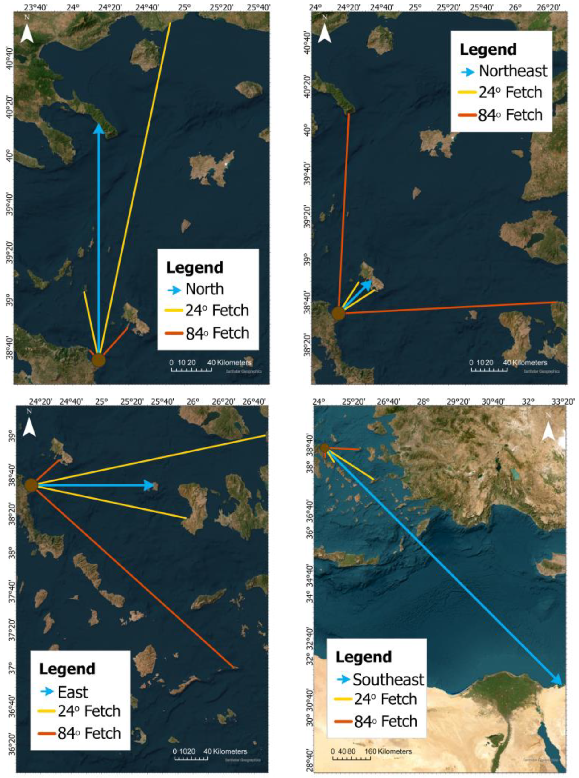
The estimation of the effective fetch (F_eff) of each primary wind/wave direction. In this study, the following two approaches were used (see Figure 2): (a) The arithmetic mean of nine distances [26], including the main direction and four other directions on either side of it, at an interval of three degrees (arc = 24 degrees) (Equation (2)); and (b) The consideration of seven rays on either side of the main direction, at a 6-degree interval (arc = 84 degrees) [27] applying Equation (3):

$$F_{eff}={\displaystyle \frac{{\sum }_{i=-N}^N{F}_i }{{\sum }_{i=-N}^{N}2{\rm N}}},$$

(2)

$$F_{eff}={{\displaystyle \frac{{\sum }_{i=-N}^N{F}_i \left(cos a_i\right)}{{\sum }_{i=-N}^N\left(cos a_i\right)}}}^2,$$

(3)

SMB Method

In accordance with the SMB method [25], the values of the wave characteristics of the significant wave height, the period, and the time required for the wind forcing to attain their maximum values are presented in

Table 1. Prediction equations for the significant wave height (Hs), the peak period (Tp), and the minimum wind duration (t) required to form their maximum values.

A. Fully Developed Wave Conditions		B. Fetch-Limited Wave Conditions
Hs = 2.4821·10−2·UA2	(4)	Hm = 1.616·10−2·UA·F1/2	(7)
Tp = 8.30·10−1·UA	(5)	Tp = 6.238·10−1·(UA·F)1/3	(8)
t = 2.027·UA	(6)	t = 8.93·10−1·(F2/UA)1/3	(9)

. The structure of this table comprises two columns; the left column corresponds to the case of fully developed wave conditions (i.e., independent of the fetch distance), whilst the right one corresponds to the case of fetch-limited wave development.

The U_A is given by the following relationship:

U_A = 0.71·U^1.23,

(10)

where (U) is the wind speed at the sea surface expressed as a function of measured wind speed at 10 m absolute height, with the (U₁₀) given by the following equation:

U = R_T·(U₁₀),

(11)

The amplification ratio (R_T) is dependent on the differences between the atmospheric (Ta) and the sea surface (Ts) temperature, as defined in CEM [25]. In the absence of temperature information, it should be assumed to be equal to 1.1. In the case that the meteorological station is located at an altitude (z), U₁₀ is given by the relationship:

U₁₀ = U_z·(10/z^0.143),

(12)

where (Uz) is the wind speed at altitude (preferably z < 20 m).

The selection of the set of equations A (fully developed) or B (fetch restricted) from Table 1 has been conducted in accordance with the following procedure: Initially, the time duration (t) required for the wind forcing to generate fully developed waves (Equation (6)) was calculated. Then, for this time, the minimum required fetch distance (F’) was determined using Equation (9). If F’ < F (F: actual geographical fetch), the set of equations for a fully developed sea (A) is used, and if F’ > F, the equations for limited fetch (B) are applied.

JONSWAP Method

The JONSWAP method [22] is based on the Pierson–Moskowitz wave energy spectrum, and its application involves the following steps.

The first step is to examine the inequality below:

$${\displaystyle \frac{g·F}{U_{10}^2}}>{\displaystyle \frac{34.528}{C_D}}$$

(13)

where (g) is the gravity constant, (U₁₀) is the wind speed at the sea surface, and (C_D) is the friction constant given by the following relationship:

$$C_D={10}^{-3}·(1.1+0.035·U_{10})$$

(14)

The second step checks whether the inequality in Equation (13) is satisfied. If the inequality in Equation (13) is satisfied, then the relationships (15) and (16) in

Table 2. Prediction equations of significant wave height (Hs) and peak period (Tp) according to the JONSWAP energy spectrum application.

A. Fully Developed Wave Conditions		B. Fetch-Limited Wave Conditions
Hs = (211.5 × Uw2)/g	(15)	Hs = 0.0413·Uw × (X/g)0.5	(17)
Tp = (239.8 × Uw)/g	(16)	Tp = 0.651 × [(Uw × X)1/3)/g2/3]	(18)

are applied.

If the inequality of relationship (13) is not satisfied (step three), meaning that fetch restriction is involved, then the inequality of relationship (19) is evaluated to determine whether the time duration (t_D) or the effective fetch (F) is the limiting factor:

$${\displaystyle \frac{gF}{U_w^2}}<0.0053·((g·t_D)/U_w{)}^{1.5},$$

(19)

where:

$$U_W=\sqrt{C_d·U_{10}},$$

(20)

and

$$t_D=77.23{\displaystyle \frac{F^{0.67}}{U_w^{0.34}{g}^{0.33}}},$$

(21)

If Equation (19) is satisfied, then Equations (15) and (16) in Table 2 are used, with X set equal to F (X = F). For the inverse scenario, the effective fetch distance (F’) that satisfies the time duration (t_D) is calculated from Equation (19) (considering it as equality) and, thereafter, the wave characteristics are calculated using Equations (17) and (18) in Table 2, for X = F’.

3.3.2. Calculation of Wave Parameters (H and T) from Wave Data

Different methodologies have been employed for each dataset, given its heterogeneity in terms of varying time steps and intervals in geographical direction.

Atlas II

To assign a distinctive Tp value to each Hs value in Table A4 of Appendix A, the peak period value is determined as a weighted average of the existing Tp values, relative to their frequency of occurrence, that corresponds to the same value of wave height. The calculated values are presented in

Table A9. The calculated weight-averaged values of peak period corresponding to significant wave heights (mean values), at point H2 (38.55° N and 25.00° E).

Tp Mean	Hs
	0.125	0.375	0.625	0.875	1.125	1.375	1.625	1.875	2.25	2.75	3.25	3.75	4.5	5.5
0.95	1.9	0.95	0	0	0	0	0	0	0	0	0	0	0	0
2.25	9	20.25	0	0	0	0	0	0	0	0	0	0	0	0
2.85	31.35	125.4	17.1	0	0	0	0	0	0	0	0	0	0	0
3.45	58.65	300.15	220.8	10.35	0	0	0	0	0	0	0	0	0	0
4.20	42	247.8	495.6	201.6	25.2	0	0	0	0	0	0	0	0	0
4.80	19.2	52.8	115.2	182.4	139.2	14.4	0	0	0	0	0	0	0	0
5.25	15.75	47.25	57.75	105	178.5	120.75	21	0	0	0	0	0	0	0
5.80	11.6	46.4	29	52.2	69.6	139.2	133.4	29	5.8	0	0	0	0	0
6.40	6.4	44.8	32	25.6	32	44.8	83.2	115.2	76.8	0	0	0	0	0
7.05	7.05	28.2	35.25	21.15	14.1	21.15	21.15	42.3	126.9	35.25	0	0	0	0
7.75	0	15.5	38.75	31	15.5	15.5	15.5	7.75	38.75	69.75	23.25	0	0	0
8.50	0	8.5	34	34	17	17	8.5	8.5	17	17	34	17	8.5	0
9.35	0	0	9.35	18.7	18.7	9.35	9.35	9.35	9.35	9.35	9.35	18.7	28.05	0
10.3	0	0	0	10.3	10.3	10.3	10.3	0	0	0	0	0	10.3	20.6
11.35	0	0	0	0	0	0	0	0	11.35	0	0	0	0	0
Total	3.69	3.88	4.37	5.09	5.47	5.95	6.30	6.63	7.15	7.73	8.33	8.93	9.37	10.30

of Appendix A.

The data presented in Table A5 (Appendix A) provide the mean annual frequency of occurrence for each pair of significant wave height and geographical direction at 15-degree intervals. For instance, in the case of NE direction (arc = 22.5–67.5°), frequencies of occurrence are given at three representative directions (i.e., 30°, 45°, and 60°) for each wave height interval. The mean value of the three frequency values corresponding to the NE direction is then calculated.

Table A10. Annual frequency of occurrence of the significant wave height (Hs, in m) that corresponds to the main geographical directions (N, NE, E, SE), at point H2 (38.55° N and 25.00° E).

	Hs
	0.125	0.375	0.625	0.875	1.125	1.375	1.625	1.875	2.25	2.75	3.25	3.75	4.5	5.5	Total
N	1.42	5.07	7.30	4.36	3.357	2.74	2.03	1.83	2.33	1.12	0.51	0.30	0.41	0.20	32.96
NE	0.61	1.32	1.32	0.71	0.41	0.20	0.10	0.10	0.10	0.10	0.00	0.00	0.00	0.00	4.97
E	0.20	0.51	0.51	0.30	0.10	0.10	0.10	0.000	0.00	0.000	0.00	0.00	0.00	0.00	1.82
SE	0.34	1.23	2.03	1.22	0.81	0.71	0.51	0.30	0.30	0.304	0.10	0.00	0.00	0.00	7.81
Total	2.54	8.11	11.16	6.59	4.66	3.75	2.74	2.23	2.74	1.521	0.61	0.30	0.416	0.20	47.56

in Appendix A presents the calculated mean frequencies of occurrence of significant wave heights for the four geographical directions.

COPERNICUS Platform

In order to determine the percentage of calm sea conditions, the proportion percentage of hourly values corresponding to both VHM0 < 0.064 m and VTM01 < 1 s is calculated from the total hourly values. Subsequently, the value parameters (VHM0, VTM01, VTPK, VMDR) are selected for each directional arc corresponding to each of the four main geographical direction sectors (as previously described).

Subsequently, to calculate the significant wave height Hs (H1/3) and peak period Tp (1/3), the average of all values in columns 1 and 2 (

Table 3. Columns 1 to 4 present the hourly values of significant wave height (Hs), peak Period (Tp), direction of wave propagation (DIR), and mean period (Tm). Column 5 gives the number of waves (N) while column 6 gives the cumulative number of waves (S(N)). All columns are arranged in a descending order, commencing with the highest wave height and concluding with the lowest.

1	2	3	4	5	6
Hs (m) (VHM0)	Tp(s) (VTPK)	DIR (°) (VMDR)	Tm (s) (VTM01)	N	S(N)
5.19	9.23	377.81	7.30	493	493
5.19	9.23	379.77	7.13	505	998
5.09	9.23	376.51	7.32	492	1490
5.03	9.23	376.67	7.31	493	1983
…	…	…	…	…	…
4.95	9.23	376.61	7.30	494	2476
4.92	9.24	376. 80	7.30	484	2960
Total number of waves:					9099

Note: The values of (N) and S(N) are given in integer form.

) is calculated. With regard to the direction of wave propagation (DIR), the median value is preferred over the mean, as the former more accurately represents the central tendency of directional data. However, it should be noted that there is only a small difference between the two; the values are only slightly different.

The calculation of the wave characteristics corresponding to the highest 1/10 and 1/100 of the wave dataset is achieved through the following procedure. Assuming that VTM01 in the original dataset represents the mean wave period, the number of individual waves within a one-hour interval can be estimated by dividing the total duration of one hour (3600 s) by the VTM01 value (see Table 3). The cumulative wave number for each successive hour is then calculated, and the total number of waves for the entire dataset is provided at the end. The number of waves that correspond to the highest 1/10 and 1/100 of the waves can be depicted from column 6 (Table 3). To illustrate this, consider a scenario where the total number of waves is 9099. In this case, the highest 1/10 of the waves corresponds to 909 waves, while the highest 1/100 corresponds to 91 waves. Subsequently, the calculation of the average value H(1/100), T(1/100), and the median of Dir(1/100) is conducted for all values greater than those corresponding to the data line wherein S(N) = 909. The same procedure is repeated for the highest 1/100 of the waves (i.e., S(N) = 91).

The final values of H(1/10) and H(1/100) are calculated using the following relationships, according to Rayleigh’s narrow band spectrum theory (Bretschneider, 1964) [28]:

H_1/10 ≈ 1.27·H_s,

(22)

H_1/100 ≈ 1.67·H_s,

(23)

The T(1/10) and T(1/100) values are calculated using the relationship (e.g., Goda, 2000) [29]:

T_1/10 ≈ T_1/100 ≈ 1.2·T_mean (Tm_0.1),

(24)

The frequency of occurrence is calculated on the basis of the number of waves that correspond to 1/3, 1/10, and 1/100 of the highest waves divided by the total number of waves (S(N)).

4. Results

The effective wave fetch lengths for the four wave approach directions toward the Kymi coast, calculated using the Smith [26] and SPM [27] methods, are presented in

Table 4. Fetch distances (F, in km), calculated for the four geographical directions, relative to the coast of Kymi (for location see Figure 1) using the three different methodologies.

	N	NE	E	SE
F (24°) (after Smith [26])	89.0	42.2	183.7	295.0
F (86°) (after SPM [27])	87.0	119.6	149.0	171.7
F (24°) minus F (84°)	+2.0	−77.4	+34.7	+123.3

. As is evident from the table, calculations based on the 24° arc yield greater distances than those based on the 86° arc, except for the NE direction, where a smaller value is obtained and a significant deviation is observed. These discrepancies are attributed to the complex coastal topography, which results from the presence of numerous small islands.

The frequency (in percentages) of the occurrence of the incoming offshore waves from the four geographical directions (N, NE, E, SE) for the different databases is presented in

Table 5. Mean annual frequencies (%) of waves approaching the coast of Kymi from the four main directions (N, NE, E, and SE) for the five databases.

Database	N	NE	E	SE
A. Skyros M.S._wind	23.92	16.76	4.36	3.57
B. Atlas I_wind	20.48	21.08	4.64	6.38
C. Copern._wind	35.96	12.73	4.28	4.68
D. Atlas II_wave	32.96	4.97	1.83	7.81
E. Copern._wave	19.23	10.39	2.59	4.45

. It is evident that all datasets provide average wind/wave frequencies, with deviations of less than 16% for the N and NE directions, and even smaller deviations (<4.5%) for the E and SE directions.

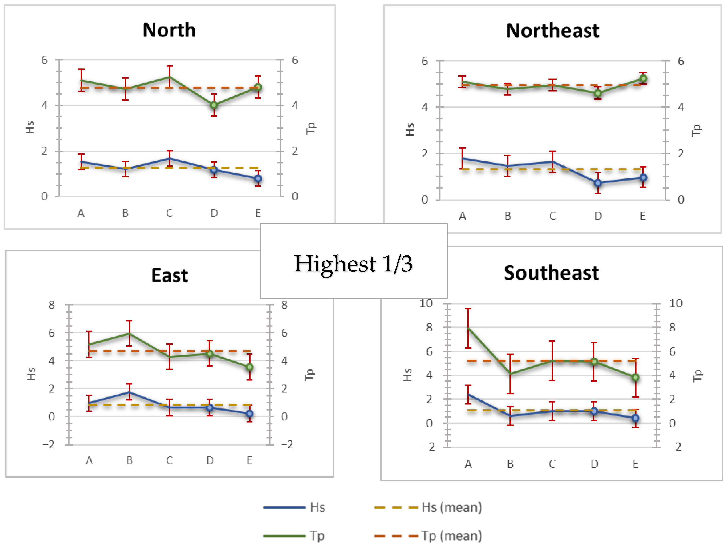
The calculated values of wave height and period, along with their mean value and standard deviation, are presented as the highest 1/3, 1/10, and 1/100 waves, for the four main directions, in

Table 6. The predicted wave height (H) and period (T) values obtained by applying the two forecasting methods (SMB and JONSWAP) to three different data sources (Skyros meteorological station, Atlas I and Atlas II), along with those results provided from the elaboration of datasets from two sources (Atlas II and Copernicus Med_wave) for the four main directions for the highest 1/3 of the waves.

Highest 1/3		N		NE		E		SE
Data Source	Method	H	Tp	H	Tp	H	Tp	H	Tp
Skyros_wind	SMB (24°)	1.77	6.02	1.62	5.17	1.15	5.66	2.87	8.61
	JONSWAP (86°)	1.28	4.17	1.96	5.05	0.81	4.72	1.92	7.29
	Average	1.53	5.10	1.79	5.11	0.98	5.19	2.39	7.95
B. Atlas I_wind	SMB (24°)	1.39	5.56	1.32	4.84	2.12	7.21	0.70	4.40
	JONSWAP (86°)	1.03	3.88	1.62	4.75	1.43	4.73	0.54	3.85
	Average	1.21	4.72	1.47	4.79	1.78	5.97	0.62	4.13
C. Copernicus Med_wind	SMB (24°)	1.95	6.22	1.48	5.02	0.80	4.71	1.21	5.80
	JONSWAP (86°)	1.41	4.30	1.80	4.92	0.54	3.87	0.77	4.63
	Average	1.68	5.26	1.64	4.97	0.67	4.29	0.99	5.22
D. Atlas II_wave	This study	1.18	4.02	0.73	4.62	0.66	4.53	1.02	5.14
E. Copernicus Med_wave	This study	0.81	4.81	0.98	5.26	0.23	3.57	0.41	3.82
Mean		1.28	4.78	1.32	4.95	0.86	4.71	1.09	5.25
Standard Deviation		0.34	0.48	0.45	0.25	0.58	0.91	0.77	1.63

,

Table 7. The predicted wave height (H) and period (T) values obtained by applying the two forecasting methods (SMB and JONSWAP) to three different data sources (Skyros meteorological station, Atlas I and Atlas II), together with those results provided from the elaboration of datasets from two sources (Atlas II and Copernicus Med_wave) for the four main directions for the highest 1/10 of the waves.

Highest 1/10		N		NE		E		SE
Data Source	Method	H	Tp	H	Tp	H	Tp	H	Tp
A. Skyros_wind	SMB (24°)	2.66	6.89	2.26	5.77	2.20	7.29	4.58	10.04
	JONSWAP (86°)	1.87	4.72	2.66	5.59	1.48	4.78	2.49	5.81
	Average	2.27	5.81	2.46	5.68	1.84	6.04	3.54	7.93
B. Atlas I_wind	SMB (24°)	2.72	6.94	2.18	5.71	2.00	7.07	3.80	9.44
	JONSWAP (86°)	1.90	4.75	2.58	5.54	1.30	5.99	2.10	5.49
	Average	2.31	5.84	2.38	5.62	1.65	6.53	2.95	7.47
C. Copernicus Med_wind	SMB (24°)	2.54	6.78	1.98	5.53	1.86	6.89	2.50	8.23
	JONSWAP (86°)	1.79	4.65	2.36	5.37	1.08	5.48	1.21	5.79
	Average	2.17	5.72	2.17	5.45	1.47	6.19	2.00	7.34
D. Atlas II_wave	This study	2.16	5.71	2.52	6.77	1.92	6.14	3.23	7.48
E. Copernicus Med_wave	This study	1.13	4.93	2.09	6.25	1.18	5.43	1.22	5.53
Mean		2.01	5.60	2.32	5.95	1.61	6.06	2.59	7.15
Standard Deviation		0.49	0.38	0.19	0.55	0.30	0.40	0.50	0.93

and

Table 8. The predicted wave height (H) and period (T) values obtained by applying the two forecasting methods (SMB and JONSWAP) to three different data sources (Skyros meteorological station, Atlas I and Atlas II), together with those results provided from the elaboration of datasets from two sources (Atlas II and Copernicus Med_wave) for the four main directions for the highest 1/100 of the waves.

Highest 1/100		N		NE		E		SE
Data Source	Method	H	Tp	H	Tp	H	Tp	H	Tp
A. Skyros_wind	SMB (24°)	4.20	8.01	2.97	6.32	3.99	8.87	7.35	11.74
	JONSWAP (86°)	2.87	5.44	3.46	6.10	2.54	5.71	3.89	6.73
	Average	3.51	6.70	4.23	7.50	3.07	7.00	4.84	8.33
B. Atlas I_wind	SMB (24°)	5.85	8.93	4.52	7.26	5.32	9.75	9.07	12.58
	JONSWAP (86°)	3.96	6.05	5.22	6.98	3.33	6.25	4.76	7.19
	Average	4.90	7.49	4.87	7.12	4.32	8.00	6.92	9.89
C. Copernicus Med_wind	SMB (24°)	3.47	7.52	2.62	6.06	3.32	8.35	3.79	9.43
	JONSWAP (86°)	2.13	4.93	3.06	5.86	3.06	9.21	1.87	5.29
	Average	2.80	6.23	2.84	5.96	3.19	8.78	2.83	7.36
D. Atlas II_wave	This study	3.20	7.73	4.59	7.73	2.71	6.30	6.91	9.89
E. Copernicus Med_wave	This study	3.75	6.98	5.02	7.99	3.62	7.08	2.82	7.31
Mean		3.64	7.03	4.11	7.00	3.33	7.11	5.04	8.76
Standard Deviation		0.79	0.60	1.01	0.90	0.67	0.62	2.04	1.28

, respectively. Furthermore, the mean values, along with their maximum and minimum values, for the five data sources (A–E), are presented in the diagrams of Figure 3, Figure 4 and Figure 5, together with their mean value and standard deviation.

Table 6 reveals that, in the case of the highest 1/3 of the waves, the SE direction consistently shows larger and more energetic waves, especially in wind-based predictions. Skyros wind data combined with SMB tends to produce the highest H and Tp values, suggesting that it is the most energetic input. Moreover, wave data sources (Atlas II and Copernicus Med_wave) yield more conservative estimates, which may reflect actual measurements rather than model extrapolations. The JONSWAP method generally gives lower wave heights and periods compared to SMB, likely due to differences in model assumptions.

The SE sector has the highest Hs and Tp values in most methods and datasets. The CEM method is used to predict the most energetic sea states. Wave datasets (Atlas II and Copernicus) tend to produce lower wave height estimates, which may be more realistic as they are based on measured values. The JONSWAP predictions are usually lower than the CEM predictions, both in Hs and Tp, for all directions and wind datasets. The SE and NE directions show the most variation in both Hs and Tp, suggesting that the waves in these areas are more unstable.

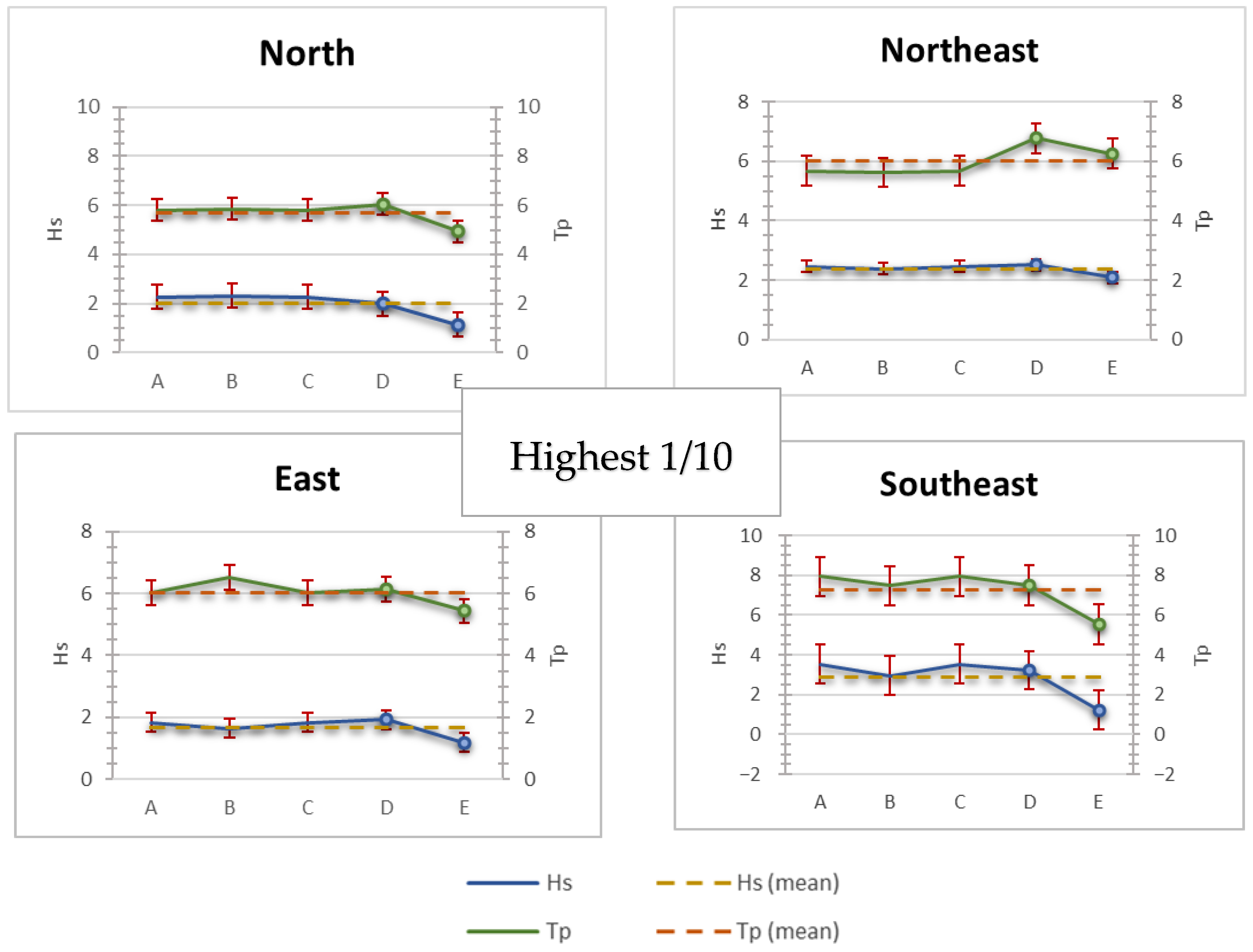
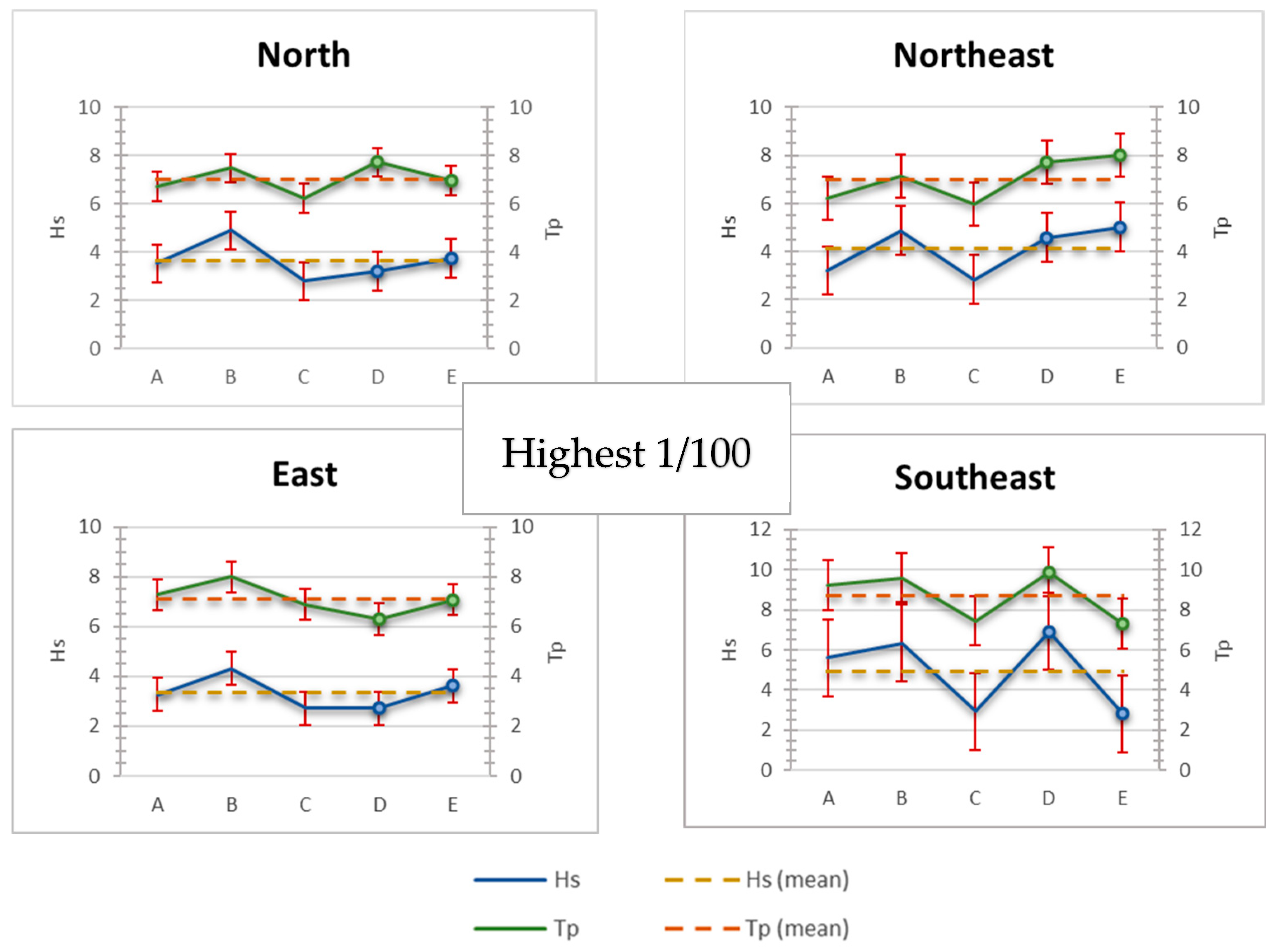
Finally, an analysis of the highest 1/100 of the waves (see Table 8) reveals that the SE direction is the most energetic, both in Hs and Tp; this is due to the fact that the SE direction coincides with the longest fetch distance. It is also noteworthy that the forecasts are most extreme when using the CEM method and the Atlas I wind dataset. Conversely, the lowest values are observed when employing the JONSWAP method with the Copernicus dataset.

5. Discussion

The discussion of the results in relation to the prediction of the highest 1/3, 1/10, and 1/100 of the waves focuses on the comparison of the following: (i) the application of two methods (SMB and JONSWAP) to predict wave characteristics using wind datasets from three different sources; (ii) the wave characteristics calculated from the ATLAS II and the Copernicus Med_wave datasets; (iii) the predicted wave characteristics (mean values) from wind and wave datasets; and (iv) the conclusive estimates of wave height and period derived from the applied methods and datasets, relatively to individual prognostic estimate.

5.1. Comparing the Results of the Forecasting Methods (Wind Data)

In the case of wind data from three different sources, the SMB method based on an effective fetch calculated over a 24° arc yields higher values for both wave height and period compared to the JONSWAP method, which uses an effective fetch derived from a 90° arc (see

Table 9. The percentage differences (%) of wave characteristics (H, Tp) between the two prediction methods (SMB vs. JONSWAP) for the three-wind datasets, and for the highest 1/3, 1/10, and 1/100 of the waves.

Highest 1/3	N		NE		E		SE
	H	Tp	H	Tp	H	Tp	H	Tp
Skyros	27.6	31.0	17.3	2.3	29.6	16.6	33.1	15.3
Atlas I	25.9	30.2	18.5	1.9	32.5	34.4	22.6	12.5
Copernicus	27.7	23.2	17.3	2.0	32.5	17.8	33.9	20.2
Highest 1/100	N		NE		E		SE
	H	Tp	H	Tp	H	Tp	H	Tp
Skyros	30.0	31.5	15.0	3.1	32.7	34.4	47.6	42.3
Atlas I	30.1	31.6	15.5	3.0	35.0	15.3	44.7	41.8
Copernicus	27.7	19.0	19.0	2.9	39.8	20.5	40.0	21.6
Highest 1/10	N		NE		E		SE
	H	Tp	H	Tp	H	Tp	H	Tp
Skyros	31.7	32.1	14.2	3.5	36.3	35.6	47.1	42.7
Atlas I	32.3	32.2	24.9	3.9	37.6	35.9	47.5	42.8
Copernicus	38.6	34.4	17.0	3.0	35.5	35.3	44.8	42.7

). The differences in height are in the order of 17.3–33.9% for the highest 1/3, 15–47.6% for the highest 1/10, and 14.2–47.5% for the highest 1/100 of the waves. The corresponding ranges of wave period values are 1.9–31% for the highest 1/3, 2.9–42.5% for the highest 1/10, and 3–42.8% for the highest 1/100 of the waves. It has been established that the smallest disparities (in cases where H < 25% and T < 3%) are observable in the NE direction, which concomitantly exhibits the most substantial disparity in terms of wave fetch distance. Conversely, the SE direction exhibits the largest values (for H > 33%, and for T > 12%). These variations can be attributed to differences in wind data sources (i.e., geographical position and/or spatial coverage, time step, and period of wind measurements), as well as to the prediction methods employed, as described in the methodology (Section 3.2).

5.2. Comparing the Results of Processing Wave Metadata (ATLAS II, Copernicus Med_wave)

A notable disparity is evident in the wave values derived from the elaboration of the ATLAS II dataset and those derived from the Copernicus database. The differences in wave height and period values, expressed as percentages, are generally in the order of 9–65% and 9.5–26.1%, respectively (

Table 10. The percentage differences (%) for the values of H and T, as predicted by the ATLAS II and Copernicus Med_wave datasets.

	N		NE		E		SE
	H	Tp	H	Tp	H	Tp	H	Tp
1/3	31.3	20.8	25.5	12.2	65.0	21.2	59.8	25.7
1/10	47.7	13.7	16.3	7.7	38.5	11.6	62.2	26.1
1/100	9.3	9.7	8.6	3.2	25.1	11.0	59.2	26.1

). Furthermore, the differences in wave height and period for the highest 1/3 and the highest 1/10 of the waves are small (<10%), but significantly higher (2–3 times) to those referred to the highest 1/100 waves for all directions, with the exception of the SE, where they are similar. The variations in wave height and period can be attributed to the different types and origins of the datasets (i.e., covering different geographical areas and time periods), as described in Section 3.1, and to the presence of a large number of islands (i.e., influencing effective fetch distances).

5.3. Comparing the Results (H, T) Based on Wind and Wave Databases

In order to facilitate a comparison between the H and Tp values, their average values for the highest 1/3, 1/10, and 1/100 of the waves, derived from the three wind datasets (WD), the Atlas II wave dataset (WA), and the Copernicus MED_wave (CW), have been cross-compared. The resulting differences, expressed as percentages, are presented in

Table 11. The predicted average height (H) and peak period (T) values for the highest 1/3, 10/100, and 1/100 of the waves for the three wind databases (WD), the ATLAS II (WA) and Copernicus Med_wind (CW) and their differences expressed as percentages for the N, NE, E, and SE directions.

Highest 1/3	N		NE		E		SE
	H	Tp	H	Tp	H	Tp	H	Tp
WD	1.47	5.03	1.63	4.96	1.14	5.15	1.33	5.77
WA	1.18	4.02	0.73	4.63	0.66	4.53	1.02	5.14
WC	0.81	4.81	0.98	5.26	0.23	3.57	0.41	3.82
WD-WA (%)	19.91	20.03	55.31	6.59	42.27	12.04	23.50	10.87
WD-WC (%)	45.02	4.31	40.00	−6.12	79.88	30.68	69.25	33.76
WA-WC (%)	31.12	19.65	34.25	−13.85	65.5	21.19	59.78	25.70
Highest 1/10	N		NE		E		SE
	H	Tp	H	Tp	H	Tp	H	Tp
WD	2.84	6.23	2.57	5.16	2.37	6.71	3.78	7.36
WA	4.04	8.16	2.52	6.77	1.92	6.14	3.23	7.48
WC	1.13	4.93	2.09	6.25	1.18	5.43	1.22	5.53
WD-WA (%)	−42.09	−30.98	2.07	−31.12	19.10	8.45	14.47	−1.58
WD-WC (%)	60.26	20.87	18.78	−21.05	50.28	19.04	67.70	24.90
WA-WC (%)	43.2	18.51	17.06	7.68	38.63	11.60	62.19	26.06
Highest 1/100	N		NE		E		SE
	H	Tp	H	Tp	H	Tp	H	Tp
WD	3.74	6.81	3.98	6.86	3.53	7.93	4.90	8.56
WA	3.20	7.73	4.59	7.73	2.71	6.30	6.91	9.89
WC	3.75	6.98	5.02	7.99	3.62	7.08	2.82	7.31
WD-WA (%)	14.36	−13.57	−15.33	−12.68	23.16	20.52	−41.02	−15.58
WD-WC (%)	−0.36	−2.55	−26.13	−16.47	−2.65	10.68	42.45	14.57
WA-WC (%)	−17.19	9.70	−9.37	−3.36	−33.58	−12.38	59.19	26.09

.

In the case of the highest 1/3 waves, the ATLAS II (WA) values of Hs and Tp are lower than the mean values from the three wind datasets (WD), by 19.9–55.4% for Hs and 6.5–20% for Tp. In comparison to the Copernicus MED_wave (CW), WC values are characterized by either larger or smaller values, depending on the direction. The largest disparities (>42%) are associated with the SE and E directions, while the N and NE directions demonstrate comparatively smaller differences (<23.5%).

A similar overall pattern is observed in the case of the highest 1/10 of the waves, although the magnitude of the differences appears to be somewhat elevated, with the most pronounced variation observed between the WD and WA datasets. Thus, the highest 1/10 waves show percentage differences of 2–42% for H(1/10) and 1.5–31% for Tp(1/10). With respect to wave direction, the WA values for the N direction demonstrate the most significant variations (up to 42% for H(1/10) and 31% for Tp(1/10), while very small variations in height are exhibited by the NE direction (approximately 2.5%), although the Tp (1/10) value is analogous to those of the N direction. It is evident that the E and SE directions exhibit minimal disparities in both H(1/10) and T(1/10), in comparison to the other directions. The values from the Copernicus MED_wave dataset (CW) demonstrate a greater deviation in wave height compared to WD for wave height (H(1/10) = 18.8–67.7%), while in terms of period Tp(1/10), they are comparable (19–25%) for the N and NE directions but significantly larger (>60%) for the E and SE directions.

It is evident that the highest 1/100 waves exhibit significantly smaller differences of less than 27% for wave height H(1/100) and less than 21% for peak period Tp(1/100) (in absolute values) when compared to wind data (WD). An exception is observed in the SE direction, where wave height differences range between 40% and 60%.

The variability in offshore wave characteristics described above can be attributed to the diverse sources of the original wind and wave data, in terms of space coverage and time span, the different methodologies applied, and the substantial differences in fetch distances between the examined directions. Nevertheless, all the prognostic values are within the anticipated range for the Mediterranean Sea, a topic which is discussed in greater detail in the subsequent section.

5.4. Overall Estimate of Height and Period

As illustrated in

Table 12. Mean values and Standard Deviation of wave height (H) and period (Tp) for the wind and wave datasets, and for the highest 1/3, 1/10, and 1/100 of the waves.

Highest 1/3		N		NE		E		SE
		H	Tp	H	Tp	H	Tp	H	Tp
Wind datasets	Mean	2.01	5.53	2.26	5.59	1.63	5.62	2.45	7.25
	STDV	0.71	0.62	0.47	0.41	0.96	1.31	1.37	1.93
Wave datasets	Mean	0.98	4.40	0.83	4.90	0.45	4.05	0.70	4.46
	STDV	0.27	0.54	0.14	0.39	0.30	0.68	0.45	0.96
All datasets	Mean	1.60	5.08	1.68	5.32	1.16	4.99	1.75	6.13
	STDV	0.76	0.80	0.85	0.52	0.95	1.31	1.38	2.10
Highest 1/10		N		NE		E		SE
		H	Tp	H	Tp	H	Tp	H	Tp
Wind datasets	Mean	2.95	6.30	2.62	5.60	2.30	6.64	3.51	7.89
	STDV	0.61	0.44	0.53	0.80	1.25	0.83	1.64	0.98
Wave datasets	Mean	1.56	5.49	1.83	5.85	1.44	5.54	2.18	6.39
	STDV	0.61	0.79	0.98	1.30	0.68	0.85	1.48	1.54
All datasets	Mean	2.40	5.98	2.30	5.70	1.96	6.20	2.98	7.29
	STDV	0.93	0.67	0.76	0.87	1.06	0.94	1.56	1.33
Highest 1/100		N		NE		E		SE
		H	Tp	H	Tp	H	Tp	H	Tp
Wind datasets	Mean	3.62	6.75	3.50	6.50	3.46	7.94	4.98	9.06
	STDV	0.81	0.50	0.60	0.36	0.65	0.36	1.58	0.44
Wave datasets	Mean	3.48	7.36	4.17	7.36	2.96	6.56	4.07	7.77
	STDV	0.39	0.53	0.59	0.53	0.35	0.37	1.91	0.80
All datasets	Mean	3.56	6.99	3.77	6.84	3.26	7.39	4.62	8.54
	STDV	0.61	0.55	0.63	0.60	0.56	0.82	1.55	0.87

, the mean and standard deviation values of wave height (H) and period (T) for the highest 1/3, 1/10, and 1/100 waves have been deduced from the mean values of the following: (i) the three wind datasets, the (ii) the two wave datasets, and (iii) the combination of the five datasets.

It is evident that the mean values derived from the wind datasets are generally larger than those obtained from the two wave datasets. However, the mean values derived from the five datasets reveal that they fall between these two groups.

This overestimation of wind-based prognostic methods in the case of the Mediterranean Sea can be explained by the fact that wind hindcasting methods are usually based on fully developed seas, while wave datasets are based on metadata originating from either observed actual wave conditions or in situ wave measurements. Consequently, the mean values derived from the five datasets could be regarded as more representative, as they compensate for the variations inherent in the different methods and datasets. The aforementioned values are consistent with the maximum offshore values anticipated for the Mediterranean Sea (i.e., Hs (max) ≤ 6 m and Ts (max) < 12 s), as asserted by Cavaleri et al. [8] and documented in the case of the NE Mediterranean [8], the east coast of Adriatic [30], and the SE Mediterranean [31]. However, it should be noted that extreme waves, defined as the largest waves occurring within 12 h per year, were not isolated in this study.

In instances where there is an absence of suitable offshore wave data that spans a sufficient time period, the prognostic equations presented in this study appear to yield reasonable results. These equations may be employed for a variety of purposes, including offshore installations and the mitigation of coastal erosion. In instances where wind data are the sole available metric, it is recommended that wave characteristics be estimated through the application of both the SPM [29] and JONSWAP [27] approaches, in conjunction with the requisite fetch distances calculated employing an arc of 24 or 84 degrees. Subsequently, the mean values are to be derived. The same approach is proposed in the case of wave data (or metadata) being available, i.e., the estimation of the wave characteristics for each dataset separately, and thereafter, to calculate the mean values. In instances where both wind and wave data are available, the method outlined in this study can be utilised.

6. Synopsis and Conclusions

The two approaches for calculating the effective fetch distances yield values that differ substantially, particularly in the E and SE directions, which are the directions where the effective fetch is most influenced by the presence of islands.

In general, the mean values from the three wind datasets provide higher values for both wave height and peak period in comparison to the mean values of the wave datasets. In addition, the prognostic equations of the SMB method, when employed in conjunction with effective fetch distances of 24 degrees, yield higher wave heights and peak periods than the JONSWAP method with an effective fetch of 84 degrees, as evidenced by the analysis of three wind datasets.

Beyond the methodology employed, variations in the estimated values from the three wind datasets and the two wave datasets are attributed to differences in the methodology of assimilating the raw data, as well as their spatial and temporal coverage by each dataset.

The proposed methodology for calculating wave heights and periods for the highest 1/10 and 1/100 of the waves from the three wind datasets and the two wave datasets appears to yield reasonable outcomes when compared to the corresponding significant (highest 1/3) wave heights and periods.

The wave characteristics provided as mean values from the three wind datasets are larger than the mean values estimated from the two wave datasets. Ultimately, the mean values of wave height and period calculated from the five available datasets, considering their standard deviation, appear to be more representative than the values calculated separately from each dataset.

References

- Haslett, S. Coastal Systems, 2nd ed.; Routledge: London, UK, 2009. [Google Scholar] [CrossRef]
- Elkut, A.E.; Taha, M.T.; Zed, A.B.E.A.; Eid, F.M.; Abdallah, A.M. Wind-wave hindcast using modified ECMWF ERA-Interim wind field in the Mediterranean Sea. Estuar. Coast. Shelf Sci. 2021, 252, 107267. [Google Scholar] [CrossRef]
- Caires, S.; Sterl, A.; Bidlot, J.R.; Graham, N.; Swail, V. Intercomparison of different wind–wave reanalyses. J. Clim. 2004, 17, 1893–1913. [Google Scholar] [CrossRef]
- Cavaleri, L.; Bertotti, L.; Lionello, P. Wind wave cast in the Mediterranean Sea. J. Geophys. Res. 1991 Ocean. 1991, 96, 10739–10764. [Google Scholar] [CrossRef]
- Lionello, P.; Sanna, A. Mediterranean wave climate variability and its links with NAO and Indian Monsoon. Clim. Dyn. 2005, 25, 611–623. [Google Scholar] [CrossRef]
- Stefanakos, C.N.; Athanassoulis, G.A.; Cavaleri, L.; Bertotti, L.; Lefèvre, J.M. Wind and wave climatology of the Mediterranean Sea. Part I: Wind statistics. In Proceedings of the ISOPE International Ocean and Polar Engineering Conference, Toulon, France, 23–28 May 2004; ISOPE: Mountain View, CA, USA, 2004; pp. 187–196. [Google Scholar]
- Barbariol, F.; Davison, S.; Falcieri, F.M.; Ferretti, R.; Ricchi, A.; Sclavo, M.; Benetazzo, A. Wind waves in the Mediterranean Sea: An ERA5 reanalysis wind-based climatology. Front. Mar. Sci. 2021, 8, 760614. [Google Scholar] [CrossRef]
- Ardhuin, F.; Bertotti, L.; Bidlot, J.R.; Cavaleri, L.; Filipetto, V.; Lefevre, J.M.; Wittmann, P. Comparison of wind and wave measurements and models in the Western Mediterranean Sea. Ocean. Eng. 2007, 34, 526–541. [Google Scholar] [CrossRef]
- Bolaños-Sanchez, R.; Sanchez-Arcilla, A.; Cateura, J. Evaluation of two atmospheric models for wind–wave modelling in the NW Mediterranean. J. Mar. Syst. 2007, 65, 336–353. [Google Scholar] [CrossRef]
- Saviano, S.; Cianelli, D.; Zambianchi, E.; Conversano, F.; Uttieri, M. An integrated reconstruction of the multiannual wave pattern in the Gulf of Naples (South-Eastern Tyrrhenian Sea, Western Mediterranean Sea). J. Mar. Sci. Eng. 2020, 8, 372. [Google Scholar] [CrossRef]
- Pomaro, A.; Cavaleri, L.; Lionello, P. Climatology and trends of the Adriatic Sea wind waves: Analysis of a 37-year long instrumental data set. Int. J. Climatol. 2017, 37, 4237–4250. [Google Scholar] [CrossRef]
- Katalinić, M.; Ćorak, M.; Parunov, J. Analysis of wave heights and wind speeds in the Adriatic Sea. Marit. Technol. Eng. 2014, 1, 1389–1394. [Google Scholar]
- Nafaa, M.G.; Fanos, A.M.; Elganainy, M.A. Characteristics of waves off the Mediterranean coast of Egypt. J. Coast. Res. 1991, 7, 665–676. [Google Scholar]
- Frihy, O.E.; Deabes, E.A.; El Gindy, A.A. Wave climate and nearshore processes on the Mediterranean coast of Egypt. J. Coast. Res. 2010, 26, 103–112. [Google Scholar] [CrossRef]
- Zed, A.A.A.; Kansoh, R.M.; Iskander, M.M.; Elkholy, M. Wind and wave climate southeastern of the Mediterranean Sea based on a high-resolution SWAN model. Dyn. Atmos. Ocean. 2022, 99, 101311. [Google Scholar] [CrossRef]
- Soukissian, T.H.; Prospathopoulos, A.M.; Diamanti, C. Wind and wave data analysis for the Aegean Sea-preliminary results. Glob. Atmos. Ocean. Syst. 2002, 8, 163–189. [Google Scholar] [CrossRef]
- Karditsa, A.; Poulos, S.E. Sedimentological investigations in a river-influenced tideless coastal embayment: The case of inner continental shelf of the NE Aegean Sea. Cont. Shelf Res. 2013, 55, 86–96. [Google Scholar] [CrossRef]
- Poulos, S.E.; Ghionis, G.; Verykiou, E.; Roussakis, G.; Sakellariou, D.; Karditsa, A.; Georgiou, P. Hydrodynamic, neotectonic and climatic control of the evolution of a barrier beach in the microtidal environment of the NE Ionian Sea (eastern Mediterranean). Geo-Mar. Lett. 2015, 35, 37–52. [Google Scholar] [CrossRef]
- Bourma, E.; Perivoliotis, L.; Petihakis, G.; Korres, G.; Frangoulis, C.; Ballas, D.; Zervakis, V.; Tragou, E.; Katsafados, P.; Spyrou, C.; et al. The hellenic marine observing, forecasting and technology system—An integrated infrastructure for marine research. J. Mar. Sci. Eng. 2022, 10, 329. [Google Scholar] [CrossRef]
- Poulos, S.E.; Drakopoulos, P.; Collins, M.B. Seasonal variability in the oceanographic conditions in the Aegean Sea (eastern Mediterranean): An overview. J. Mar. Syst. 1997, 13, 225–244. [Google Scholar] [CrossRef]
- Hasselmann, D.E.; Dunckel, M.; Ewing, J.A. Directional wave spectra observed during JONSWAP 1973. J. Phys. Oceanogr. 1980, 10, 1264–1280. [Google Scholar] [CrossRef]
- USACE (United States Army Corps of Engineers). Coastal Engineering Manual; US Army Corps of Engineers: Washington, DC, USA, 2002. [Google Scholar]
- Athanasoulis, G.; Skarsoulis, E. Wind and Wave Atlas of the Northeast Mediterranean Sea; National Technical University of Athens: Athens, Greece, 1992. [Google Scholar]
- Soukissian, T.; Hatzinaki, M.; Korres, G.; Papadopoulos, A.; Kallos, G.; Anadranistakis, E. Wind and Wave Atlas of the Hellenic Seas; HCMR: Anavyssos, Greece, 2007. [Google Scholar]
- CEM. Coastal Engineering Manual. 1984. Available online: https://www.publications.usace.army.mil/USACE-Publications/Engineer-Manuals/u43544q/636F617374616C20656E67696E656572696E67206D616E75616C/ (accessed on 6 May 2023).
- Smith, J.M. Wind-Wave Generation on Restricted Fetches; Coastal Engineering Research Center: Vicksburg, MS, USA, 1991; p. 50. [Google Scholar]
- Coastal Engineering Research Center, Shore Protection Manual, 4th ed.; U.S. Government Printing: Washington, DC, USA, 1984.
- Bretschneider, C.L. The Ash Wednesday East Coast Storm, March 5–8, 1962, A Hindcast of Events, Causes, and Effects. In Coastal Engineering 1964; ASCE: Reston, VA, USA, 1964; pp. 617–659. [Google Scholar]
- Goda, Y. Random Seas and Design of Maritime Structures; World Scientific: Singapore, 2000. [Google Scholar]
- Kalinić, H.; Mihanović, H.; Cosoli, S.; Tudor, M.; Vilibić, I. Predicting ocean surface currents using numerical weather prediction model and Kohonen neural network: A northern Adriatic study. Neural Comput. Appl. 2017, 28, 611–620. [Google Scholar] [CrossRef]
- Frihy, O.; Mohamed, S.; Abdalla, D.; El-Hattab, M. Assessment of natural coastal hazards at Alexandria/Nile Delta interface, Egypt. Environ. Earth Sci. 2021, 80, 1–15. [Google Scholar] [CrossRef]
Figure 1.
The testing offshore area (Central Aegean Sea) for the various methods of calculating open sea wave characteristics approaching the east coast of Evia (port of Kymi).
Figure 2.
The arcs of 84 and 24 degrees for calculating the effective fetch distance for offshore waves approaching the Kymi coast from the N, NE, E, and SE geographical directions.
Figure 3.
The average, maximum, and minimum values of the highest 1/3 waves for the four main geographical directions, based on the results presented in