

Integrating Remote Sensing and Machine Learning for Dynamic Monitoring of Eutrophication in River Systems: A Case Study of Barato River, Japan

 ,
,  , ,
, , 
Abstract
1. Introduction
2. Materials and Methods
2.1. Study Area
2.2. Datasets
2.2.1. Satellite Data
2.2.2. In-Situ Data
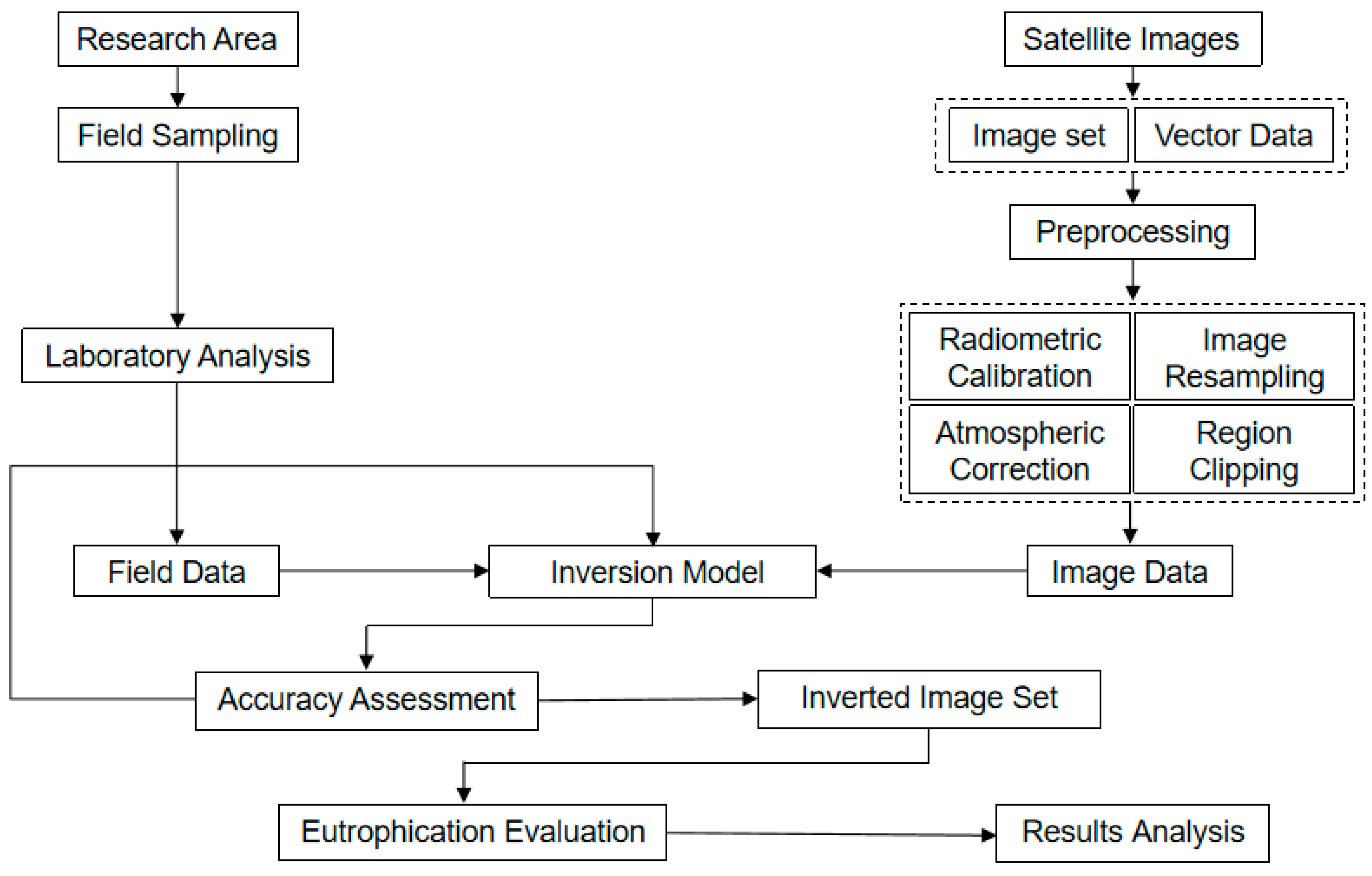
2.3. Methods
2.3.1. Image Processing and Preprocessing
2.3.2. Inversion of Eutrophication Parameter Concentrations Using Empirical Algorithms
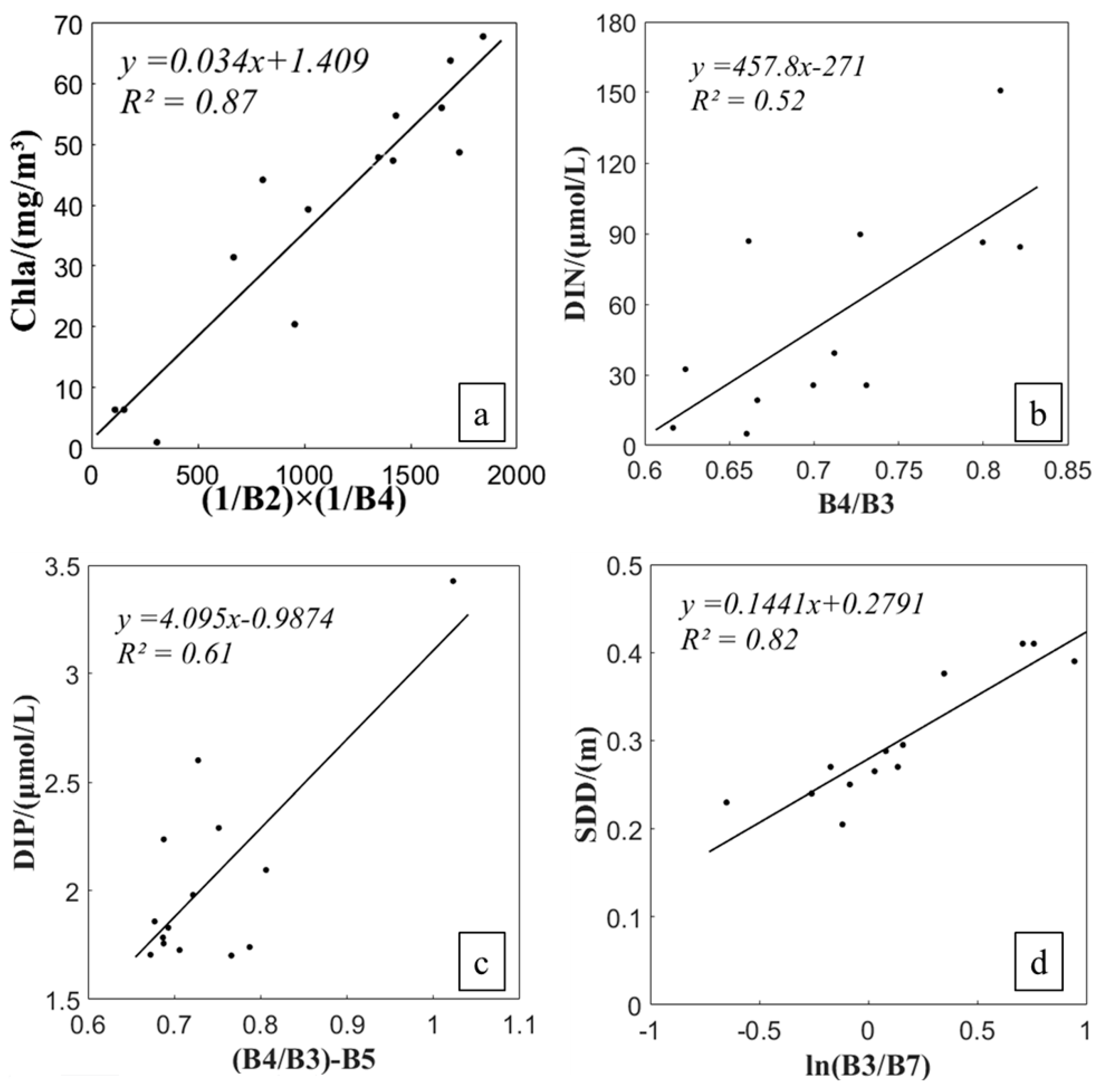
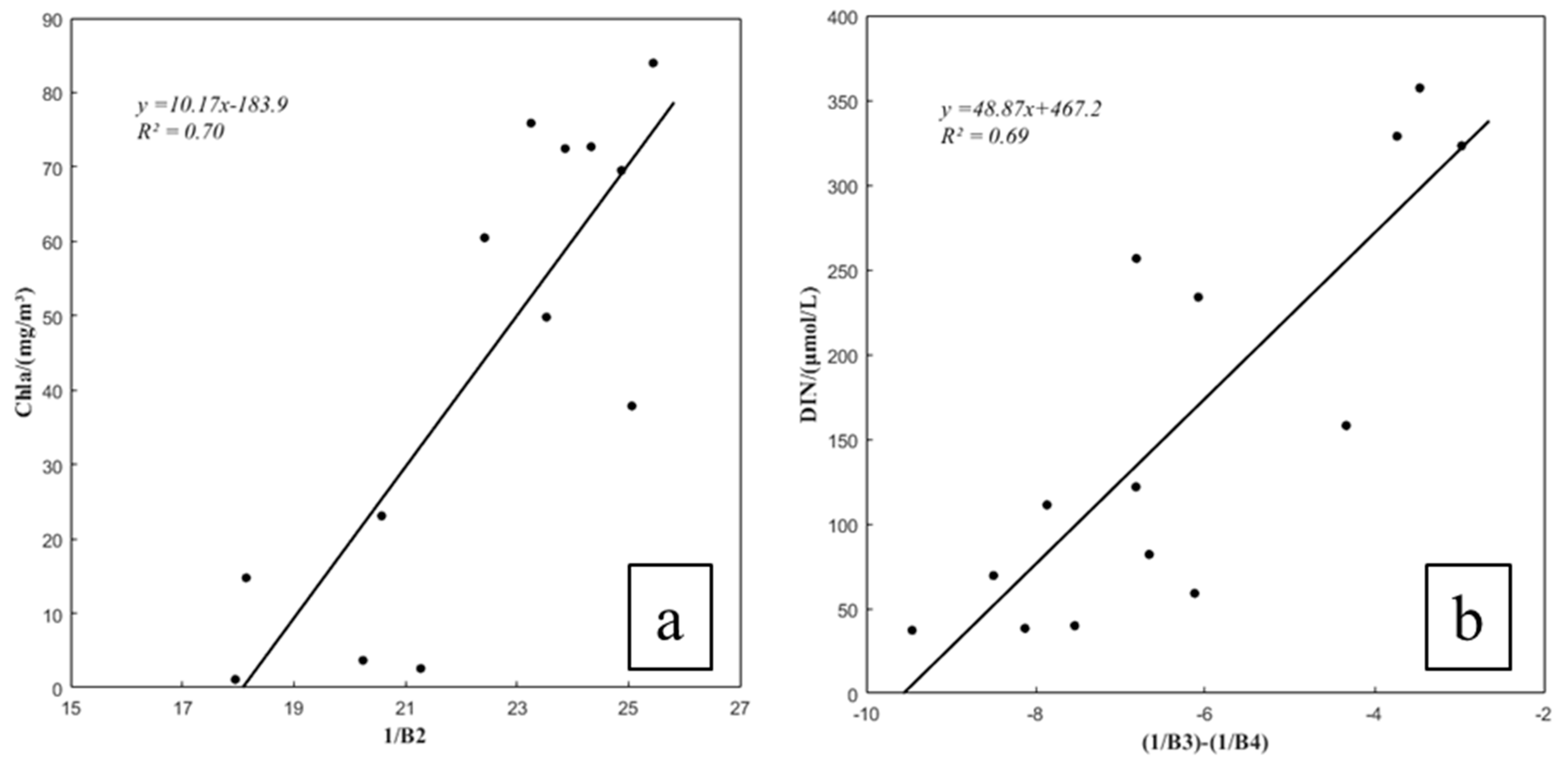
Correlation Analysis
Inversion Modeling Based on Empirical Algorithms
- (a)
- Accuracy assessment
- (b)
- Model optimization
- Staged seasonal modeling
- (c)
- Enhancing inversion accuracy with machine learning
- Accuracy assessment
2.3.3. Eutrophication Assessment Framework
Single-Factor Index (Pi) Method
Trophic State Index Modified (TSIM) Method
3. Results and Discussion
3.1. Inversion of Eutrophication Parameter Concentrations Using Empirical Algorithms
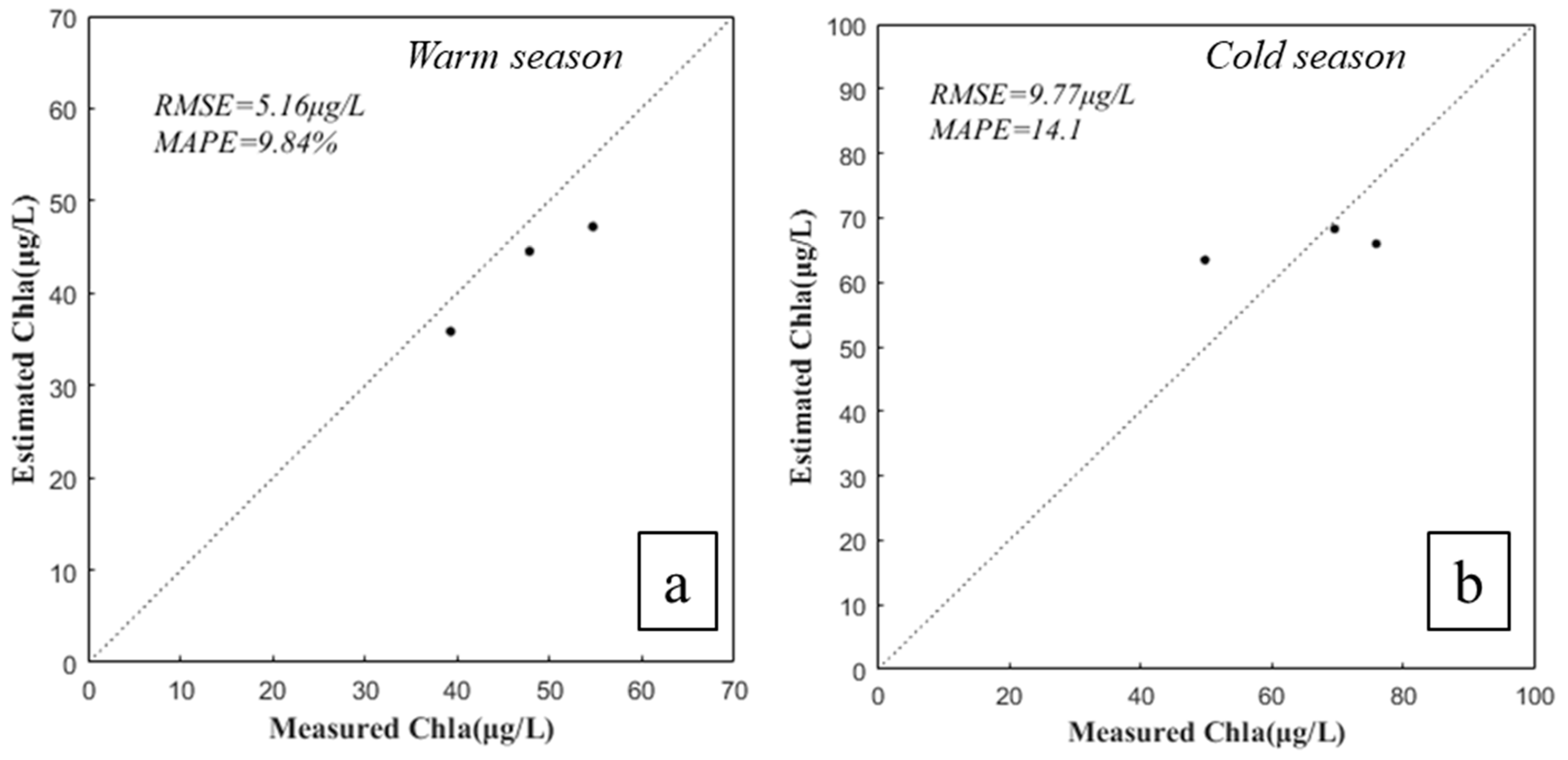
3.1.1. Accuracy Assessment
3.1.2. Back Propagation (BP) Neural Network
3.2. Temporal Dynamics of Water Quality Parameters
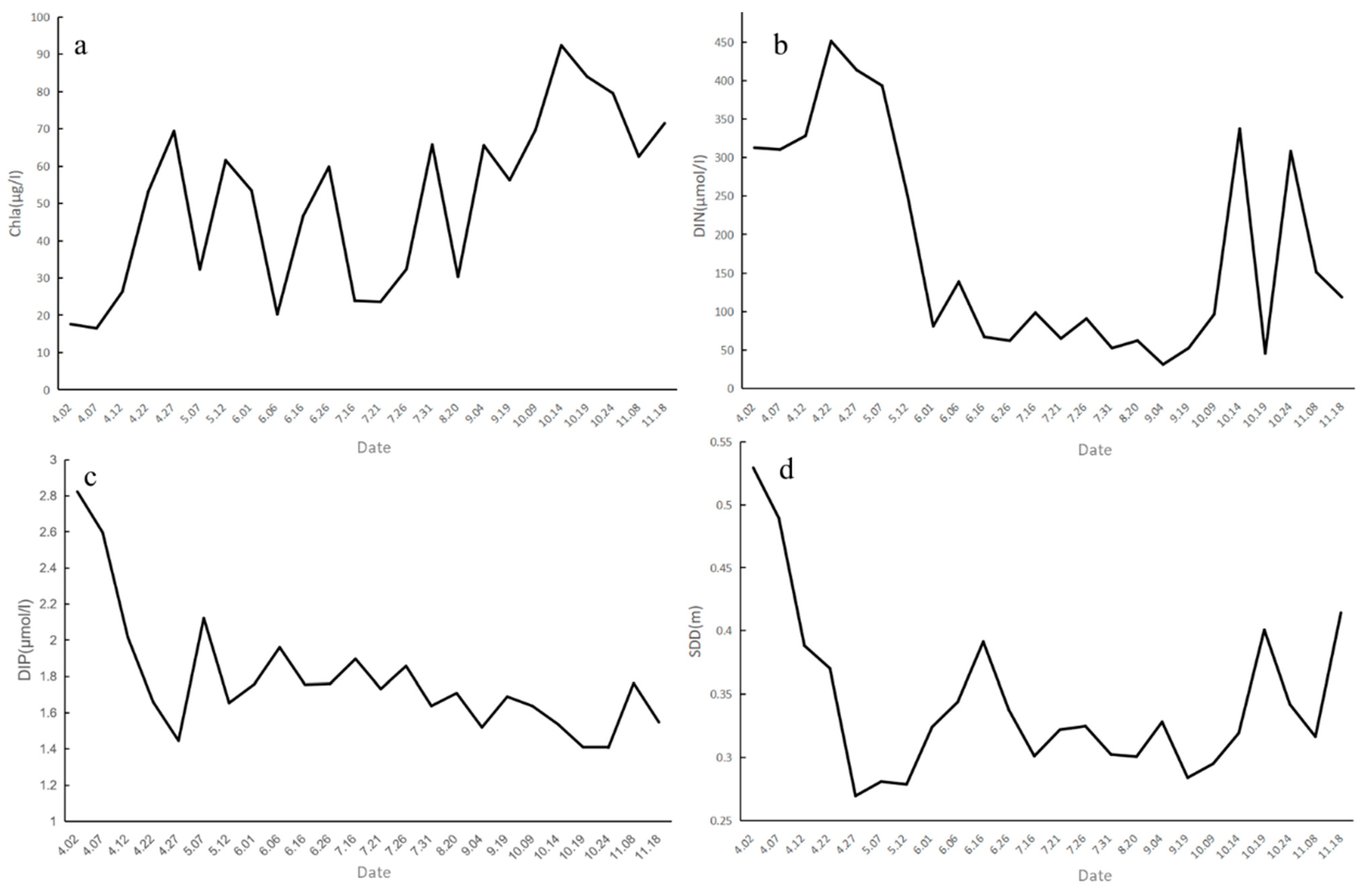
3.2.1. Dynamic Monitoring in 2021
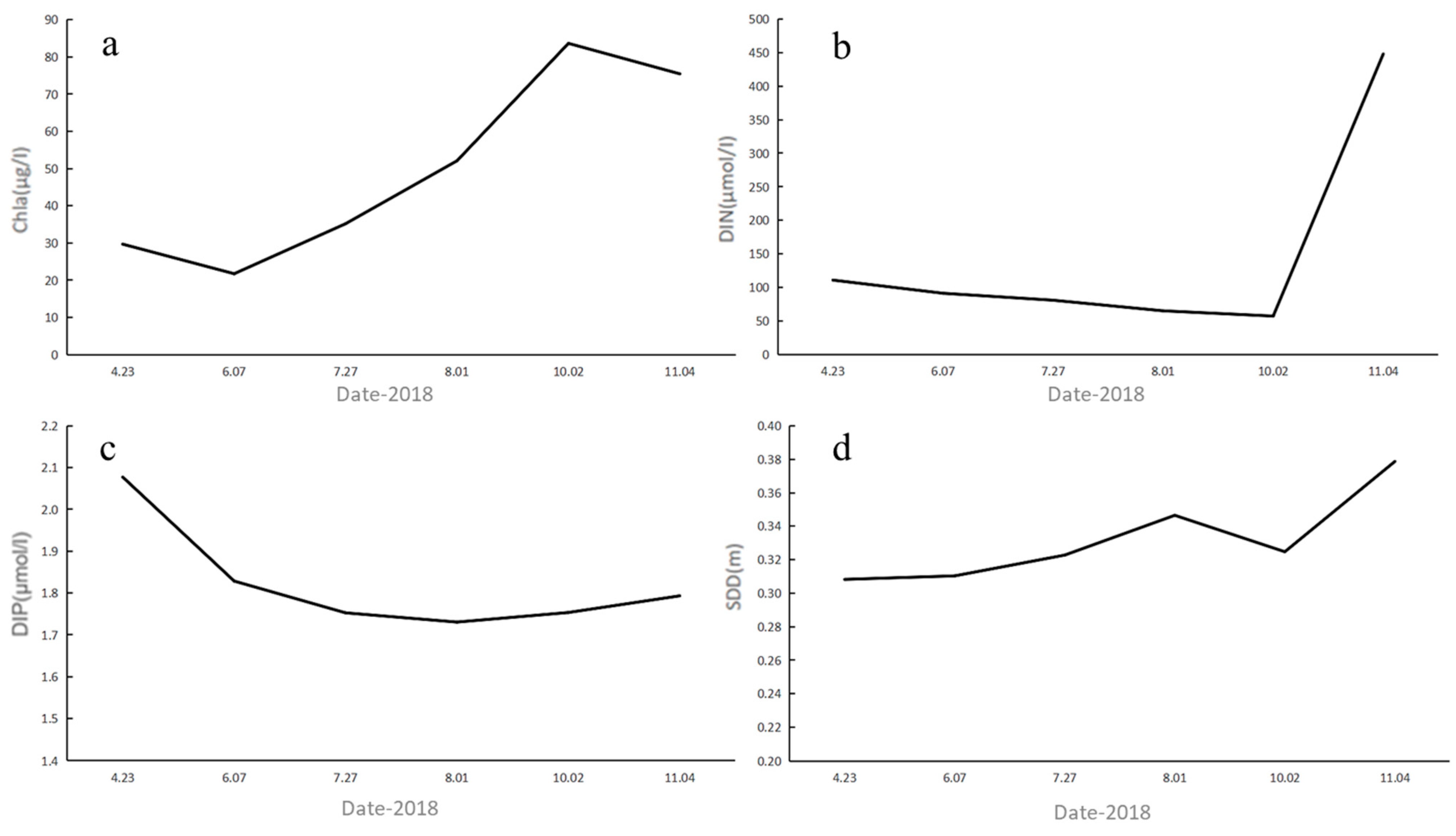
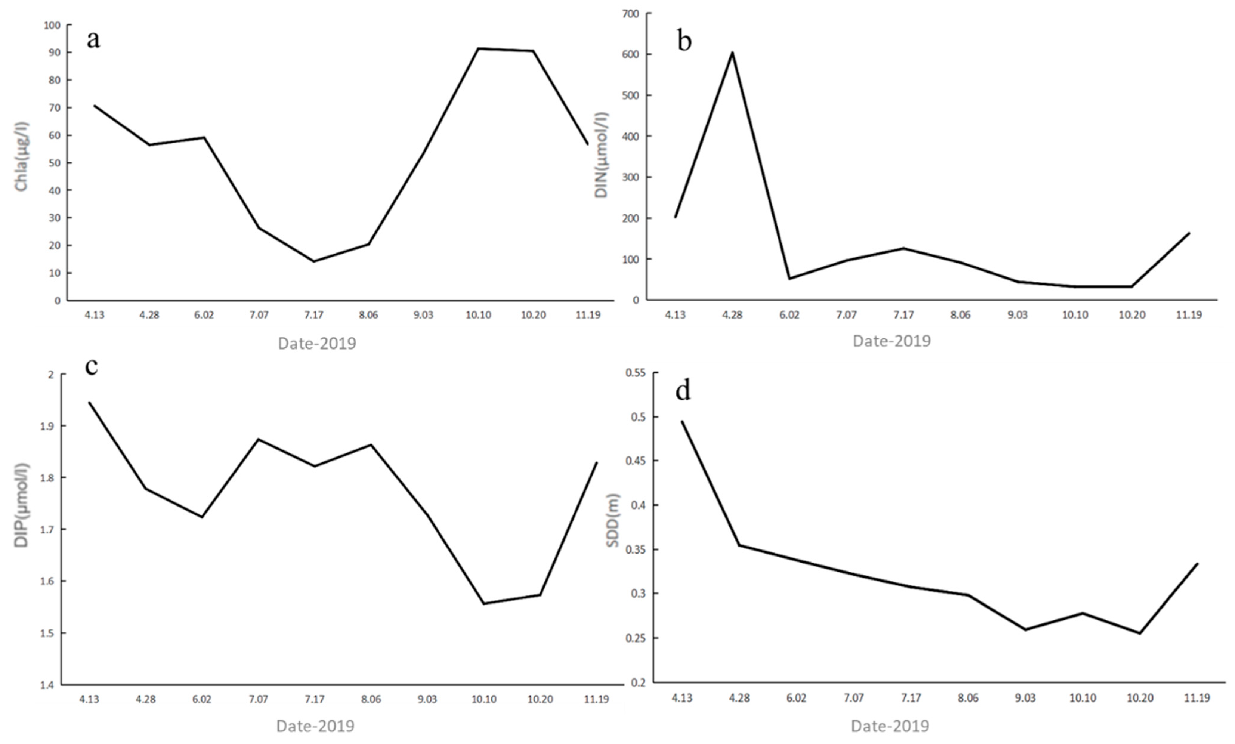
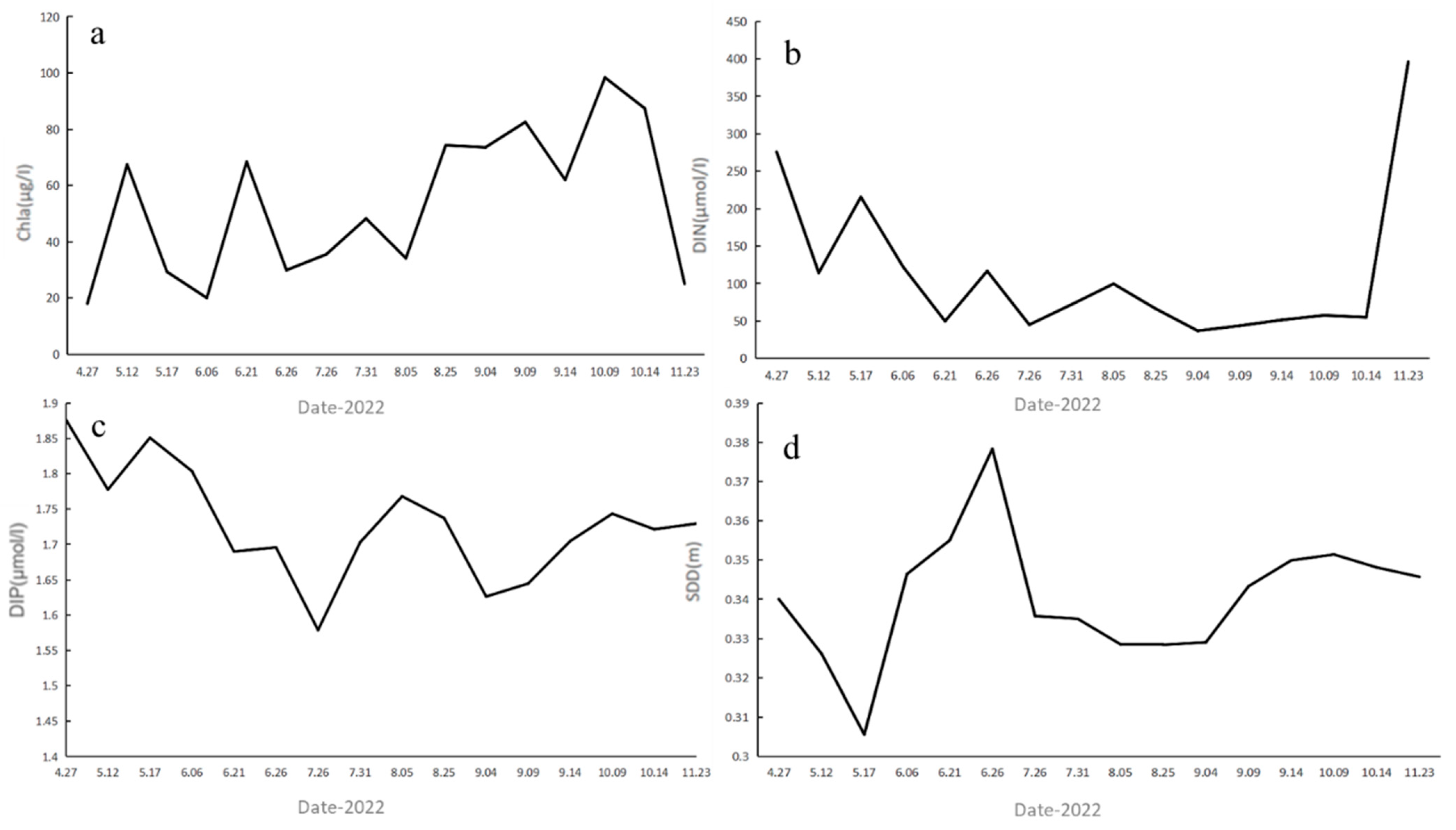
3.2.2. Multi-Year Monitoring of Eutrophication (2018–2022)
3.3. Evaluation of Eutrophication Status
3.4. Trends and Implications
4. Conclusions
Author Contributions
Funding
Data Availability Statement
Acknowledgments
Conflicts of Interest
References
- Guo, Z.; Boeing, W.J.; Borgomeo, E.; Xu, Y.; Weng, Y. Linking reservoir ecosystems research to the sustainable development goals. Sci. Total Environ. 2021, 781, 146769. [Google Scholar] [CrossRef] [PubMed]
- Primost, J.E.; Peluso, L.; Sasal, M.C.; Bonetto, C.A. Nutrient dynamics in the Paraná River Delta: Relationship to the hydrologic regime and the floodplain wetlands. Limnologica 2022, 94, 125970. [Google Scholar] [CrossRef]
- Sitote, Y.M.; Gebremedhine, M.G. Comprehensive Review of Eutrophication in Freshwater Ecosystems: Causes, Effects, Assessment, and Management Strategies. Preprints 2024. [Google Scholar] [CrossRef]
- Bănăduc, D.; Simić, V.; Cianfaglione, K.; Barinova, S.; Afanasyev, S.; Öktener, A.; McCall, G.; Simić, S.; Curtean-Bănăduc, A. Freshwater as a sustainable resource and generator of secondary resources in the 21st century: Stressors, threats, risks, management and protection strategies, and conservation approaches. Int. J. Environ. Res. Public Health 2022, 19, 16570. [Google Scholar] [CrossRef]
- Costa, D.; Sutter, C.; Shepherd, A.; Jarvie, H.; Wilson, H.; Elliott, J.; Liu, J.; Macrae, M. Impact of climate change on catchment nutrient dynamics: Insights from around the world. Environ. Rev. 2022, 31, 4–25. [Google Scholar] [CrossRef]
- Tiwari, A.K.; Pal, D.B. Nutrients contamination and eutrophication in the river ecosystem. In Ecological Significance of River Ecosystems; Elsevier: Amsterdam, The Netherlands, 2022; pp. 203–216. [Google Scholar]
- Kennedy, R.H.; Walker, W.W. Reservoir nutrient dynamics. In Reservoir Limnology: Ecological Perspectives; Wiley: New York, NY, USA, 1990; pp. 109–131. [Google Scholar]
- Brett, M.T.; Benjamin, M.M. A review and reassessment of lake phosphorus retention and the nutrient loading concept. Freshw. Biol. 2008, 53, 194–211. [Google Scholar] [CrossRef]
- Hilton, J.; O’Hare, M.; Bowes, M.J.; Jones, J.I. How green is my river? A new paradigm of eutrophication in rivers. Sci. Total Environ. 2006, 365, 66–83. [Google Scholar] [CrossRef]
- Wang, J.; Zhang, Z. Phytoplankton, dissolved oxygen, and nutrient patterns along a eutrophic river-estuary continuum: Observation and modeling. J. Environ. Manag. 2020, 261, 110233. [Google Scholar] [CrossRef]
- Feng, L.; Wang, Y.; Hou, X.; Qin, B.; Kuster, T.; Qu, F.; Chen, N.; Paerl, H.W.; Zheng, C. Harmful algal blooms in inland waters. Nat. Rev. Earth Environ. 2024, 5, 631–644. [Google Scholar] [CrossRef]
- Kim, K.B.; Jung, M.K.; Tsang, Y.F.; Kwon, H.H. Stochastic modeling of chlorophyll-a for probabilistic assessment and monitoring of algae blooms in the Lower Nakdong River, South Korea. J. Hazard. Mater. 2020, 400, 123066. [Google Scholar] [CrossRef]
- Li, J.; Yin, W.; Jia, H.; Xin, X. Hydrological management strategies for the control of algal blooms in regulated lowland rivers. Hydrol. Process. 2021, 35, e14171. [Google Scholar] [CrossRef]
- Balzer, M.; Facey, J.; Hitchcock, J.; Brooks, A.; Westhorpe, D.; Mitrovic, S. The Importance of Tributary Inflows on Productivity. A Study of the Barwon-Darling River; NSW Department of Planning and Environment: Sydney, Australia, 2021. [Google Scholar]
- Minh, H.V.T.; Avtar, R.; Kumar, P.; Le, K.N.; Kurasaki, M.; Ty, T.V. Impact of rice intensification and urbanization on surface water quality in An Giang using a statistical approach. Water 2020, 12, 1710. [Google Scholar] [CrossRef]
- Minh, H.V.T.; Kurasaki, M.; Ty, T.V.; Tran, D.Q.; Le, K.N.; Avtar, R.; Osaki, M. Effects of multi-dike protection systems on surface water quality in the Vietnamese Mekong Delta. Water 2019, 11, 1010. [Google Scholar] [CrossRef]
- Gray, S.; Hanrahan, G.; McKelvie, I.; Tappin, A.; Tse, F.; Worsfold, P. Flow analysis techniques for spatial and temporal measurement of nutrients in aquatic systems. Environ. Chem. 2006, 3, 3–18. [Google Scholar] [CrossRef]
- Murray, C.; Larson, A.; Goodwill, J.; Wang, Y.; Cardace, D.; Akanda, A.S. Water quality observations from space: A review of critical issues and challenges. Environments 2022, 9, 125. [Google Scholar] [CrossRef]
- Blaen, P.J.; Khamis, K.; Lloyd, C.E.; Bradley, C.; Hannah, D.; Krause, S. Real-time monitoring of nutrients and dissolved organic matter in rivers: Capturing event dynamics, technological opportunities, and future directions. Sci. Total Environ. 2016, 569, 647–660. [Google Scholar] [CrossRef]
- Olmanson, L.G.; Brezonik, P.L.; Bauer, M.E. Remote sensing for regional lake water quality assessment: Capabilities and limitations of current and upcoming satellite systems. In Advances in Watershed Science and Assessment; Springer: Cham, Switzerland, 2015; pp. 111–140. [Google Scholar]
- Pirasteh, S.; Mollaee, S.; Fatholahi, S.N.; Li, J. Estimation of phytoplankton chlorophyll-a concentrations in the Western Basin of Lake Erie using Sentinel-2 and Sentinel-3 data. Can. J. Remote Sens. 2020, 46, 585–602. [Google Scholar] [CrossRef]
- Sagan, V.; Peterson, K.T.; Maimaitijiang, M.; Sidike, P.; Sloan, J.; Greeling, B.A.; Maalouf, S.; Adams, C. Monitoring inland water quality using remote sensing: Potential and limitations of spectral indices, bio-optical simulations, machine learning, and cloud computing. Earth-Sci. Rev. 2020, 205, 103187. [Google Scholar] [CrossRef]
- Yan, Y.; Wang, Y.; Yu, C.; Zhang, Z. Multispectral remote sensing for estimating water quality parameters: A comparative study of inversion methods using unmanned aerial vehicles (UAVs). Sustainability 2023, 15, 10298. [Google Scholar] [CrossRef]
- Naka, M.; Nitta, M. New host and locality records of Gyrodactylus rarus (Monogenea: Gyrodactylidae) from Pungitius tymensis (Gasterosteidae) in Hokkaido, Japan. Biogeography 2021, 23, 80–87. [Google Scholar]
- Tiede, D.; Sudmanns, M.; Augustin, H.; Baraldi, A. Investigating ESA Sentinel-2 products’ systematic cloud cover overestimation in very high altitude areas. Remote Sens. Environ. 2021, 252, 112163. [Google Scholar] [CrossRef]
- Ahmad, M.N.; Shao, Z.; Javed, A. Mapping impervious surface area increase and urban pluvial flooding using Sentinel Application Platform (SNAP) and remote sensing data. Environ. Sci. Pollut. Res. 2023, 30, 125741–125758. [Google Scholar] [CrossRef] [PubMed]
- Bui, Q.T.; Jamet, C.; Vantrepotte, V.; Mériaux, X.; Cauvin, A.; Mograne, M.A. Evaluation of Sentinel-2/MSI atmospheric correction algorithms over two contrasted French coastal waters. Remote Sens. 2022, 14, 1099. [Google Scholar] [CrossRef]
- Gorroño, J.; Guanter, L.; Graf, L.V.; Gascon, F. A software tool for the estimation of uncertainties and spectral error correlation in Sentinel-2 Level-2A data products. EarthArXiv 2023. [Google Scholar] [CrossRef]
- Sent, G.; Biguino, B.; Favareto, L.; Cruz, J.; Sa, C.; Dogliotti, A.I.; Palma, C.; Brotas, V.; Brito, A.C. Deriving water quality parameters using Sentinel-2 imagery: A case study in the Sado Estuary, Portugal. Remote Sens. 2021, 13, 1043. [Google Scholar] [CrossRef]
- Matthews, M.W.; Bernard, S.; Winter, K. Remote sensing of cyanobacteria-dominant algal blooms and water quality parameters in Zeekoevlei, a small hypertrophic lake, using MERIS. Remote Sens. Environ. 2010, 114, 2070–2087. [Google Scholar] [CrossRef]
- Huo, A.; Zhang, J.; Qiao, C.; Li, C.; Xie, J.; Wang, J.; Zhang, X. Multispectral remote sensing inversion for city landscape water eutrophication based on Genetic Algorithm-Support Vector Machine. Water Qual. Res. J. Can. 2014, 49, 285–293. [Google Scholar] [CrossRef]
- Arhonditsis, G.B.; Brett, M.T. Eutrophication model for Lake Washington (USA): Part II—Model calibration and system dynamics analysis. Ecol. Model. 2005, 187, 179–200. [Google Scholar] [CrossRef]
- Elsayed, S.; Ibrahim, H.; Hussein, H.; Elsherbiny, O.; Elmetwalli, A.H.; Moghanm, F.S.; Ghoneim, A.M.; Danish, S.; Datta, R.; Gad, M. Assessment of water quality in Lake Qaroun using ground-based remote sensing data and artificial neural networks. Water 2021, 13, 3094. [Google Scholar] [CrossRef]
- Kumar, D.A.; Murugan, S. Performance analysis of MLPFF neural network back propagation training algorithms for time series data. In Proceedings of the 2014 World Congress on Computing and Communication Technologies, Trichirappalli, India, 27 February–1 March 2014; pp. 114–119. [Google Scholar]
- Reta, G.; Dong, X.; Li, Z.; Bo, H.; Yu, D.; Wan, H.; Su, B. Application of Single Factor and Multi-Factor Pollution Indices Assessment for Human-Impacted River Basins: Water Quality Classification and Pollution Indicators. Nat. Environ. Pollut. Technol. 2019, 18, 1063–1072. [Google Scholar]
- Liu, Q.; Pei, H.; Hu, W.; Xie, J. Assessment of trophic status for Nansi Lake using trophic state index and phytoplankton community. In Proceedings of the 2010 4th International Conference on Bioinformatics and Biomedical Engineering, Chengdu, China, 18–20 June 2010; pp. 1–4. [Google Scholar]
- Wang, L.F.; Bai, Y.X.; Gai, S.N. Single-factor and nemerow multi-factor index to assess heavy metals contamination in soils on railway side of Harbin-Suifenhe Railway in Northeastern China. Appl. Mech. Mater. 2011, 71, 3033–3036. [Google Scholar] [CrossRef]
- Zou, W.; Zhu, G.; Cai, Y.; Vilmi, A.; Xu, H.; Zhu, M.; Gong, Z.; Zhang, Y.; Qin, B. Relationships between nutrient, chlorophyll a and Secchi depth in lakes of the Chinese Eastern Plains ecoregion: Implications for eutrophication management. J. Environ. Manag. 2020, 260, 109923. [Google Scholar] [CrossRef] [PubMed]
- Xing, K.; Guo, H.; Sun, Y.; Huang, Y. Assessment of the spatial-temporal eutrophic character in the Lake Dianchi. J. Geogr. Sci. 2005, 15, 37–43. [Google Scholar] [CrossRef]
- Zhang, Y.; Zhang, Y.; Shi, K.; Zhou, Y.; Li, N. Remote sensing estimation of water clarity for various lakes in China. Water Res. 2021, 192, 116844. [Google Scholar] [CrossRef]
- Peng, J.; Jia, J.; Liu, Y.; Li, H.; Wu, J. Seasonal contrast of the dominant factors for spatial distribution of land surface temperature in urban areas. Remote Sens. Environ. 2018, 215, 255–267. [Google Scholar] [CrossRef]
- Wu, B.; Dai, S.; Wen, X.; Qian, C.; Luo, F.; Xu, J.; Wang, X.; Li, Y.; Xi, Y. Chlorophyll-nutrient relationship changes with lake type, season and small-bodied zooplankton in a set of subtropical shallow lakes. Ecol. Indic. 2022, 135, 108571. [Google Scholar] [CrossRef]
- Petkuvienė, J. Phosphorus pool variations in the Curonian lagoon and its implication to eutrophication. Ph.D. Thesis, Klaipėdos Universitetas, Klaipėda, Lithuania, 2015. [Google Scholar]
- Kleinman, P.J.; Sharpley, A.N.; Withers, P.J.; Bergström, L.; Johnson, L.T.; Doody, D.G. Implementing agricultural phosphorus science and management to combat eutrophication. Ambio 2015, 44, 297–310. [Google Scholar] [CrossRef]
- Boesch, D.F.; Brinsfield, R.B.; Magnien, R.E. Chesapeake Bay eutrophication: Scientific understanding, ecosystem restoration, and challenges for agriculture. J. Environ. Qual. 2001, 30, 303–320. [Google Scholar] [CrossRef]
- Fukushima, T.; Matsushita, B. Limiting nutrient and its use efficiency of phytoplankton in a shallow eutrophic lake, Lake Kasumigaura. Hydrobiologia 2021, 848, 3469–3487. [Google Scholar] [CrossRef]
- Jakobsen, H.H.; Markager, S. Carbon-to-chlorophyll ratio for phytoplankton in temperate coastal waters: Seasonal patterns and relationship to nutrients. Limnol. Oceanogr. 2016, 61, 1853–1868. [Google Scholar] [CrossRef]
- Jarvie, H.P.; Sharpley, A.N.; Withers, P.J.; Scott, J.T.; Haggard, B.E.; Neal, C. Phosphorus mitigation to control river eutrophication: Murky waters, inconvenient truths, and “postnormal” science. J. Environ. Qual. 2013, 42, 295–304. [Google Scholar] [CrossRef] [PubMed]
- Chen, Q.; Wang, S.; Ni, Z.; Guo, Y.; Liu, X.; Wang, G.; Li, H. Non-linear dynamics of lake ecosystem in responding to changes of nutrient regimes and climate factors: Case study on Dianchi and Erhai lakes, China. Sci. Total Environ. 2021, 781, 146761. [Google Scholar] [CrossRef]
- Cho, Y.C.; Kang, H.Y.; Son, J.Y.; Kang, T.; Im, J.K. The spatiotemporal eutrophication status and trends in the Paldang Reservoir, Republic of Korea. Sustainability 2023, 16, 373. [Google Scholar] [CrossRef]
- Wang, H.; Wan, X.; Wang, S.; Xia, L.; Song, Y. Assessment of eutrophication characteristics and evaluation of the first-generation eutrophication model in the nearshore waters of Shantou City. Sustainability 2023, 15, 14866. [Google Scholar] [CrossRef]
- Pinckney, J.L.; Paerl, H.W.; Harrington, M.B. Responses of the phytoplankton community growth rate to nutrient pulses in variable estuarine environments. J. Phycol. 1999, 35, 1455–1463. [Google Scholar] [CrossRef]
- Kemp, W.M.; Testa, J.M.; Conley, D.J.; Gilbert, D.; Hagy, J.D. Temporal responses of coastal hypoxia to nutrient loading and physical controls. Biogeosciences 2009, 6, 2985–3008. [Google Scholar] [CrossRef]
- Stutter, M.I.; Graeber, D.; Evans, C.D.; Wade, A.J.; Withers, P.J.A. Balancing macronutrient stoichiometry to alleviate eutrophication. Sci. Total Environ. 2018, 634, 439–447. [Google Scholar] [CrossRef]
- Determan, R.T.; White, J.D.; McKenna, L.W., III. Quantile regression illuminates the successes and shortcomings of long-term eutrophication remediation efforts in an urban river system. Water Res. 2021, 202, 117434. [Google Scholar] [CrossRef]
- Quadra, G.R.; Brovini, E.M. Nutrient Pollution. In The Palgrave Handbook of Global Sustainability; Springer International Publishing: Cham, Switzerland, 2022; pp. 1–21. [Google Scholar]
- Zhao, L.; Zhu, R.; Zhou, Q.; Jeppesen, E.; Yang, K. Trophic status and lake depth play important roles in determining the nutrient-chlorophyll a relationship: Evidence from thousands of lakes globally. Water Res. 2023, 242, 120182. [Google Scholar] [CrossRef]
- Malhadas, M.S.; Mateus, M.D.; Brito, D.; Neves, R. Trophic state evaluation after urban loads diversion in a eutrophic coastal lagoon (Óbidos Lagoon, Portugal): A modeling approach. Hydrobiologia 2014, 740, 231–251. [Google Scholar] [CrossRef]
- Muduli, P.R.; Barik, M.; Acharya, P.; Behera, A.T.; Sahoo, I.B. Variability of Nutrients and Their Stoichiometry in Chilika Lagoon, India. In Coastal Ecosystems: Environmental Importance, Current Challenges and Conservation Measures; Springer Nature Switzerland AG: Cham, Switzerland, 2022; pp. 139–173. [Google Scholar]
- Flaten, D.; Snelgrove, K.; Halket, I.; Buckley, K.; Penn, G.; Akinremi, W.; Wiebe, B.; Tyrchniewicz, E. Acceptable Phosphorus Concentrations in Soils and Impact on the Risk of Phosphorus Transfer from Manure Amended Soils to Surface Waters. Review of Literature for the Manitoba Livestock Manure Management Initiative. 25 April 2006. Available online: https://www.researchgate.net/publication/309673600_Acceptable_Phosphorus_Concentrations_in_Soils_and_Impact_on_the_Risk_of_Phosphorus_Transfer_from_Manure_Amended_Soils_to_Surface_Waters_A_Review_of_Literature_for_the_Manitoba_Livestock_Manure_Managem (accessed on 17 December 2024).
- Liu, W.; Qin, T.; Chen, Y.; Yin, J.; Li, Z.; Wang, H.; Ruan, G.; Zhu, J.; Xiao, H.; Abakumov, E.; et al. Sustainable management strategy for phosphorus in large-scale watersheds based on the coupling model of substance flow analysis and machine learning. Resour. Conserv. Recycl. 2024, 211, 107897. [Google Scholar] [CrossRef]
- Mainstone, C.P.; Parr, W. Phosphorus in rivers—Ecology and management. Sci. Total Environ. 2002, 282, 25–47. [Google Scholar] [CrossRef] [PubMed]
- Raudsepp, U.; Maljutenko, I.; Kõuts, M.; Granhag, L.; Wilewska-Bien, M.; Hassellöv, I.M.; Eriksson, K.M.; Johansson, L.; Jalkanen, J.P.; Karl, M.; et al. Shipborne nutrient dynamics and impact on eutrophication in the Baltic Sea. Sci. Total Environ. 2019, 671, 189–207. [Google Scholar] [CrossRef] [PubMed]
- Jabir, T.; Vipindas, P.V.; Jesmi, Y.; Valliyodan, S.; Parambath, P.M.; Singh, A.; Abdulla, M.H. Nutrient stoichiometry (N:P) controls nitrogen fixation and distribution of diazotrophs in a tropical eutrophic estuary. Mar. Pollut. Bull. 2020, 151, 110799. [Google Scholar] [CrossRef]
- Hamilton, D.P.; Salmaso, N.; Paerl, H.W. Mitigating harmful cyanobacterial blooms: Strategies for control of nitrogen and phosphorus loads. Aquat. Ecol. 2016, 50, 351–366. [Google Scholar] [CrossRef]
- Paerl, H.W.; Havens, K.E.; Xu, H.; Zhu, G.; McCarthy, M.J.; Newell, S.E.; Scott, J.T.; Hall, N.S.; Otten, T.G.; Qin, B. Mitigating eutrophication and toxic cyanobacterial blooms in large lakes: The evolution of a dual nutrient (N and P) reduction paradigm. Hydrobiologia 2020, 847, 4359–4375. [Google Scholar] [CrossRef]
- Bovolo, C.I.; Blenkinsop, S.; Majone, B.; Zambrano-Bigiarini, M.; Fowler, H.J.; Bellin, A.; Burton, A.; Barceló, D.; Grathwohl, P.; Barth, J.A.C. Climate change, water resources and pollution in the Ebro Basin: Towards an integrated approach. In The Ebro River Basin; Springer: Berlin/Heidelberg, Germany, 2011; pp. 295–329. [Google Scholar]
- Cakmak, E.K.; Hartl, M.; Kisser, J.; Cetecioglu, Z. Phosphorus mining from eutrophic marine environments towards a blue economy: The role of bio-based applications. Water Res. 2022, 219, 118505. [Google Scholar] [CrossRef]
- Abbott, B.W.; Moatar, F.; Gauthier, O.; Fovet, O.; Antoine, V.; Ragueneau, O. Trends and seasonality of river nutrients in agricultural catchments: 18 years of weekly citizen science in France. Sci. Total Environ. 2018, 624, 845–858. [Google Scholar] [CrossRef]
- O’Grady, J.; Zhang, D.; O’Connor, N.; Regan, F. A comprehensive review of catchment water quality monitoring using a tiered framework of integrated sensing technologies. Sci. Total Environ. 2021, 765, 142766. [Google Scholar] [CrossRef]


| Parameter | Min | Max | Mean | SD |
|---|---|---|---|---|
| Chla /mg·m−3 | 0.99 | 67.76 | 38.23 | 21.87 |
| SDD/m | 0.21 | 0.41 | 0.30 | 0.07 |
| DIN/μmol·L−1 | 4.98 | 150.82 | 54.38 | 44.48 |
| DIP/μmol·L−1 | 1.70 | 3.43 | 2.05 | 0.48 |
| Parameter | Min | Max | Mean | SD |
|---|---|---|---|---|
| Chla /mg·m−3 | 1.10 | 83.98 | 45.53 | 30.81 |
| SDD/m | 0.22 | 0.49 | 0.36 | 0.08 |
| DIN/μmol·L−1 | 37.23 | 357.26 | 158.32 | 118.12 |
| DIP/μmol·L−1 | 1.51 | 2.41 | 1.85 | 0.28 |
| Sentimel-2 Bands | Wavelength (nm) | Center Wavelength (nm) | Resolution (m) | Repeat Cycle (Days) |
|---|---|---|---|---|
| B1 (Coastal aerosol) | 433–453 | 443 | 60 | 5 |
| B2 (Blue) | 458–523 | 490 | 10 | |
| B3 (Green) | 543–57 | 560 | 10 | |
| B4 (Red) | 650–680 | 665 | 10 | |
| B5 (Red edge) | 698–713 | 705 | 20 | |
| B6 (Red edge) | 733–748 | 740 | 20 | |
| B7 (Red edge) | 773–793 | 783 | 20 | |
| BS (NIR) | 785–900 | 842 | 10 | |
| BSA (Narrow NIR) | 855–875 | 865 | 20 | |
| B9 (Water vapor) | 935–955 | 940 | 60 | |
| B10 (SWIR-cirrus) | 1360–1390 | 1375 | 60 | |
| Bil (SWIR-1) | 1565–1655 | 1610 | 20 | |
| Bi2 (SWIR-2) | 2100–2280 | 2190 | 20 |
| DIP | DIN | SDD | Chla | |
|---|---|---|---|---|
| DIP | 1 | 0.3335 | 0.6343 | −0.8211 |
| DIN | 0.3335 | 1 | 0.1993 | −0.1632 |
| SDD | 0.6343 | 0.1993 | 1 | −0.4109 |
| Chla | −0.8211 | −0.1632 | −0.4109 | 1 |
Disclaimer/Publisher’s Note: The statements, opinions and data contained in all publications are solely those of the individual author(s) and contributor(s) and not of MDPI and/or the editor(s). MDPI and/or the editor(s) disclaim responsibility for any injury to people or property resulting from any ideas, methods, instructions or products referred to in the content. |
© 2024 by the authors. Licensee MDPI, Basel, Switzerland. This article is an open access article distributed under the terms and conditions of the Creative Commons Attribution (CC BY) license (https://creativecommons.org/licenses/by/4.0/).
Share and Cite
Guansan, D.; Avtar, R.; Meraj, G.; Alsulamy, S.; Joshi, D.; Gupta, L.N.; Pramanik, M.; Kumar, P. Integrating Remote Sensing and Machine Learning for Dynamic Monitoring of Eutrophication in River Systems: A Case Study of Barato River, Japan. Water 2025, 17, 89. https://doi.org/10.3390/w17010089
Guansan D, Avtar R, Meraj G, Alsulamy S, Joshi D, Gupta LN, Pramanik M, Kumar P. Integrating Remote Sensing and Machine Learning for Dynamic Monitoring of Eutrophication in River Systems: A Case Study of Barato River, Japan. Water. 2025; 17(1):89. https://doi.org/10.3390/w17010089
Chicago/Turabian StyleGuansan, Dang, Ram Avtar, Gowhar Meraj, Saleh Alsulamy, Dheeraj Joshi, Laxmi Narayan Gupta, Malay Pramanik, and Pankaj Kumar. 2025. "Integrating Remote Sensing and Machine Learning for Dynamic Monitoring of Eutrophication in River Systems: A Case Study of Barato River, Japan" Water 17, no. 1: 89. https://doi.org/10.3390/w17010089
APA StyleGuansan, D., Avtar, R., Meraj, G., Alsulamy, S., Joshi, D., Gupta, L. N., Pramanik, M., & Kumar, P. (2025). Integrating Remote Sensing and Machine Learning for Dynamic Monitoring of Eutrophication in River Systems: A Case Study of Barato River, Japan. Water, 17(1), 89. https://doi.org/10.3390/w17010089