2.1. Study Catchment
The study catchment is called Ningdu catchment, named after its outlet stations. It is a mesoscale catchment with an area of about 2364 km
2, located in Jiangxi Province, China (ranging from 26.43° N to 27.14° N, 115.71° E to 116.26° E).
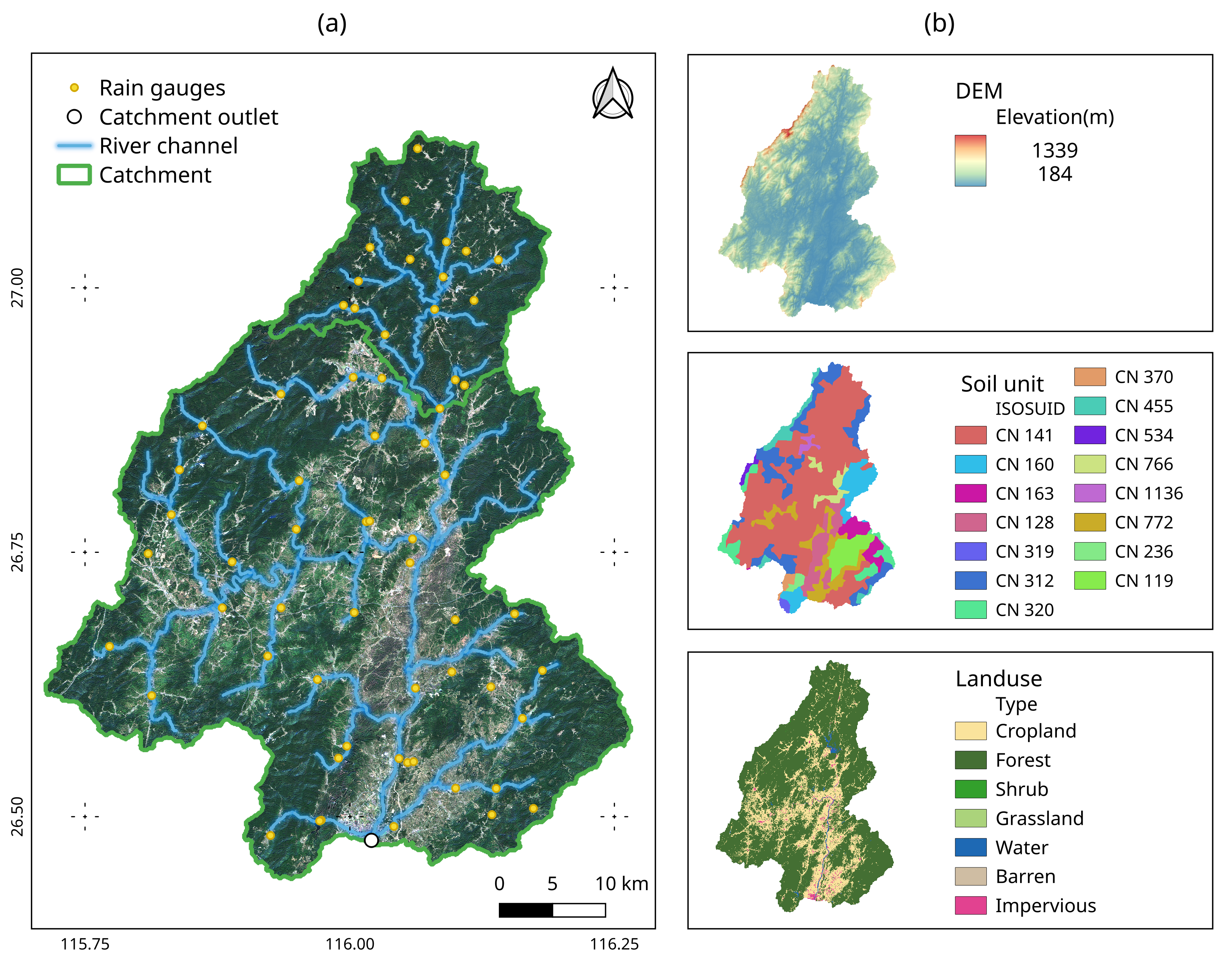
Figure 2 is the overview of the Ningdu catchment, showing its river network, rain gauge distribution, DEM, soil type, and land use. The catchment lies between 35 and 693 m in elevation and consists of river networks, which are tributaries of the Mei River. The catchment is located in the subtropical monsoon region, with forest and cropland as the primary land-use types. Human influence on the hydrological processes is relatively limited. According to the SOTER China database [
8], there are 15 soil units in the catchment, with Haplic Acrisols being the predominant soil type. The Ningdu catchment is well-managed, it has a 62 rain gauge network, and long-time series hourly rainfall observations for the past few years have been collected.
2.2. Flood Events Data and Model Construction Data
Sixteen typical flood event data (time series of precipitation in each rain gauge and flow observation in catchment outlet) are extracted from the long time series of rain gauge observation from 2013 to 2017.
Table 1 describes the flood events’ characteristics. The flood event dataset encompasses floods of varying magnitudes, ranging from large to small, and the flood durations span from 119 h to 527 h.
Event 2016-11-19 is chosen for parameter optimization, as it is a medium twin peak flood with a smooth flood hydrograph, which is relatively information-rich and less noisy for model parameter optimization. The other 15 events are used for model performance testing.
The basic structure of the Liuxihe model is constructed by DEM, soil, and land-use remote-sensing products. In this study, the 90 m SRTMv4 dataset [
23] is used for the catchment DEM, model parameter slope and flow direction can be calculated from the DEM. For land-use data, a 30 m land-use product by Yang and Huang [
6] is warped (resampled and aligned) to the resolution of DEM, and the model slope cell parameter evaporation coefficient and roughness coefficient are estimated according to the land-use of the cell. For soil data, the SOTER China database [
8] is used. Soil-related parameters of the model could be calculated by a soil water characteristic calculator developed by Saxton and Rawls [
24], according to the profile component of the soil. The initial values of landuse-related and soil-related parameters for the study catchment are provided in the
Appendix A.
2.3. Liuxihe Model and Its Parameter Optimization Method
Liuxihe model is a productive PBDHM for mesoscale catchment flood forecasting, which has been applied to flood forecasting in many catchments in Southern China [
25,
26,
27,
28,
29]. The following is a brief anatomy of the Liuxihe model and further details about the model can be found in [
13].
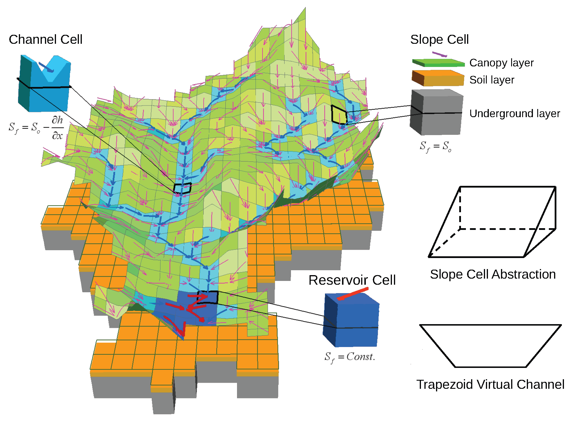
As a PBDHM, the Liuxihe model’s distributed structure is derived from DEM; the grid unit of the DEM is the minimum calculation unit of the model, which is also called cells in the GIS context. Each cell has its attributes, i.e., the model parameters. The Liuxihe model has a few parameters for its simplicity, which fall into four categories, DEM-derived parameters (cell class, slope, flow direction), soil parameters (thickness, saturation hydraulic conductivity, saturated soil water content, field water capacity, wilting point, porosity coefficient, infiltration intensity), land-use parameters (evaporation coefficient, roughness coefficient), and channel parameters (bottom width, bottom slope, side slope, channel roughness). By dividing the catchment into slope cell, channel cell, and reservoir cell horizontally and canopy layer, soil layer, and underground layer vertically, the Liuxihe model couples three subroutines on evaporation, flow generation, and flow convergence to describe the flood process response to a rain event.
Figure 3 illustrates the structure of the Liuxihe model.
Though the parameters of PBDHMs derived from remote-sensing data are near to real value, revising the parameters is still needed in model building [
30,
31], due to the uncertainty in geography data. Many PBDHMs are equipped with parameter optimization/calibration methods [
31,
32,
33], which need observed flow data to tune model parameters responding to rainfall input as close to reality as possible. As with many PBDHMs, the Liuxihe model is equipped with its parameter optimization method [
31], which is based on the particle swarm optimization (PSO) algorithm [
34]. The Liuxihe Model adopts a scaling law to optimize its parameters. As mentioned earlier, the model’s initial parameters are derived from remote-sensing data, which carry inherent uncertainties. To account for potential deviations, the parameters can be scaled within a range of 0.5 to 1.5 times their initial values and constrained by physical significance. Different particles in the swarm represent the scaling coefficients of the model parameters and move within the solution space. These particles evaluate the quality of their positions using an objective function (also called fit in the PSO context, Equation (
1) is used in this study) and adjust their direction and speed accordingly, ultimately converging towards an optimal state. The final optimized model parameters are obtained by multiplying the initial parameters by the scaling coefficients, ensuring that the parameters remain physically meaningful.
2.4. Rainfall Spatial Interpolation Methods
There are many spatial interpolation methods to generate a distributed rainfall input from gauge observation point data, but most of them are focused on a day scale or month scale [
35,
36], or are too complicated for application on an hourly scale. Take Ordinary Kriging, for example, data with weak spatial heterogeneity may face difficulty fitting the semivariogram automatically, resulting in unreliable spatial predictions [
37]; this phenomenon often occurs when there are few gauges and minor rainfall, leading to inconsistency in the interpolated rainfall surfaces. In flood forecasting, operators often lack sufficient knowledge to handle these conditions. For these reasons, simple and automatic methods are still commonly used in practice. Considering the ease of use and applicability, this study selects THI, IDW, and GWR for research. They are both representative and widely used in practice. The theoretical backgrounds are briefly introduced below. More detailed information can be found in [
38,
39,
40].
The theory of THI is simple, as in Equation (
2), rainfall that occurs in one cell
c is generalized the same as its nearest gauges
g’s measurement
.
IDW assumes that gauges closer to the location of interest have more influence on the estimated value. The method calculates a weighted average of gauge observations, with weights inversely proportional to their distance from the target location, as shown in Equation (
3).
where
D is a function that describes distances between Cell
c and gauge
g; the Euclidean distance is commonly used.
GWR accounts for the spatial heterogeneity inherent in rainfall patterns. Unlike traditional regression, GWR accounts for geographic location, allowing coefficients to vary across space. It fits a regression model at each location using nearby observations, weighted by their distance, thus capturing local variations and providing more accurate spatial predictions. For consistency with THI and IDW, who only consider distance in rainfall interpolation, the form of GWR without considering other variables is used in this study. Rainfall in one cell
c can be predicted as in Equation (
4).
where
is the solved regression coefficients,
is bandwidth calculated by the AIC method [
40], and
is the spatial weight which could be calculated by Equation (
5).
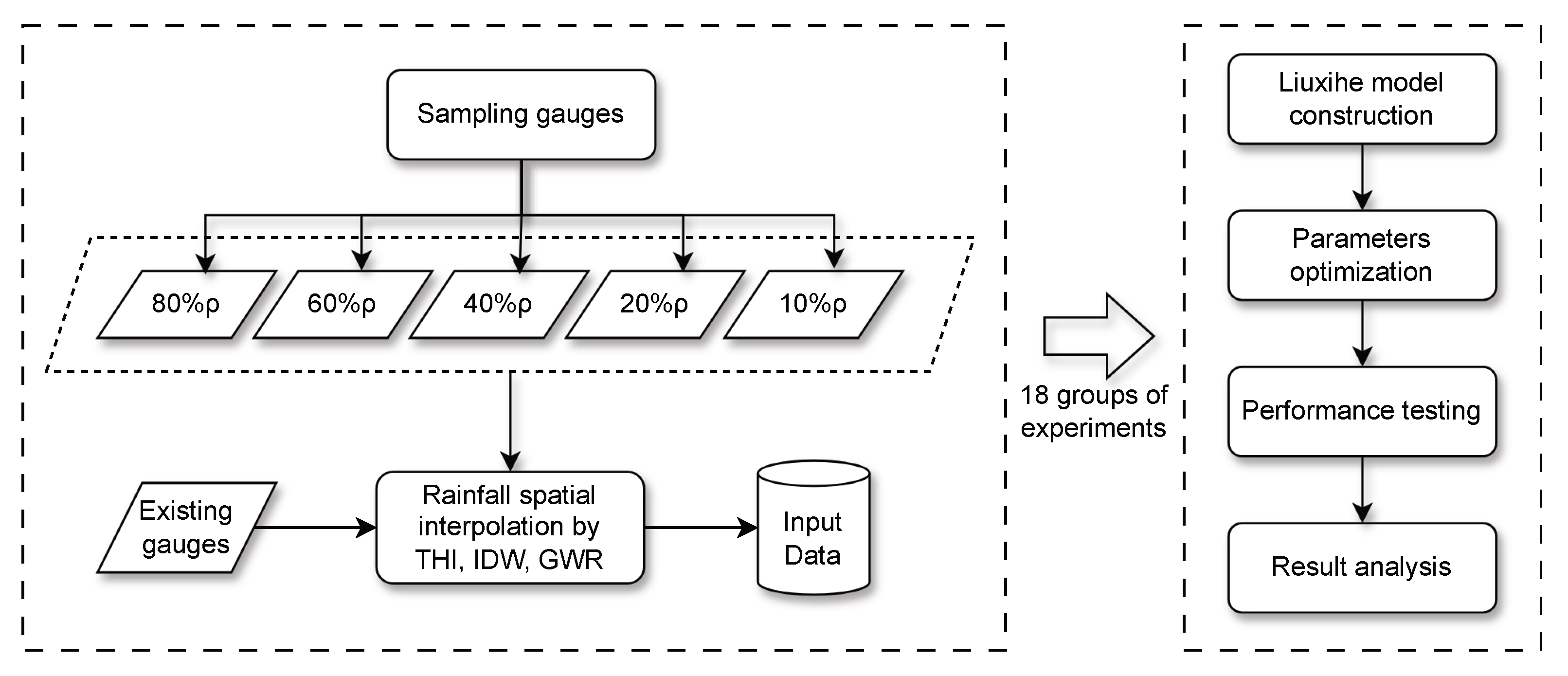
2.5. Experimental Settings
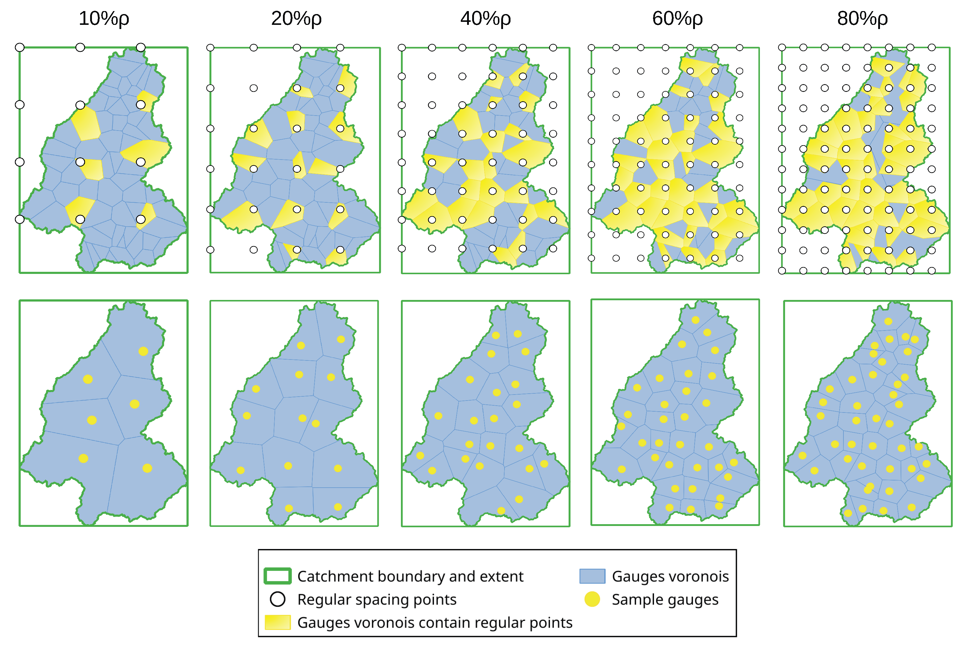
As mentioned earlier in the introduction, five rain gauge density conditions are derived from existing gauge distribution by an algorithm based on the distance of gauges. Algorithm 1 illustrated these procedures and
Figure 4 further depicted the process visually.
| Algorithm 1 Sampling Scheme |
|
When installing rain gauges within a catchment, it is common to maximize their effectiveness by distributing rain gauges as evenly as possible when conditions permit. Without considering special circumstances, the density of rain gauges in a catchment can be estimated by dividing the catchment area by the number of gauges. Some GIS tricks can be employed to generate different rain gauge density scenarios. In Algorithm 1, it is assumed that rain gauge density can be measured by the average distance between gauges. By scaling the estimated average distance of existing gauges with factors of 0.8, 0.6, 0.4, 0.2, and 0.1, regular spacing points that mimic the distribution of sampled gauges in these scenarios can be generated. If an existing rain gauge whose Voronoi polygon contains a regular spacing point, this gauge will be chosen to use. This approach simplifies real-world scenarios based on the Voronoi polygon theory. Ultimately, five generated rain gauge density scenarios and 1 existing gauge scenario are present, corresponding to the number of gauges being used are 62, 41, 32, 22, 13, and 6, and the estimated control area of each gauge is 38 km2, 57 km2, 74 km2, 107 km2, 182 km2, and 394 km2, respectively. Notice that from 100% density to 80% density, up to 20 gauges are excluded from the sample. This occurs because existing rain gauges are not perfectly uniformly distributed, some closely spaced gauges are filtered out by the algorithm.
Gauges are selected from a scale of the average distance, which could be regarded as a scale of gauge density. For simplicity, use an abbreviated notation for experiment naming, e.g., “100P” represents the experiment on existing gauge density (), “THI80P” represents the experiment on gauges sampled by intersection with spacing points () and use THI to interpolate distributed rainfall surfaces. Combining six gauge density conditions with three spatial interpolation methods, there are 18 scenarios in total. The model parameters are optimized only for scenarios THI100P, IDW100P and GWR100P in the same PSO settings, as the characteristics of their interpolated surface are different. The performance of the experiments THI100P, IDW100P, and GWR100P will be evaluated first, serving as the reference baseline for observing how the model’s performance changes under varying rain gauge density conditions.
The evaluators chosen to compare the model performance are Kling–Gupta Efficiency (KGE) [
41], Nash–Sutcliffe Efficiency (NSE), peak relative error (PRE), and absolute peak time error (APTE). KGE and NSE evaluate the overall agreement between the predicted and observed hydrographs. While NSE focuses on how well the predictions capture the observed variability, KGE offers a more balanced evaluation by incorporating correlation, bias, and variability into the assessment and is less affected by extreme values [
42]. PRE and APTE assess the model’s flood forecasting performance from the perspective of peak flow, while the former focuses on the magnitude of the peak flow, and the latter on the timing of the peak. These four evaluators together provide a comprehensive comparison of the model’s performance. Their definitions are as follows.
where
r is the Pearson correlation coefficient,
is the ratio of the mean of simulated flows and observed flows defined as
, and
is the ratio of the standard deviation of simulated flow and observed flows defined as
.
where
is the observed flow at time
t,
is the simulated flow at time
t,
is the mean of observed flows over the simulation period,
n is the number of observations.
where
is the observed flow peak, and
is the simulated flow peak.
where
and
are flood peak occurrence time of the observed flow and simulated flow, respectively.


