Predicting the Dynamic of Debris Flow Based on Viscoplastic Theory and Support Vector Regression

Abstract

The prediction of debris flows is essential for safeguarding infrastructure and minimizing the economic losses associated with the hazards. Traditional empirical and theoretical models, while providing foundational insights, often struggle to capture the complex and nonlinear behaviors inherent in debris flows. This study aims to enhance debris flow prediction by integrating theoretical modeling with data-driven approaches. We model debris flow as a viscoplastic fluid, employing the Herschel–Bulkley rheological model to describe its behavior. By combining the kinematic wave model with lubrication theory, we develop a comprehensive theoretical framework that encapsulates the mechanical physics of debris flows and identifies key governing parameters. Numerical solutions of this theoretical model are utilized to generate an extensive training dataset, which is subsequently used to train a support vector regression (SVR) model. The SVR model targets slide depth and velocity upon impact, using explanatory variables including yield stress, material density, source area depth and length, and slope length. The model demonstrates high predictive accuracy, achieving coefficients of determination $R^2$ of 0.956 for slide depth and 0.911 for slide velocity at impact. Additionally, the relative residuals $\sigma$ are primarily distributed within the range of −0.05 to 0.05 for both slide depth and slide velocity upon impact. These results indicate that the proposed hybrid model not only incorporates the fundamental physical mechanisms governing debris flows but also significantly enhances predictive performance through data-driven optimization. This study underscores the critical advantage of merging physical models with machine learning techniques, offering a robust tool for improved debris flow prediction and risk assessment, which can inform the development of more effective early warning systems and mitigation measures.

1. Introduction

Mountain torrents, characterized by their rapid water flow and steep gradients, are a major trigger for debris flows in mountainous regions. These debris flows, characterized by their rapid movement and high destructive potential, pose significant risks to both infrastructure and human lives [1,2,3]. The intense water flow of mountain torrents mobilizes loose sediments and organic material, transforming into destructive debris flows. Debris flows can vary in speed depending on factors such as water content, slope angle, and the amount of material involved [4,5]. The unpredictable nature of the widespread destruction of debris flows necessitates understanding the physical mechanisms driving debris flows and developing prediction models to inform early warning systems and mitigation strategies.

Research on debris flow analysis and prediction has a long history, evolving from empirical methods and simplified numerical models to more sophisticated theoretical frameworks. Early studies investigated the rheological properties of debris flows, highlighting the effects of sediment concentration and water content on viscosity [6]. These seminal works laid the groundwork for subsequent model developments [7]. Recent advancements in hazard chain prediction have integrated rainfall-induced shallow landslides with subsequent debris flows to provide a more comprehensive assessment of geohazard risks [8]. Later research underscored the importance of accounting for both viscous and plastic behaviors in debris flow dynamics, such as providing in-depth analyses of the rheological properties of debris flows and debris flows, discussing their complex flow behavior [9]. Takahashi further explored the mechanical aspects of debris flows and developed models to predict their behavior under different conditions [9]. Recent advancements in debris flow modeling have markedly improved prediction accuracy and deepened the understanding of flow dynamics. For instance, the adoption of advanced rheological models has shed light on the impact of specific parameters, offering a more detailed perspective on the intricate behaviors of debris flows [10,11].

Debris flows are influenced by a multitude of factors, including rainfall, soil properties, vegetation cover, and human activities [12]. Capturing the nonlinear interactions among these factors in a single theoretical model is challenging. Most theoretical models rely on simplifications and assumptions that may not accurately capture the real-world complexity of debris flows [13,14]. Given the limitations of theoretical and numerical models, there is a growing need to develop data-driven prediction methods that leverage real-time monitoring data. These models can continuously learn and adapt from new data, improving their predictive accuracy over time. They can also capture complex, nonlinear interactions between various factors influencing debris flows, which are often difficult to model explicitly using traditional approaches [15].

As data-driven methods, machine learning techniques are increasingly used to model real-time monitoring data or remote sensing data, to predict the risk and potential affects of debris flows [16,17,18]. These techniques leverage the vast amounts of data collected from various sources to develop predictive models that can provide timely warnings and risk assessments. Korup and Stolle (2014) reviewed the application of machine learning techniques in the prediction of landslides, highlighting their potential to improve accuracy and efficiency in hazard assessment [19]. Techniques such as support vector machines (SVM), artificial neural networks (ANN), and random forests (RF) have been employed to classify and predict landslide occurrences based on historical data and environmental variables [20,21,22]. In addition, recent advancements in remote sensing technologies, such as LiDAR and satellite imagery, have enhanced the ability to gather high-resolution data over large and inaccessible areas [23,24,25]. These technologies provide critical inputs for machine learning models, enabling the detection of subtle changes in topography and land cover that may precede debris flows [26]. However, the effectiveness of data-driven models is often contingent upon the availability and quality of data [27]. These models typically require extensive datasets to train and validate the algorithms, which may not always be available in regions prone to debris flows due to the high financial cost of monitoring sensors. The reliance on comprehensive monitoring data limits the applicability of data-driven methods in less-instrumented areas and necessitates robust data collection infrastructure. Furthermore, challenges such as data heterogeneity, missing values, and the need for continuous updates to the models as new data becomes available can impact the reliability of predictions.

The objective of this study is to develop an advanced debris flow prediction model by combining theoretical analysis with the data-driven method. For the theoretical part, we seek to capture the essential physical mechanisms driving debris flow dynamics and determine the dominating factors governing the physical process. We consider the debris flow as a viscoplastic fluid whose rheological behavior follows the Herschel–Bulkley model. The integration of lubrication theory and the kinematic wave model within this framework enables a detailed representation of the rheology of viscoplastic fluid. Lubrication theory is adept at modeling thin and viscous fluid layers, accounting for the effects of viscosity and pressure gradients, whereas the kinematic wave model is effective in describing the movement of shallow waves influenced by gravity and surface slopes [28,29]. The numerical solutions of the dominant factors that derived from the theoretical foundations are subsequently used to train the support vector regression (SVR) model, providing a robust data-driven tool for predicting debris flow events. Through this interdisciplinary approach, we aim to advance the current state of debris flow prediction, incorporating the underlying dynamics.

The present article is organized as follows. Section 3 introduces the theoretical aspects of viscoplasticity as applied to debris flows and describes the math implementation of the SVR model. Section 4 presents the numerical solution of the theoretical model combining the lubrication model and kinematic wave model, and exhibits the prediction results of the SVR model developed based on the dataset of numerical results. Section 5 discusses the implications of the results and highlights the limitations of the current study. Finally, Section 6 summarizes the key findings and suggests directions for future research.

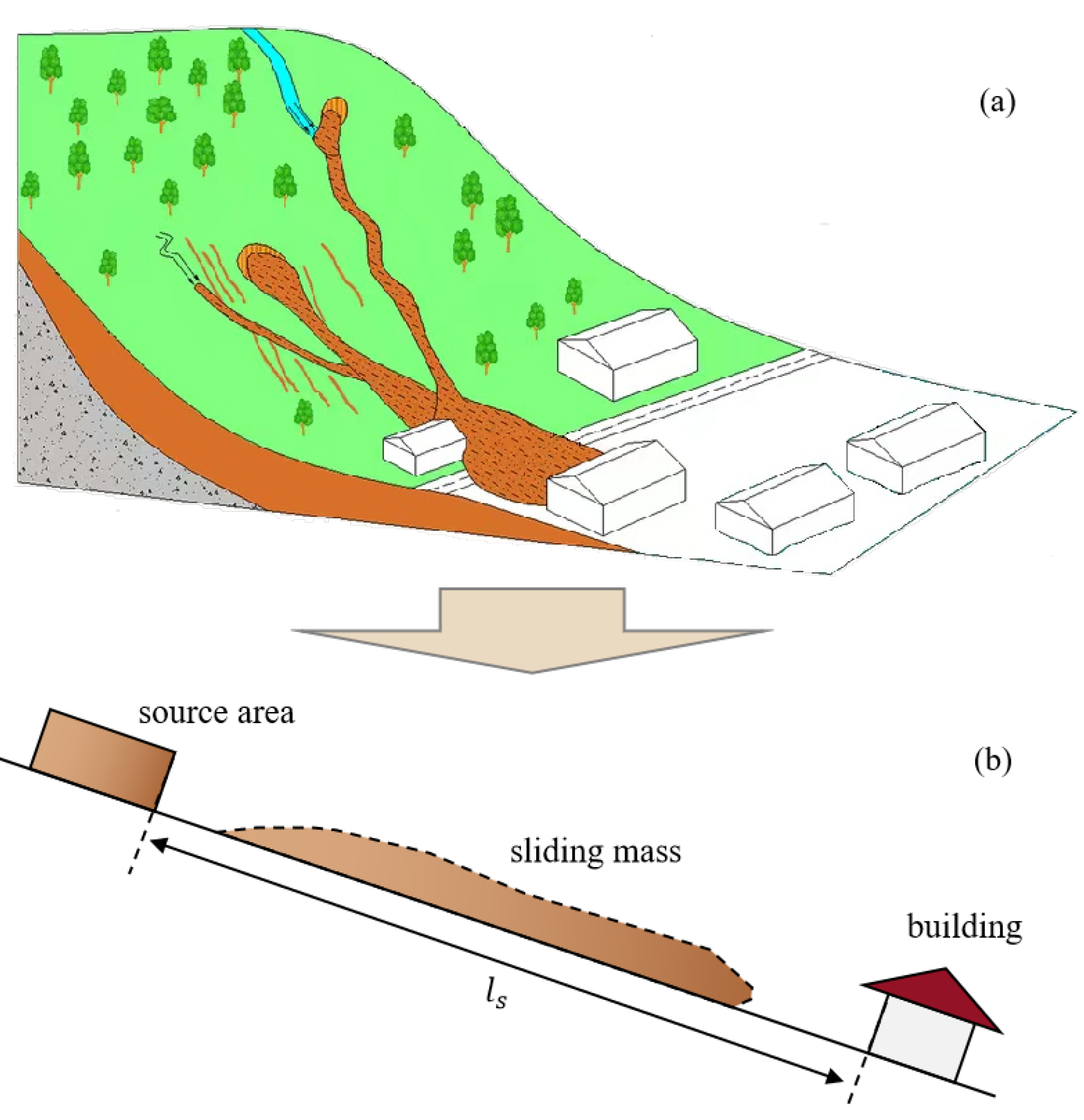
2. Simplification of the Issue

2.1. Physical Model

We give insights on the dynamics of debris flows and the potential impact on buildings downslope from the source areas. The issue can be simplified as examining the thickness and depth-averaged velocity of the debris flow as it reaches a building located at a distance $l_s$ from the initial source areas. The simplified physical model is illustrated in Figure 1. The simplified physical model serves as a framework for understanding the critical parameters that govern the impact of debris flows on buildings. By focusing on the thickness and depth-averaged velocity of the sliding mass, this study aims to provide insights for predicting hazards and implementing effective mitigation strategies.

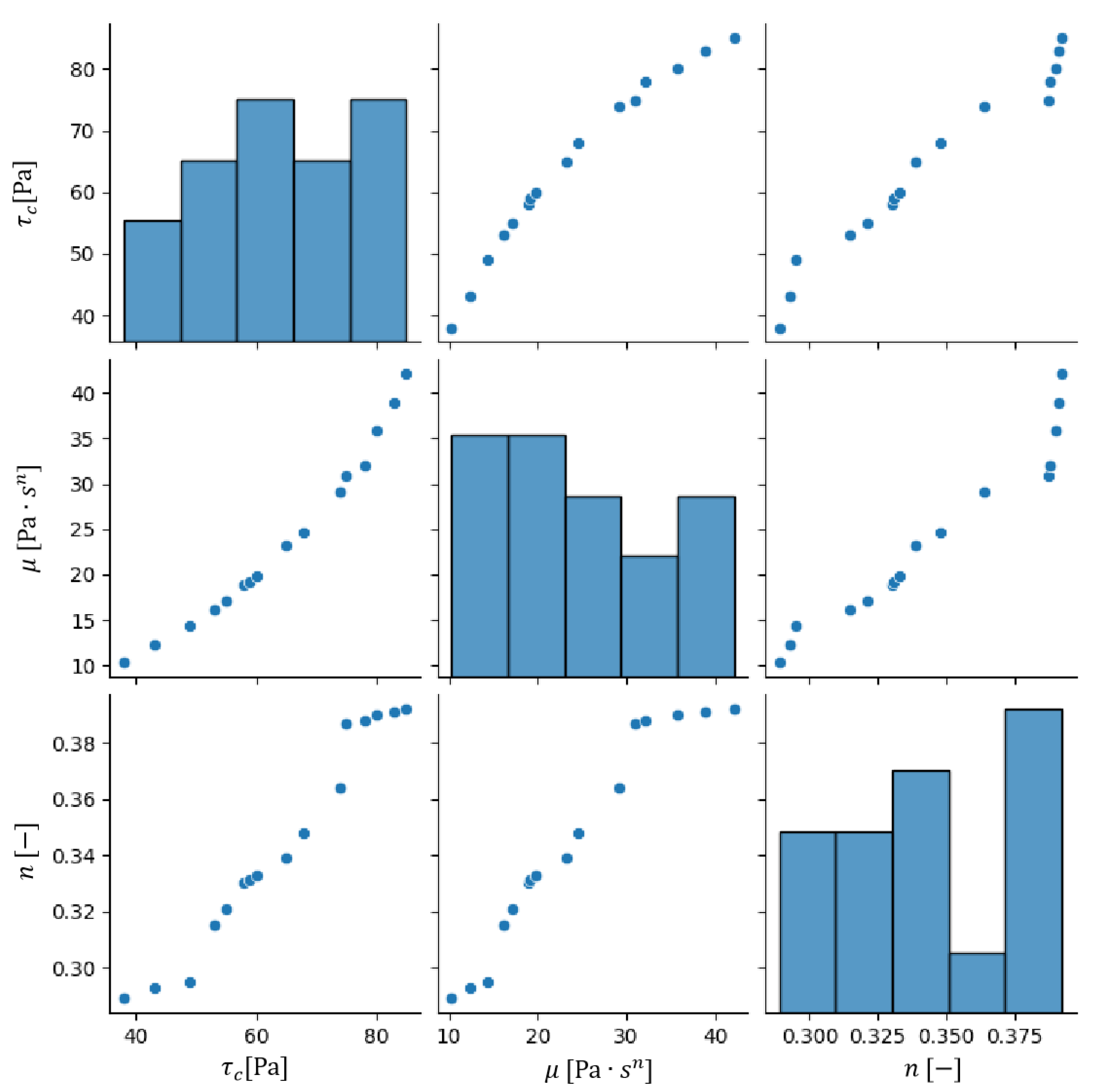
2.2. Material Modeling

The characteristics of flows with increasing solid content have been investigated experimentally. Flows with low solid fractions are primarily influenced by viscous stresses, resulting in greater mobility upon impact. In contrast, flows with higher solid fractions are dominated by internal friction. In this case, the debris flow is modeled as a homogeneous viscoplastic fluid within the Herschel–Bulkley framework, effectively integrating the combined effects of varied sediment sizes, vegetation, foreign materials, and water content into the yield stress and plastic viscosity parameters. This homogenization allows for the simulation of mudflow-like debris flows on gentle slopes by capturing the essential rheological behaviors observed in such flows [30,31]. The Herschel–Bulkley model is commonly employed to describe the rheological behavior of debris flow, whose expression for simple-shear flows can be written as follows:

$$\tau ={\tau }_c+\mu {\dot{\gamma }}^n$$

(1)

where ${\tau }_c$ is the yield stress, the stress threshold below which the material behaves like a solid and above which it flows like a fluid; $\dot{\gamma }$ is the shear rate, $\mu$ is the consistency, and n is a power-law index that reflects shear thinning or shear thickening. In this study, we assume that the rheological behavior of debris flow follows the Herschel–Bulkley model. Note that assuming debris flow as a viscoplastic fluid remains controversial in the scientific field; however, we do not address this controversy here. We conducted the rheological measurements using a Bohlin Gemini rheometer equipped with striated parallel plates (diameter: 25 mm, gap size: 1 mm). The rheological parameters were fitted using the Herschel–Bulkley equation with these measurements.

Table 1. Rheological parameters ${\tau }_c$, $\mu$, and n adopted in this study.

${\mathit{\tau }}_{\mathit{c}}$ [Pa]	$\mathit{\mu }$ [Pa · sn]	n [-]
38	10.3	0.289
49	14.4	0.295
55	17.1	0.321
68	24.6	0.348
75	30.9	0.387
80	35.8	0.390
85	42.1	0.392

shows the rheological parameters ${\tau }_c$, $\mu$, and n adopted in this study.

3. Prediction Model Development

In this study, we combine the kinematic wave model with lubrication theory to develop a comprehensive theoretical framework that captures the mechanical physics of debris flows. This theoretical model helps identify the key governing parameters that influence debris flow behavior. Numerical solutions derived from this model are used to generate an extensive training dataset, which serves as the foundation for the data-driven component of the research. The dataset is then used to train a support vector regression (SVR) model, which predicts critical outcomes such as slide depth and velocity upon impact. The SVR model uses explanatory variables including yield stress, material density, source area depth and length, and slope length to make these predictions. This approach effectively integrates the physical model with the data-driven SVR model, where the former provides the theoretical foundation and key parameters, while the latter refines predictions based on empirical data.

3.1. Theoretical Analysis Based on Lubrication Model and Kinematic Wave Model

Figure 2 shows the sketch of the sliding mass at rest and moving along the slope. We used a coordinate system $(\widehat{x},\widehat{y})$, where $\widehat{x}$ denotes the downstream coordinate measured from the top of the plane and $\widehat{y}$ denotes the coordinate normal to the slope. The interest is to determine $s(\widehat{x}=l_s,\widehat{t})$ and $u(\widehat{x}=l_s,\widehat{t})$, where $l_s$ is the distance from the origin to the objective position, and $\widehat{t}$ is time.

The initial flow depth is given by

$$s(\widehat{x})=s_g+(\widehat{x}-l_0)tan\theta$$

(2)

and the initial flow depth at the lock gate $s_g$ is given by

$$s_g=V_I/l_0+{\displaystyle \frac{1}{2}}{l}_{0}tan\theta$$

(3)

where $V_I$ is the volume of the slide material in the reservoir and $l_0$ denotes the length of the slide material in the reservoir.

We first considered a steady uniform flow of viscoplastic fluid over an inclined surface. The rheological behavior of the viscoplastic fluid is described by the Herschel–Bulkley equation (see Equation (1)) [2]. Independently of the constitutive equation, the shear stress distribution throughout the depth is

$$\tau (\widehat{y})={\rho }_{s}g(s-\widehat{y})sin\theta$$

(4)

where s denotes the flow depth, ${\rho }_s$ is the density of the slide material, and g is the gravitational acceleration. The no-slip condition was assumed for the stream-wise velocity component u at the bottom, that is, $u(\widehat{y}=0)=0$. The integration of the constitutive Equation (1) provides the cross-stream velocity profile:

$$u(\widehat{y})={\displaystyle \frac{nA}{n+1}}\left\{\begin{array}{ccc}\left(Y_0^{1+1/n}-{(Y_0-\widehat{y})}^{1-1/n}\right)\hfill & & \widehat{y}\le Y_0\hfill \\ Y_0^{1+1/n}\hfill & & \widehat{y}\ge Y_0\hfill \end{array}\right.$$

(5)

with

$$Y_0=s-s_c,A={\left({\displaystyle \frac{{\rho }_{s}gsin\theta }{\mu }}\right)}^{1/n},s_c={\tau }_c/\left({\rho }_{s}gsin\theta \right)$$

(6)

where $s_c$ denotes the critical flow depth, that is, no steady uniform flow is possible for $s<s_c$ and $Y_0$ denotes the position of the yield surface with $\widehat{y}<Y_0$ the sheared region and $\widehat{y}>Y_0$ the unyielding region. A further integration leads to the depth-averaged velocity:

$$\overline{u}={\displaystyle \frac{nA}{(n+1)(2n+1)}}{\displaystyle \frac{s(n+1)+n{s}_c}{s}}{Y}_0^{1+1/n}$$

(7)

When the flow is slightly non-uniform, the shear stress alters as a result of the changes in the free-surface gradient. A common approach is to start from the Cauchy momentum balance equation, in which the inertia terms have been neglected together with the normal stress gradient [32]. With the assumption of negligible inertia, the downstream projection of the momentum balance equation reads

$$0={\rho }_{s}gsin\theta -{\displaystyle \frac{\partial p}{\partial \widehat{x}}}+{\displaystyle \frac{\partial \tau }{\widehat{y}}}$$

(8)

and the pressure is found to be hydrostatic to the leading order $p={\rho }_{s}g(s-\widehat{y})cos\theta$. Then, the shear stress distribution reads

$$\tau ={\rho }_{s}g(s-\widehat{y})cos\theta \left(tan\theta -{\displaystyle \frac{\partial s}{\partial \widehat{x}}}\right)$$

(9)

Substituting Equation (9) into Equation (1) and integrating it yields

$$u(\widehat{y})={\displaystyle \frac{nK}{n+1}}{\left(tan\theta -{\displaystyle \frac{s}{\widehat{x}}}\right)}^{1/n}\left\{\begin{array}{ccc}\left(Y_0^{1+1/n}-{\left(Y_0-\widehat{y}\right)}^{1+1/n}\right)\hfill & & \widehat{y}\le Y_0\hfill \\ Y_0^{1+1/n}\hfill & & \widehat{y}\ge Y_0\hfill \end{array}\right.$$

(10)

with the parameter K and the updated yield surface position $Y_0$ as follows:

$$K=\rho gsin\theta /k,Y_0=\max (0,s-{\tau }_c/(\rho gcos\theta (tan\theta -{\partial }_{x}s)))$$

(11)

The critical depth is $s_c={\tau }_c/\left({\rho }_{s}gsin\theta \right)$. A further integration leads to the depth-averaged velocity for non-uniform flow:

$$\overline{u}={\displaystyle \frac{nK}{(n+1)(2n+1)}}{\left(tan\theta -{\displaystyle \frac{\partial s}{\partial \widehat{x}}}\right)}^{1/n}{\displaystyle \frac{s(n+1)+n{s}_c}{s}}{Y}_0^{1+1/n}$$

(12)

Using Equation (12) requires an equation specifying the gradient of the free surface ${\partial }_{x}s(\widehat{x},\widehat{t})$. We then used the kinematic wave model to evaluate $s(\widehat{x},\widehat{t})$. The kinematic wave approximation assumes that the fluid is locally uniform, that is, $\overline{u}$ is given by Equation (7). The bulk mass balance ${\displaystyle \frac{\partial s}{\partial \widehat{t}}}+{\displaystyle \frac{\partial s\overline{u}}{\widehat{x}}}=0$ provides the governing equation for s:

$${\displaystyle \frac{\partial s}{\partial \widehat{t}}}+f^{\prime }(s){\displaystyle \frac{\partial s}{\partial \widehat{x}}}=0$$

(13)

$$\mathrm{with}{f}^{\prime }(s)=As{(s-s_c)}^{1/n},\mathrm{and}A={\left({\displaystyle \frac{\rho gsin\theta }{\mu }}\right)}^{1/n}$$

(14)

This hyperbolic nonlinear advection equation can be solved easily using the method of characteristics. Equation (13) can be put into a characteristic form ${\displaystyle \frac{ds}{d\widehat{t}}}=0$ along the characteristic curve ${\displaystyle \frac{d\widehat{x}}{d\widehat{t}}}=f^{\prime }(s)$. These initial characteristic curves are straight lines whose slope is dictated by the initial depth:

$$\widehat{x}=f^{\prime }(s({\widehat{x}}_0))\widehat{t}+{\widehat{x}}_0$$

(15)

where $s_0({\widehat{x}}_0)$, the initial value of s at ${\widehat{x}}_0$, is given by Equations (2) and (3). As $h=h_0$ along the characteristic curve, using Equation (2) to eliminate ${\widehat{x}}_0$, an implicit equation for s can be obtained:

$$\widehat{x}=As{(s-s_c)}^{1/n}\widehat{t}+(s-s_g)cot\theta +l_0$$

(16)

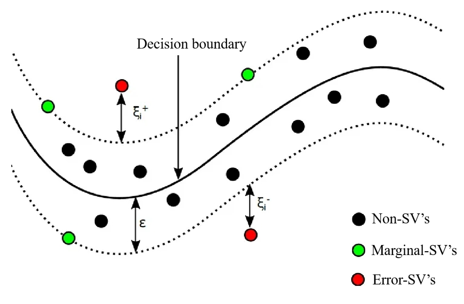
3.2. Mathematical Procedure of Data Modeling Using Support Vector Regression

After generating a dataset using key parameters extracted from numerical solutions of the theoretical model presented in Section 3.1, we then model the dataset using support vector regression (SVR) model, which is a supervised learning algorithm used for regression tasks aiming to find a function that deviates from the actual observed values by a value no greater than a specified margin [33,34]. It leverages the principles of the support vector machines model for classification and adapted for regression problems. Figure 3 illustrates the flowchart of the SVR model.

Here is the mathematical foundation of SVR [35]. Given a training dataset ${\left\{(x_i,y_i)\right\}}_{i=1}^N$, where $x_i\in {\mathbb{R}}^d$ represents the feature vectors and $y_i\in \mathbb{R}$ represents the target values, the objective of SVR is to find a function $f(x)$ that approximates the target values $y_i$ with a tolerance margin $ϵ$.

The function $f(x)$ in SVR is typically expressed as

$$f(x)=w·\varphi (x)+b$$

(17)

where w is the weight vector, $\varphi (x)$ is a nonlinear mapping function that transforms the input data into a higher-dimensional space, and b is the bias term.

SVR aims reducing the error by determining the hyperplane and minimising the range between the predicted and the observed values using an $ϵ$-insensitive loss function, which ignores errors within a specified margin $ϵ$, as shown in Figure 4. The loss function for SVR is defined as

$$L_{ϵ}(y,f(x))=max\{0,|y-f(x)|-ϵ\}$$

(18)

The optimization problem in SVR is formulated to minimize the following objective:

$${\displaystyle \frac{1}{2}}{\parallel w\parallel }^2+C{\displaystyle \sum _{i=1}^N}{L}_{ϵ}(y_i,f(x_i))$$

(19)

where ${\parallel w\parallel }^2$ is the regularization term that aims to keep the model weights small, and C is a regularization parameter that determines the trade-off between the flatness of the function and the tolerance for deviations larger than $ϵ$.

To handle deviations larger than $ϵ$, slack variables ${\xi }_i$ and ${\xi }_i^{*}$ are introduced, representing the degree of deviation from the margin:

$$\begin{array}{cc}\hfill y_i-(w·\varphi (x_i)+b)& \le ϵ+{\xi }_i\hfill \\ \hfill (w·\varphi (x_i)+b)-y_i& \le ϵ+{\xi }_i^{*}\hfill \\ \hfill {\xi }_i,{\xi }_i^{*}& \ge 0\hfill \end{array}$$

(20)

Thus, the optimization problem becomes

$$\underset{w,b,\xi ,{\xi }^{*}}{min}{\displaystyle \frac{1}{2}}{\parallel w\parallel }^2+C{\displaystyle \sum _{i=1}^N}({\xi }_i+{\xi }_i^{*})$$

(21)

subject to

$$\begin{array}{cc}\hfill y_i-(w·\varphi (x_i)+b)& \le ϵ+{\xi }_i\hfill \\ \hfill (w·\varphi (x_i)+b)-y_i& \le ϵ+{\xi }_i^{*}\hfill \\ \hfill {\xi }_i,{\xi }_i^{*}& \ge 0\hfill \end{array}$$

(22)

To solve the primal optimization problem, it is more practical to convert it into its dual form using Lagrange multipliers. The dual problem is

$$\begin{array}{c}\hfill \underset{\alpha ,{\alpha }^{*}}{max}\{-{\displaystyle \frac{1}{2}}{\displaystyle \sum _{i,j=1}^N}({\alpha }_i-{\alpha }_i^{*})({\alpha }_j-{\alpha }_j^{*})K(x_i,x_j)\\ \hfill +{\displaystyle \sum _{i=1}^N}{y}_i({\alpha }_i-{\alpha }_i^{*})-ϵ{\displaystyle \sum _{i=1}^N}({\alpha }_i+{\alpha }_i^{*})\}\end{array}$$

(23)

subject to

$${\displaystyle \sum _{i=1}^N}({\alpha }_i-{\alpha }_i^{*})=0$$

(24)

$$0\le {\alpha }_i,{\alpha }_i^{*}\le C$$

(25)

Here, ${\alpha }_i$ and ${\alpha }_i^{*}$ are the Lagrange multipliers, and $K(x_i,x_j)=\varphi (x_i)·\varphi (x_j)$ is the kernel function that enables the transformation of input data into a higher-dimensional space without explicit computation.

Common kernel functions include

$$K(x_i,x_j)=x_i·x_j(\mathrm{linear})$$

(26)

$$K(x_i,x_j)={(x_i·x_j+1)}^p(\mathrm{polynomial})$$

(27)

$$K(x_i,x_j)=exp(-\gamma \parallel x_i-x_j{\parallel }^2)(\mathrm{radial}\mathrm{basis}\mathrm{function})$$

(28)

The solution to the dual problem provides the optimal Lagrange multipliers ${\alpha }_i$ and ${\alpha }_i^{*}$, which are used to express the weight vector w as

$$w={\displaystyle \sum _{i=1}^N}({\alpha }_i-{\alpha }_i^{*})\varphi (x_i)$$

(29)

The final prediction function is

$$f(x)={\displaystyle \sum _{i=1}^N}({\alpha }_i-{\alpha }_i^{*})K(x_i,x)+b$$

(30)

The bias term b is determined using the Karush–Kuhn–Tucker conditions, which ensure the solution satisfies the constraints of the optimization problem.

Table 2. Simulation parameters for SVR.

Parameters	Value
Regularization parameter C	0.01
tolerance $ϵ$	0.01
Kernel function	Polynomial function

shows the initial settings of parameters in SVR.

4. Results

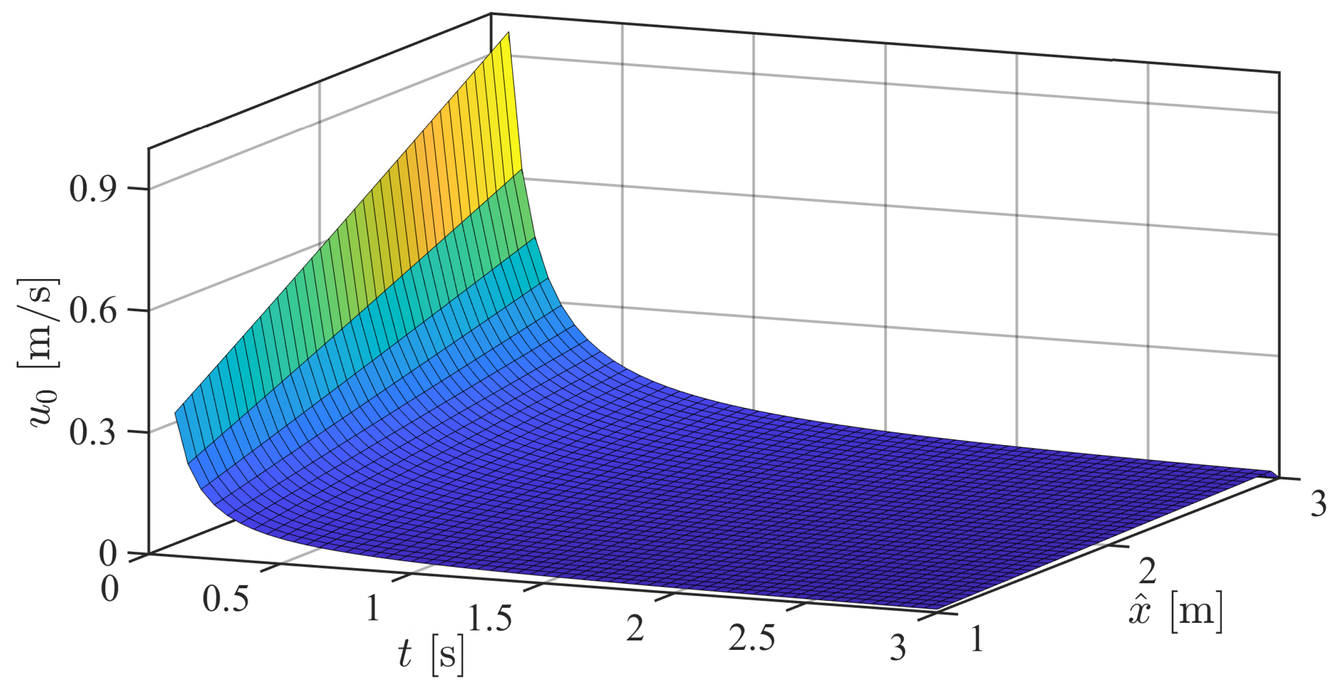
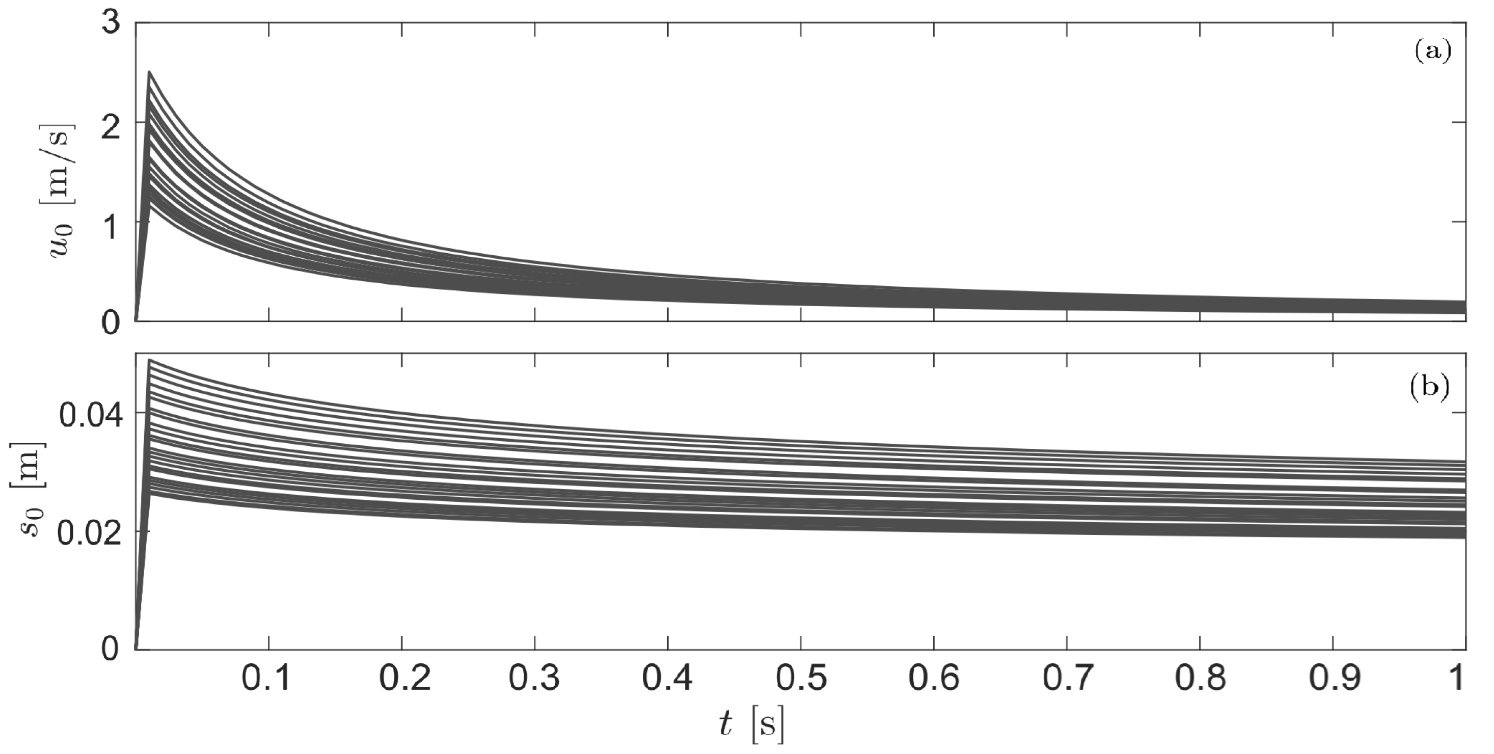
4.1. Numerical Solution of the Theoretical Model

Section 3.1 presented theoretical expressions for the time series data of the slide’s thickness $s(\widehat{x},\widehat{t})$ and depth-averaged velocity $u(\widehat{x},\widehat{t})$ when it moves along a chute. The sketch of the slide moving along the slope is presented in Figure 2. Here, the theoretical expressions of $s(\widehat{x},\widehat{t})$ and $u(\widehat{x},\widehat{t})$ can be solved numerically using Matlab. Figure 5 and Figure 6 show the numerical solutions of $s(\widehat{x},t)$ and $u(\widehat{x},t)$ for an example case, respectively. The initial parameters of the example case are $\theta$ = $\pi /6$, $s_g$ = 0.4 m, $l_0$ = 0.3 m, n = 0.33, ${\tau }_c$ = 58 Pa, $\mu$ = 18.9 Pa · sⁿ, and g = 9.8 m/s². Note that the t counts from when the material reaches the indicated position, whereas $\widehat{t}$ counts from when the material starts moving. Thus, the calibration between these t and $\widehat{t}$ can be written as

$$\widehat{t}=t+\Delta t$$

(31)

where $\Delta t$ is the time cost for when the material starts to move and reaches the indicated position. The plot suggests that s increases as both $\widehat{x}$ and $\widehat{t}$ increase. The velocity u exhibits a rapid increase at lower time values when $t<1.5$, followed by a gradual decline as time advances. Note that the variation of u with respect to both t and $\widehat{x}$ is more pronounced compared to the variation observed in the corresponding spatial variable s. This indicates that the dynamics of u are more sensitive to changes in the flow parameters over time and space. The rapid initial increase in u, followed by a decline, contrasts with the more gradual variation in s.

Figure 7 illustrates the time variation of the thickness and velocity at the indicated position. The slide thickness and velocity were estimated by the values when the slide reaches the indicated position. The initial settings were varied symmetrically: The slope length $l_s$ varied from 0.85 to 2.5 m, and the slope angle $\alpha$ varied from $6/\pi$ to $4/\pi$. Within the set of range used in the experiments, s varied between 0.025 and 0.05 m and u varied from 1.2 to 2.6 m/s. In general, s increases with the increase in $s_g$, $l_0$, $\alpha$, and ${\tau }_c$ and with the decrease in $l_s$. u increases with the increase in $s_g$, $l_0$, $\alpha$ and with the decrease in ${\tau }_c$ and $l_s$. The multiple lines represent simulations with different initial slope lengths, slope angles, yield stresses, and initial velocities within the specified ranges. These variations allow us to observe the general trends in debris flow dynamics under different conditions.

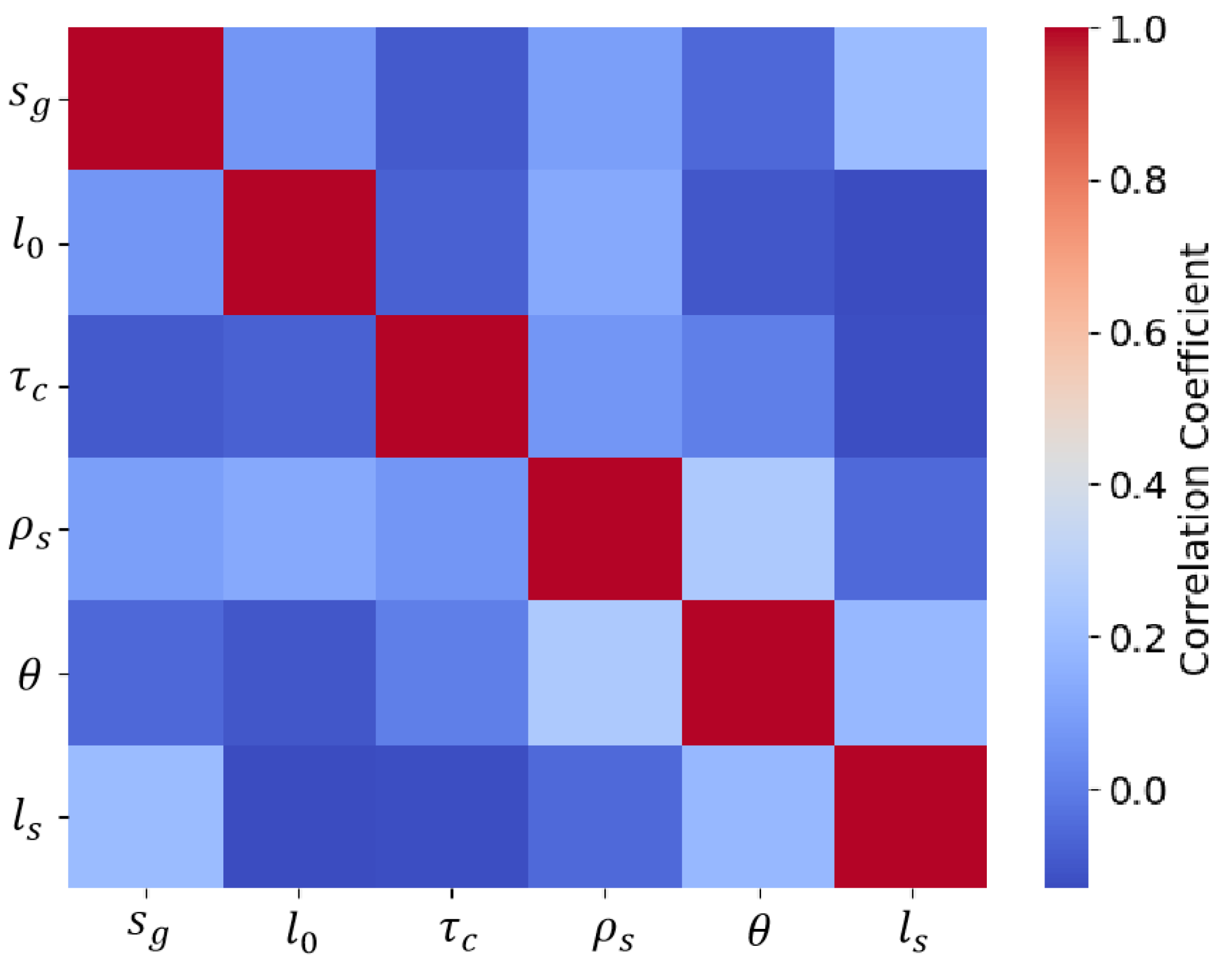
4.2. Parameters Selection

In this theoretical model, the explanatory variables include the yield stress ${\tau }_c$, consistency $\mu$, power-law index n, length of the material at the source area $l_0$, depth of the material at the gate $s_g$, distance between the gate and the indicated position $l_s$, slope angle $\theta$, density of the material ${\rho }_s$, time t, and gravity acceleration g. The explained variables include the depth s and the depth-averaged velocity u at different positions. See Figure 1 and Figure 2 for the physical reflections of $l_0,s_g,l_s,$ and $\theta$. The relation between explanatory and explained variables can be simplified using a $\eta (·)$ function, that is,

$$(s(\widehat{x},t),u(\widehat{x},t))=\eta ({\tau }_c,\mu ,n,l_0,s_g,l_s,\theta ,{\rho }_s,t,g)$$

(32)

The dynamic of the material moving along the slope strongly depends on its rheological characteristics, whose parameters include the yield stress ${\tau }_c$, consistency $\mu$, and power-law index n. Figure 8 presents a three-phase diagram illustrating the correlations among these three rheological parameters. These three parameters exhibit strong interdependencies with the correlation coefficients larger than 0.9. Given the pronounced correlations observed, yield stress ${\tau }_c$ can be effectively chosen as a representative parameter to characterize the rheological properties of debris flow materials. This selection simplifies the analysis and modeling of debris flow behavior, and reduces the complexity associated with considering multiple rheological variables simultaneously.

In addition, the objective of the model is to determine the frontal depth $s_0$ and frontal depth averaged velocity $u_0$ at $\widehat{x}$ = $l_s$, $\widehat{t}$ = $\Delta t$. In this case, time $\widehat{t}$ depends on the initial settings.

Table 3. The input and output parameters adopted for developing the SVR model.

Type	Parameters	Symbols
Input parameters	yield stress of the slide material	${\tau }_c$
	density of the slide material	${\rho }_s$
	depth of the material at the gate	$s_g$
	length of the material at the source area	$l_0$
	slope angle	$\theta$
	distance between the gate and indicated position	$l_s$
	depth of the slide on impact	$s_0$
Output parameters	depth-averaged velocity on impact	$u_0$

illustrates the input and output parameters adopted for SVR.

The input parameters are expected to be independent. To verify this, we analyzed the correlations among the input parameters used in numerical simulations. Figure 9 shows a heatmap representing the correlation coefficients between various variables labeled as $s_g$, $l_0$, ${\tau }_c$, ${\rho }_s$, $\theta$, and $l_s$. The x-axis and y-axis contain these variables. The color bar on the right side of the heatmap indicates the magnitude of the correlation, with the gradient ranging from blue to red. As observed in the figure, the correlation coefficients among most of the input parameters are relatively low, suggesting minimal interdependence. This supports the assumption that the input parameters can be treated as independent in the SVR modeling. The visualization effectively confirms that there is no significant multicollinearity among the variables, validating their use as independent parameters.

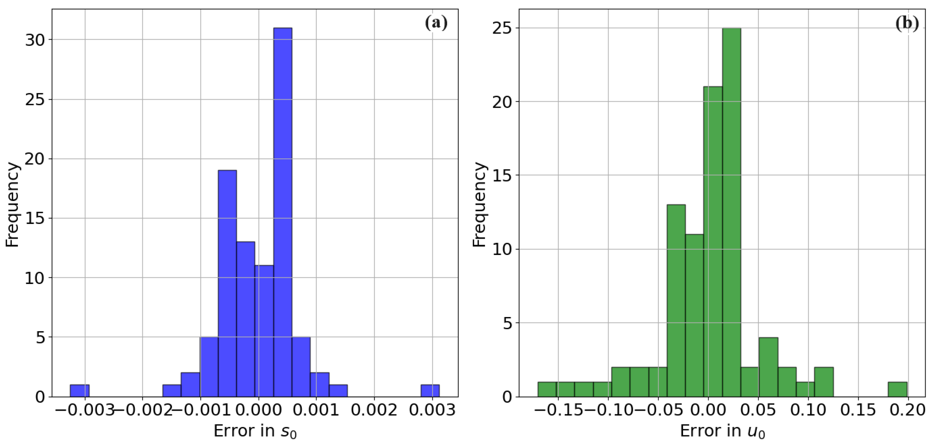
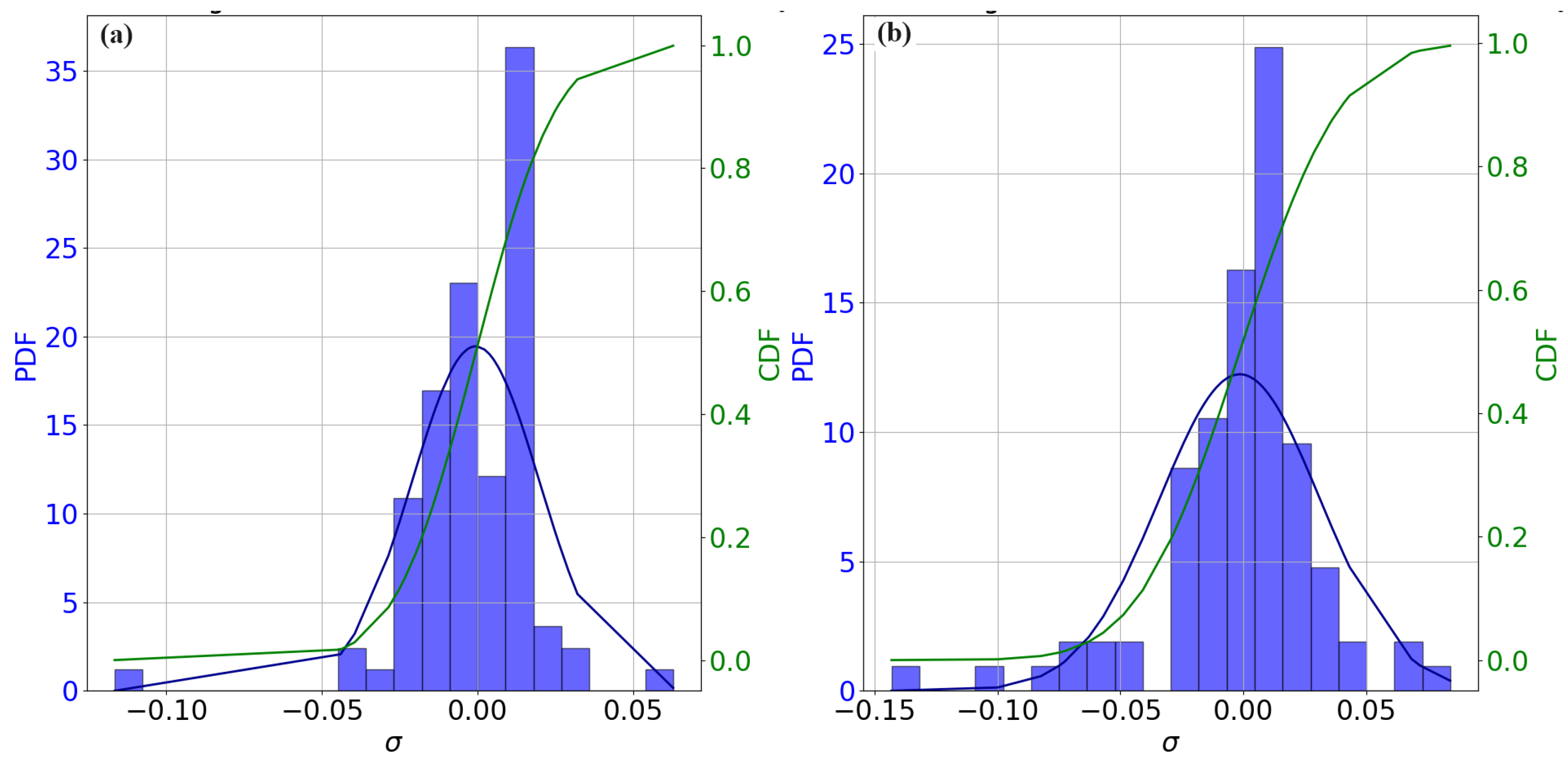
4.3. Regression Analysis Using the SVR Model

Figure 10 illustrates the modeling process of the SVR prediction, showing the sequence of steps involved in the SVR modeling process, highlighting the split between training and testing, the role of hyperparameters in training, and the flow from input to output through the trained model. The process begins with the input parameters (i.e., $s_g$, $l_0$, ${\tau }_c$, ${\rho }_s$, $\theta$, and $l_s$), which are split into two parts: 90% for the training dataset and 10% for the testing dataset. The training data are used to train the SVR model, where hyperparameters C and $ϵ$ are specified to optimize the model’s performance, where C controls the trade-off between maximizing the margin and minimizing the classification error, and $ϵ$ defines the margin of tolerance where no penalty is given to errors. After training, the model is then tested using the previously set-aside testing data. Finally, the model produces the output (i.e., $s_0$, $u_0$) based on the input data.

Figure 11 exhibits the performance of the predictive model by comparing the original and predicted values for the variables $s_0$ and $u_0$ in subplots (a) and (b), respectively. The blue scatter points, representing the training data, are closely aligned with the dashed 1:1 line in both subplots, indicating that the model performs well on the training dataset with minimal deviations between the predicted and actual values. The red scatter points, representing the testing data, generally align well with the 1:1 line, although some deviations are observed, as indicated by the error bars. These deviations suggest that while the model maintains strong predictive accuracy on unseen data, there are instances where the predictions diverge from the actual values. The original $s_0$ values range from approximately 0.025 to 0.050, while $u_0$ values range from 1.2 to 2.4, with the predicted values closely aligning with these ranges, demonstrating the model’s ability to accurately replicate the observed data across the full range of both variables. Overall, the proximity of the scatter points to the 1:1 line across both the training and testing datasets demonstrates the model’s effective generalization and predictive capability, though with some minor errors consistent with typical model behavior on new data.

The performance of the proposed model was evaluated by the relative residual $\sigma$ and coefficient of determination ($R^2$), which are expressed as follows:

$$\sigma ={\displaystyle \frac{\left(y_{p,i}-y_{o,i}\right)}{y_{o,i}}}$$

(33)

$$R^2=1-{\displaystyle \sum _{i=1}^{ϵ}}\left({\displaystyle \frac{{\left(y_{p,i}-y_{o,i}\right)}^2}{{\left(y_{p,i}-{\overline{y}}_{o,i}\right)}^2}}\right)$$

(34)

where $y_{p,i}$ are the predicted data, and $y_{o,i}$ are the observed data. The coefficient of determination $R^2$ for $s_0$ and $u_0$ is 0.956 and 0.911, respectively. Higher $R^2$ values suggest that the model performs well in capturing the variability of the data. Once $R^2$ is larger than 0.9, the model can be validated.

Figure 12 illustrates histograms of the error distributions for the variables $s_0$ and $u_0$. Figure 12a shows the error distribution for $s_0$. The histogram, represented in blue, displays the frequency of errors across 20 bins. The errors are calculated as the difference between the predicted and actual values, capturing the overall performance of the model in predicting $s_0$. The x-axis represents the error magnitude, while the y-axis indicates the frequency of occurrence. Figure 12b shows the error distribution for $u_0$. The histogram, shown in green, similarly depicts the frequency of errors. The axes are labeled consistently with the left subplot. For $s_0$, the errors are tightly clustered around 0, with most values ranging from $-0.002$ to $0.002$ and a peak near $0.001$, indicating that the model slightly overestimates the actual values in most cases. Few errors exceed $\pm 0.003$, highlighting the precision of the predictions. In contrast, the error distribution for $u_0$ is slightly wider, ranging from approximately $-0.10$ to $0.15$, with most errors concentrated between $-0.05$ and $0.05$ and a clear peak near 0. While some outliers are observed at the extremes (up to $0.20$), they are relatively rare. Overall, the error distributions demonstrate that the model performs well in predicting both $s_0$ and $u_0$, with the majority of errors being small and centered around zero, indicating strong accuracy and reliability.

The probability density distribution function (PDF) and cumulative distribution function (CDF) are then analyzed for both $\sigma$. The PDF curve serves as a theoretical model of the residual distribution, providing a benchmark against which the actual distribution can be assessed. The CDF is an essential tool for understanding the cumulative probability associated with the residuals up to any given value. By examining the CDF, one can determine the proportion of residuals that lie below a specific threshold, offering insight into the likelihood of encountering certain residual values. This cumulative perspective is particularly useful in assessing the overall performance of a predictive model, as it highlights the range of residuals and their probabilities.

Figure 13 illustrates the PDF and CDF of the relative residuals $\sigma$ for $s_0$ and $u_0$. The histograms in each subplot effectively summarize the distribution of the relative residuals, visually representing how frequently each residual value occurs and the spread and central tendency of the residuals. Superimposed on these histograms is a smooth PDF curve (dark blue), which is calculated based on the mean and standard deviation of the residuals. The divergence of the histogram from this PDF curve reveals how closely the residuals follow a normal distribution, which can be an important consideration in model validation and error analysis. The green line in each subplot represents the CDF of the relative residuals. For $s_0$, the PDF shows a symmetrical bell-shaped distribution centered around 0, with most errors ranging from $-0.02$ to $0.02$, and a steep rise in the CDF within this range indicates that the majority of errors are small, reaching a cumulative probability of nearly 1.0 by $\pm 0.05$. Similarly, the PDF for $u_0$ also displays a symmetrical distribution centered around 0, but with a slightly broader range of errors, extending from approximately $-0.05$ to $0.05$. The CDF for $u_0$ shows that most errors are concentrated within this range, with the cumulative probability approaching 1.0 by $\pm 0.10$. These distributions highlight that the model predicts both $s_0$ and $u_0$ with high accuracy, as errors are small and symmetrically distributed, though $u_0$ exhibits a slightly larger variability compared to $s_0$. The combined analysis of the PDF and CDF allows for a deeper understanding of the model’s accuracy and reliability, offering both a snapshot of residual frequency and a cumulative assessment of residual distribution.

5. Discussion

The current study presents a significant advancement in the prediction of debris flow dynamics by integrating viscoplastic theory with support vector regression (SVR) models. Traditional models often struggled to capture the complex, nonlinear behaviors inherent in debris flows; our proposed model, which combined theoretical and data-driven approaches, effectively addresses this challenge. Our theoretical framework, based on the Herschel–Bulkley model and incorporating the kinematic wave model and lubrication theory, provides a robust description of the mechanical physics governing debris flows. This model’s ability to generate extensive and detailed datasets has proven instrumental in training the SVR model, leading to high prediction accuracy. The integration of these methods bridges the gap between purely empirical models and those grounded in physical theory, offering a more comprehensive tool for debris flow prediction.

The findings indicate that our model can predict the key dynamics of debris flows, including flow velocity and depth, with high precision. This has significant implications for early warning systems and mitigation strategies. One key advantage of the proposed model is its ability to decrease the difficulty of debris flow prediction. Traditional theoretical models are often too complex for practical engineering applications. In contrast, the proposed method can generate massive numerical simulations in advance, building a comprehensive database. Training the factors recorded in this database using machine learning techniques not only captures the nonlinear relationships inherent in debris flows but also simplifies the prediction model, making it more accessible and easier to use in practical engineering contexts. Furthermore, the study underscores the importance of considering both viscous and plastic behaviors in understanding debris flow dynamics. Previous models often simplified these aspects, leading to less accurate predictions. Our approach, which incorporates the complexities of these behaviors, demonstrates the necessity of a detailed rheological analysis in predictive modeling.

However, while the method demonstrates good performance in simulated and controlled scenarios, its real-world applicability and accuracy have yet to be fully validated. The reliance on numerical simulations, although offering flexibility and the ability to explore various scenarios, may not fully capture the complexities and variability of real-world conditions. Considering the difficulty of recording real world debris flow events, one possible solution is to conduct physical model experiments to mimic real debris flows. The ideal approach would involve conducting physical model experiments and developing the regression model using experimental data. This would provide a more accurate and reliable dataset. The challenge, however, lies in finding ideal materials to generate a regularized dataset. Real-world materials often vary significantly, making it difficult to create consistent and representative experimental conditions.

It should be noted that the proposed model is confined to simulating mudflow-like debris flows, representing only a subset of all possible debris flow scenarios. This focus arises from the underlying assumptions based on the Herschel–Bulkley rheological model and lubrication theory, which are most applicable to such flow conditions. Debris flows occurring in heterogeneous geological conditions may exhibit behaviors that necessitate additional model modifications or alternative modeling approaches. Future work will aim to extend the current framework to encompass a broader range of debris flow phenomena, including those on steeper gradients and within more complex terrains.

In addition, the scarcity of comprehensive data on debris flow events, particularly those occurring in complex terrains, poses significant challenges for validating and refining predictive models. This limitation underscores the need for cautious interpretation of the model’s predictions and highlights areas where further empirical data collection is essential. Given the intricate interplay between terrain complexity and meteorological factors in real-world debris flows, future investigations will focus on integrating additional parameters into the model to better capture these dynamics. This includes incorporating topographical variability and climate-driven factors that influence debris flow initiation and progression.

6. Conclusions

This study demonstrates a novel approach to predicting debris flow dynamics by combining viscoplastic theory and machine learning methods. For the theoretical part, we consider the debris flow as a viscoplastic fluid whose rheological behavior follows the Herschel–Bulkley model. By integrating the lubrication model and the kinematic wave model, we seek to capture the essential physical mechanisms driving debris flow dynamics and determine the dominating factors governing the physical process. The numerical solution of the theoretical framework is used to generate an extensive training dataset, which is then employed to train the SVR model.

The proposed model demonstrated remarkable predictive performance, achieving coefficients of determination $R^2$ of 0.956 for slide depth and 0.911 for slide velocity on impact. Additionally, the relative residuals $\sigma$ for both slide depth and slide velocity were predominantly distributed within the narrow range of −0.05 to 0.05, indicating high accuracy and reliability in the predictions. These results underscore the efficacy of the hybrid modeling approach, which seamlessly integrates physical mechanisms with machine learning techniques to enhance predictive capabilities. The incorporation of key explanatory variables—yield stress, material density, source area depth and length, and slope length—proved crucial in refining the model’s accuracy. The high $R^2$ values and favorable residual distributions not only validate the model’s performance but also highlight its potential applicability in real-world scenarios. In addition, the ability to create a large database of numerical simulations and train machine learning models on this data allows for capturing nonlinear relationships and simplifying the overall prediction model.

Further studies should focus on expanding the model’s parameters and testing its efficacy in diverse environments. For instance, while our model incorporates various critical factors, additional variables such as weather patterns, vegetation cover, and human activity could further refine predictions. Moreover, the application of our model to different geographic regions with varying topographies and climatic conditions would test its robustness and adaptability.

References

1. Meng, Z. Experimental study on impulse waves generated by a viscoplastic material at laboratory scale. Landslides 2018, 15, 1173–1182. [Google Scholar] [CrossRef]
2. Meng, Z.; Zhang, J.; Hu, Y.; Ancey, C. Temporal Prediction of Landslide-Generated Waves Using a Theoretical-Statistical Combined Method. J. Mar. Sci. Eng. 2023, 11, 1151. [Google Scholar] [CrossRef]
3. Li, Y.; Cui, Y.; Hu, X.; Lu, Z.; Guo, J.; Wang, Y.; Wang, H.; Wang, S.; Zhou, X. Glacier retreat in Eastern Himalaya drives catastrophic glacier hazard chain. Geophys. Res. Lett. 2024, 51, e2024GL108202. [Google Scholar] [CrossRef]
4. Zhang, J.; Zhang, X.; Li, H.; Fan, Y.; Meng, Z.; Liu, D.; Pan, S. Optimization of Water Quantity Allocation in Multi-Source Urban Water Supply Systems Using Graph Theory. Water 2024, 17, 61. [Google Scholar] [CrossRef]
5. Chen, H.; Huang, S.; Xu, Y.P.; Teegavarapu, R.S.; Guo, Y.; Nie, H.; Xie, H. Using baseflow ensembles for hydrologic hysteresis characterization in humid basins of Southeastern China. Water Resour. Res. 2024, 60, e2023WR036195. [Google Scholar] [CrossRef]
6. Coussot, P.; Laigle, D.; Arattano, M.; Deganutti, A.; Marchi, L. Direct determination of rheological characteristics of debris flow. J. Hydraul. Eng. 1998, 124, 865–868. [Google Scholar] [CrossRef]
7. Hutter, K.; Svendsen, B.; Rickenmann, D. Debris flow modeling: A review. Contin. Mech. Thermodyn. 1994, 8, 1–35. [Google Scholar] [CrossRef]
8. Zhou, W.; Qiu, H.; Wang, L.; Pei, Y.; Tang, B.; Ma, S.; Yang, D.; Cao, M. Combining rainfall-induced shallow landslides and subsequent debris flows for hazard chain prediction. Catena 2022, 213, 106199. [Google Scholar] [CrossRef]
9. Takahashi, T. Debris Flow: Mechanics, Prediction and Countermeasures; CRC Press: Boca Raton, FL, USA, 2003. [Google Scholar]
10. Ma, T.; Chen, H.; Zhang, K.; Shen, L.; Sun, H. The rheological intelligent constitutive model of debris flow: A new paradigm for integrating mechanics mechanisms with data-driven approaches by combining data mapping and deep learning. Expert Syst. Appl. 2025, 126405. [Google Scholar] [CrossRef]
11. Zegers, G.; Mendoza, P.A.; Garces, A.; Montserrat, S. Sensitivity and identifiability of rheological parameters in debris flow modeling. Nat. Hazards Earth Syst. Sci. 2020, 20, 1919–1930. [Google Scholar] [CrossRef]
12. Petley, D.N.; Bulmer, M.H.; Murphy, W. Patterns of movement in rotational and translational landslides. Geology 2002, 30, 719–722. [Google Scholar] [CrossRef]
13. Van Westen, C.J.; Castellanos, E.; Kuriakose, S.L. Spatial data for landslide susceptibility, hazard, and vulnerability assessment: An overview. Eng. Geol. 2008, 102, 112–131. [Google Scholar] [CrossRef]
14. Tien Bui, D.; Tuan, T.A.; Klempe, H.; Pradhan, B.; Revhaug, I. Spatial prediction models for shallow landslide hazards: A comparative assessment of the efficacy of support vector machines, artificial neural networks, logistic regression, and their ensemble. Geomorphology 2016, 231, 102–120. [Google Scholar]
15. Meng, Z.; Hu, Y.; Ancey, C. Using a data driven approach to predict waves generated by gravity driven mass flows. Water 2020, 12, 600. [Google Scholar] [CrossRef]
16. Cui, Y.; Li, Y.; Tang, H.; Turowski, J.M.; Yan, Y.; Bazai, N.A.; Wei, R.; Li, L. A digital-twin platform for cryospheric disaster warning. Natl. Sci. Rev. 2024, 11, nwae300. [Google Scholar] [CrossRef]
17. Chmiel, M.; Walter, F.; Wenner, M.; Zhang, Z.; McArdell, B.W.; Hibert, C. Machine learning improves debris flow warning. Geophys. Res. Lett. 2021, 48, e2020GL090874. [Google Scholar] [CrossRef]
18. Huang, J.; Hales, T.C.; Huang, R.; Ju, N.; Li, Q.; Huang, Y. A hybrid machine-learning model to estimate potential debris-flow volumes. Geomorphology 2020, 367, 107333. [Google Scholar] [CrossRef]
19. Korup, O.; Stolle, A. Landslide prediction from machine learning. Geol. Today 2014, 30, 26–33. [Google Scholar] [CrossRef]
20. Pradhan, B.; Lee, S. Landslide susceptibility assessment and factor effect analysis: Backpropagation artificial neural networks and their comparison with frequency ratio and bivariate logistic regression modelling. Environ. Model. Softw. 2010, 25, 747–759. [Google Scholar] [CrossRef]
21. Wang, L.J.; Guo, M.; Sawada, K.; Lin, J.; Zhang, J. A comparative study of landslide susceptibility maps using logistic regression, frequency ratio, decision tree, weights of evidence and artificial neural network. Geosci. J. 2016, 20, 117–136. [Google Scholar] [CrossRef]
22. Chen, H.; Xu, B.; Qiu, H.; Huang, S.; Teegavarapu, R.S.; Xu, Y.P.; Guo, Y.; Nie, H.; Xie, H. Adaptive assessment of reservoir scheduling to hydrometeorological comprehensive dry and wet condition evolution in a multi-reservoir region of southeastern China. J. Hydrol. 2025, 648, 132392. [Google Scholar] [CrossRef]
23. Huangfu, W.; Qiu, H.; Cui, P.; Yang, D.; Liu, Y.; Tang, B.; Liu, Z.; Ullah, M. Quick and automatic detection of co-seismic landslides with multi-feature deep learning model. Sci. China Earth Sci. 2024, 67, 2311–2325. [Google Scholar] [CrossRef]
24. Wei, Y.; Qiu, H.; Liu, Z.; Huangfu, W.; Zhu, Y.; Liu, Y.; Yang, D.; Kamp, U. Refined and dynamic susceptibility assessment of landslides using InSAR and machine learning models. Geosci. Front. 2024, 15, 101890. [Google Scholar] [CrossRef]
25. Liu, Z.; Qiu, H.; Zhu, Y.; Huangfu, W.; Ye, B.; Wei, Y.; Tang, B.; Kamp, U. Increasing irrigation-triggered landslide activity caused by intensive farming in deserts on three continents. Int. J. Appl. Earth Obs. Geoinf. 2024, 134, 104242. [Google Scholar] [CrossRef]
26. Stumpf, A.; Malet, J.P.; Kerle, N.; Niethammer, U.; Rothmund, S. Image-based mapping of surface fissures for the investigation of landslide dynamics. Geomorphology 2018, 231, 102–113. [Google Scholar] [CrossRef]
27. Meng, Z.; Wang, Y.; Zheng, S.; Wang, X.; Liu, D.; Zhang, J.; Shao, Y. Abnormal Monitoring Data Detection Based on Matrix Manipulation and the Cuckoo Search Algorithm. Mathematics 2024, 12, 1345. [Google Scholar] [CrossRef]
28. Ancey, C.; Cochard, S. The dam-break problem for Herschel–Bulkley viscoplastic fluids down steep flumes. J. -Non-Newton. Fluid Mech. 2009, 158, 18–35. [Google Scholar] [CrossRef]
29. Ancey, C.; Andreini, N.; Epely-Chauvin, G. Viscoplastic dambreak waves: Review of simple computational approaches and comparison with experiments. Adv. Water Resour. 2012, 48, 79–91. [Google Scholar] [CrossRef]
30. Meng, Z.; Ancey, C. The effects of slide cohesion on impulse-wave formation. Exp. Fluids 2019, 60, 151. [Google Scholar] [CrossRef]
31. Meng, Z.; Li, X.; Han, S.; Wang, X.; Meng, J.; Li, Z. The Motion and Deformation of Viscoplastic Slide while Entering a Body of Water. J. Mar. Sci. Eng. 2022, 10, 778. [Google Scholar] [CrossRef]
32. Meng, Z.; Hu, J.; Zhang, J.; Zhang, L.; Yuan, Z. The Momentum Transfer Mechanism of a Landslide Intruding a Body of Water. Sustainability 2023, 15, 13940. [Google Scholar] [CrossRef]
33. Suthaharan, S.; Suthaharan, S. Support vector machine. In Machine Learning Models and Algorithms for Big Data Classification: Thinking with Examples for Effective Learning; Springer Nature: Berlin, Germany, 2016; pp. 207–235. [Google Scholar]
34. Pisner, D.A.; Schnyer, D.M. Support vector machine. In Machine learning; Elsevier: Amsterdam, The Netherlands, 2020; pp. 101–121. [Google Scholar]
35. Chang, C.C.; Lin, C.J. LIBSVM: A library for support vector machines. ACM Trans. Intell. Syst. Technol. (TIST) 2011, 2, 1–27. [Google Scholar] [CrossRef]
36. Singh, A.; Kotiyal, V.; Sharma, S.; Nagar, J.; Lee, C.C. A machine learning approach to predict the average localization error with applications to wireless sensor networks. IEEE Access 2020, 8, 208253–208263. [Google Scholar] [CrossRef]
Figure 1. The simplified physical model of the issue: (a) schematic diagram and (b) physical model.
Water 17 00120 g001
Figure 2. Sketch of the sliding mass (a) at rest and (b) moving along the slope.
Water 17 00120 g002
Figure 3. The flowchart of the SVR model.
Water 17 00120 g003
Figure 4. The structure of SVR [36].
Water 17 00120 g004
Figure 5. Numerical solution of slide thickness s ( x ^ , t ) along the chute of the example case.
Water 17 00120 g005
Figure 6. Numerical solution of depth-averaged velocity u ( x ^ , t ) along the chute of the example case.
Water 17 00120 g006
Figure 7. Time variation of (a) slide thickness s ( t ) and (b) depth-averaged velocity u ( t ) at an indicated position l s = 0.95 with various initial settings.
Water 17 00120 g007
Figure 8. Three-phase diagram of the rheological parameters yield stress τ c , consistency μ , and power-law index n.
Water 17 00120 g008
Figure 9. The correlations among the selected input parameters.
Water 17 00120 g009
Figure 10. The modeling process of the SVR prediction.
Water 17 00120 g010
Figure 11. Comparision of the predicted and original (a) s 0 and (b) u 0 .
Water 17 00120 g011
Figure 12. The error histogram distribution of the (a) s 0 and (b) u 0 .
Water 17 00120 g012
Figure 13. The PDF and CDF of σ for (a) s 0 and (b) u 0 .
Water 17 00120 g013