Reducing Water Conveyance Footprint through an Advanced Optimization Framework

Abstract

This study investigates the optimal and safe operation of pumping stations in water distribution systems (WDSs) with the aim of reducing the environmental footprint of water conveyance processes. We introduced the nonlinear chaotic honey badger algorithm (NCHBA), a novel and robust optimization method. The proposed method utilizes chaotic maps to enhance exploration and convergence speed, incorporating a nonlinear control parameter to effectively balance local and global search dynamics. Single-objective optimization results on a WDS show that NCHBA outperforms other algorithms in solution accuracy and convergence speed. The application of the proposed approach on a water network with two variable-speed pumps demonstrated a significant 27% reduction in energy consumption. Expanding our focus to the multi-objective optimization of pump scheduling programs in large-scale water distribution systems (WDSs), we employ the non-dominated sorting nonlinear chaotic honey badger algorithm (MONCHBA). The findings reveal that the use of variable-speed pumps not only enhances energy efficiency but also bolsters WDS reliability compared to the use of single-speed pumps. The results showcase the potential and robustness of the proposed multi-objective NCHBA in achieving an optimal Pareto front that effectively balances energy consumption, pressure levels, and water quality risk, facilitating carbon footprint reduction and sustainable management of WDSs.

1. Introduction

One of the main essential infrastructures of every urban area is the water distribution system (WDS), which delivers water of sufficient quality and quantity to consumers [1]. Pumping stations (PSs) are one of the most expensive parts of a WDS and have the most crucial role in supplying water with the proper pressure in the network, so their proper design and use are critical. Pumping an excess amount of water into the network increases energy consumption by raising the nodal pressure beyond the necessary pressure in the nodes, causing leaks, broken pipes, and, as a result, increasing the maintenance costs of the water distribution system [2]. On the other hand, if the pumping stations do not supply enough water to the consumers during the peak hours of the day and night, the network’s reliability will decrease [3]. One of the ways to increase the reliability and flexibility of the water supply network is by using more than one pump in the pumping stations. The number of pumps can be determined by a simple economic analysis. Based on the financial reports of England and Wales between 1998 and 1999, the cost of electricity used by pumping stations was estimated to be more than GBP 120 million [4]. Therefore, in addition to adequately designing pumping stations, it is necessary to use them properly. The problem of optimal operation of pumping stations is an important issue influenced by several factors, such as the following: B. the performance of the pump and the time of pumping. In the last decades, much research has been conducted on optimizing the performance of pumps, using various optimization approaches such as linear programming (LP), nonlinear programming (NLP), and dynamic programming (DP) [5,6,7,8,9]. The above computational approaches are time-consuming and unsuitable for estimating the optimal operation of pumping stations due to many decision variables impacting the optimization of pumping stations [10]. Therefore, in recent years, researchers have focused on meta-heuristics approaches to optimize these systems [11,12,13,14,15,16,17,18,19]. Among the existing studies, ref. [20] introduced a new simulation–optimization model for optimizing the pump scheduling program by using an Ant Colony Optimization (ACO). In this study, an explicit method is presented to reduce the decision variables and to satisfy the constraint of pump switching. More recently, ref. [21] developed a new simulation–optimization model based on an improved Dragonfly Algorithm (DA) to optimize the scheduling of pumping stations and minimize energy consumption in WDSs. Comparing the performance of the proposed model with previous models in a famous case study, the result illustrated that the DA-based model was more efficient and more reliable than others.

In recent years, the problem of optimizing the operation of pumping stations has been extensively studied to simulate it as a multi-purpose problem because it involves various conflicting objectives [22,23,24]. The most noteworthy studies in the last few years include ref. [25], who proposed a self-adaptive multi-objective optimization algorithm based on the Non-Dominated Sorting Genetic Algorithm (NSGA-II) for optimizing the pump scheduling program with the objective functions of 1—energy consumption cost and 2—the maintenance cost. Ref. [26] introduced a new framework using the NSGA-II for determining the best program of pumping in order to reduce the energy and leakage in WDSs. As such, in operating pumping stations, many objectives, such as minimizing leakage, energy costs, and water age, are to be considered. This is performed through multi-objective optimization models [27,28,29,30] and is the main motivation for this study.

The multi-objective optimization problem of the operation of pumping stations in WDSs is one of the most challenging problems in the field of water engineering. Typically, this problem includes nonlinear objective functions with a large number of decision variables and constraints. Water managers and planners explore to find proper optimization techniques for the optimal operation of pumping stations. Therefore, finding robust and efficient optimization methods is essential. Meta-heuristic algorithms are proposed as the most frequently implemented methods for optimizing pump scheduling programs in WDSs regarding their proven powerful ability to find non-dominated optimal solution sets and convergence speed [25]. Simple design and implementation, high performance, and robustness are the superior characteristics of these techniques [30,31,32,33].

Therefore, this study aims to develop an effective and new optimization algorithm for the operation of pumping stations, taking into consideration multiple objectives. To achieve this, we enhanced the performance of a meta-heuristic optimization algorithm known as the honey badger algorithm (HBA) [34] by improving its search capabilities in the solution space and facilitating suitable convergence. The proposed algorithm’s performance is evaluated on both small-scale WDSs with variable-speed pumps and large-scale WDSs. Two scenarios, including variable-speed and fixed-speed pumps, are considered, with the overall objective of ensuring optimal and safe operation of pumping stations. The key novel contributions of this study are summarized as follows:

• A nonlinear chaotic honey badger algorithm, i.e., NCHBA, incorporating a nonlinear control parameter and a chaotic map to strike a balance between exploration and exploitation, is proposed. The efficiency of NCHBA is validated by solving a high-dimensional pump scheduling problem.
• A new multi-objective variant of NCHBA is proposed, and its performance is assessed using four ZDT benchmark functions.
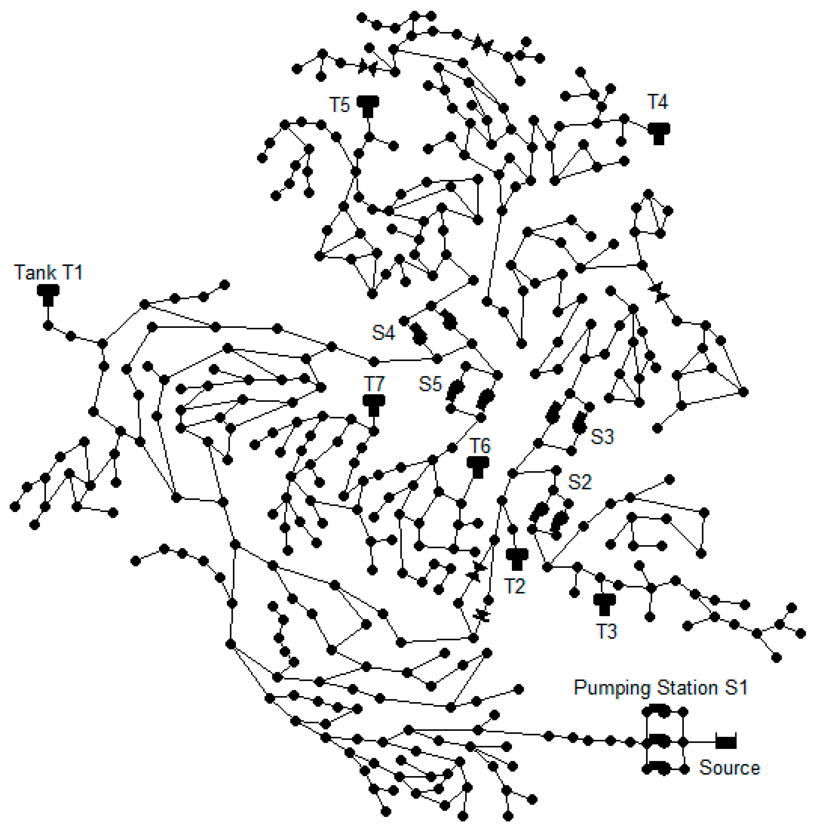
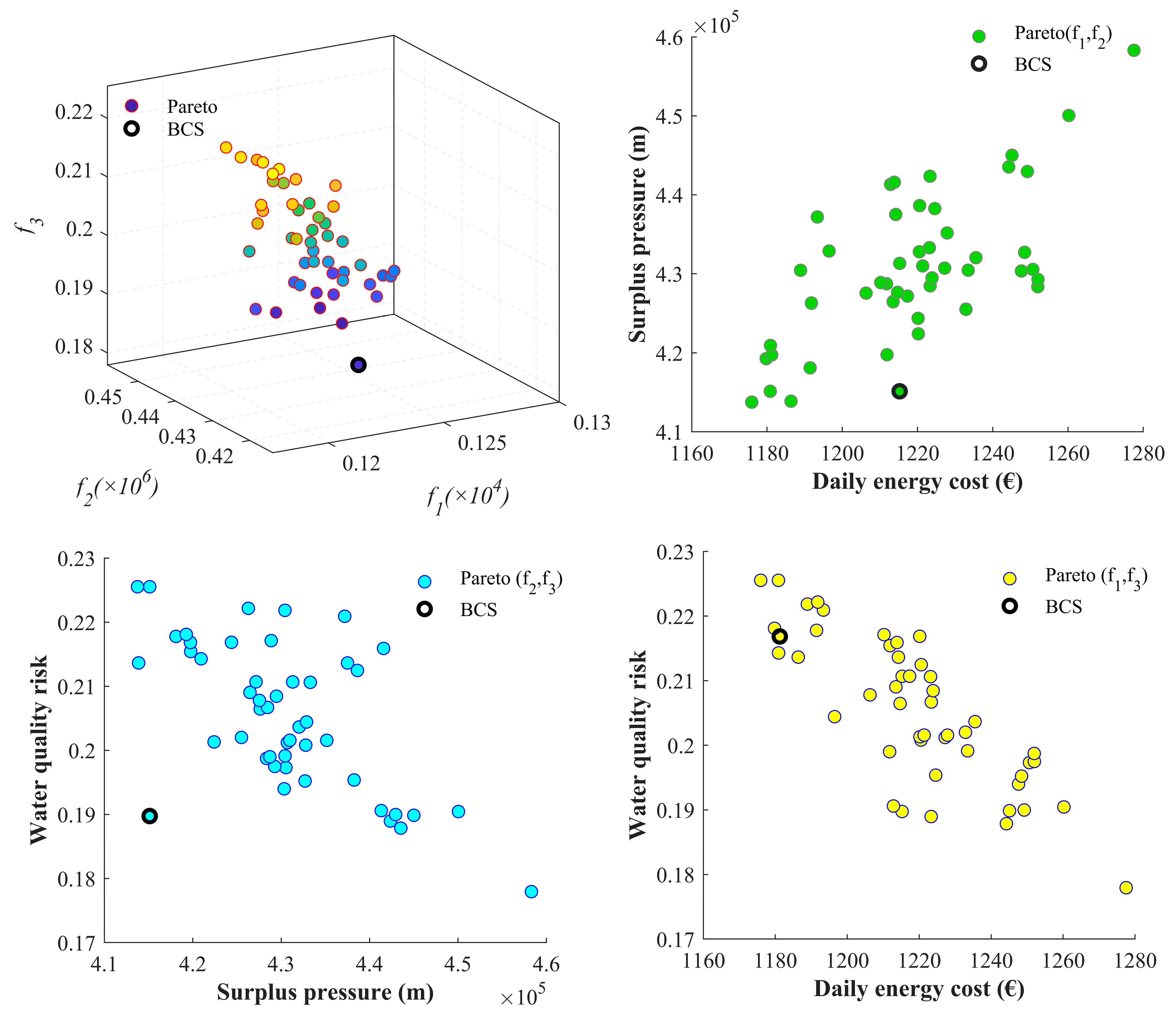
• The proposed multi-objective algorithm is utilized to optimize the pump scheduling program of a large WDS to minimize the energy consumption and footprint of pumping stations, quality risk, and nodal pressure. The optimal compromise solution is determined through the TOPSIS method.

The structure of the rest of this paper is as follows: Section 2 provides a detailed description of the model development. Section 3 showcases the results of the proposed algorithm for optimizing the pump scheduling program. Section 4 discusses the key conclusions of the study and directions for future research.

2. Materials and Methods

This section provides an overview of the necessary materials and methods for developing the proposed multi-objective framework aimed at achieving sustainable and optimized operation of WDSs. It includes a description of the fundamental HBA and its framework, as well as an explanation of the key concepts related to the caostica map and nonlinear approach. Additionally, the information on the case studies and objective functions utilized in this study are presented in this section.

To find the best operating program for pumps in WDSs, a simulation optimization model was developed. To this end, the EPANET hydraulic simulation model [35] was coupled with the new proposed multi-objective optimization algorithm, i.e., MONCHBA, to achieve an enhanced and optimized operational model. Figure 1 illustrates the step-wise simulation–optimization processes of the proposed framework.

As depicted in Figure 1, the optimizer generates a vector of decision variables such as a scheduling program or operating cycle of pumps. Subsequently, the EPANET simulator model is executed, and the network’s response, including objective functions and constraints, is determined based on the input vector. This iterative process continues until the termination condition is met.

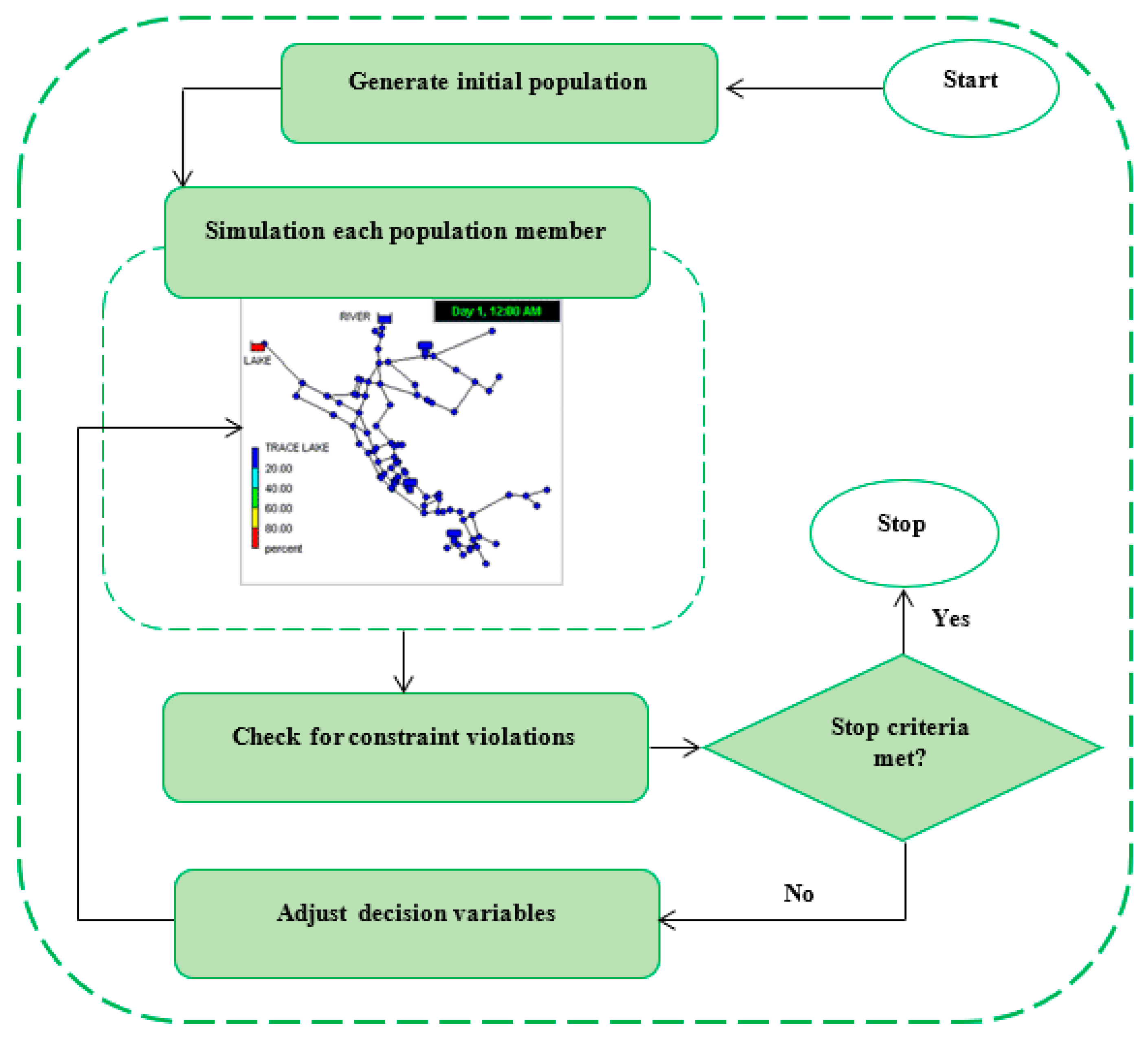
2.1. Optimization Process and Problem Formulation

This paper presents a new approach for optimized operation of pumps in water distribution systems. The proposed approach involves an explicit control optimization problem that considers the pumps’ operating times and relative speed as decision variables. This research explores pump energy efficiency across two scenarios with fixed and variable-speed pumps. Therefore, a multi-objective optimization approach is considered, where the purpose is to reduce the energy costs, pressure level, and water quality risk associated with the network operation. In this section, the formulation of the optimization problem is presented.

2.1.1. Objective Functions

The first objective function is the pumping energy cost (C_E), which includes two parts: demand charge (C_D) and consumption charge (Cc). Cc is the cost of electrical energy consumed during a time period. C_D denotes the demand charge, which is the total cost associated with the maximum amount of power consumed (i.e., peak energy). Therefore, the total pumping energy cost is computed by Equation (1) as follows [36]:

$$f_1=C_E=\stackrel{C_c}{\overbrace{{\gamma }_w{\displaystyle \sum }_{n=1}^{NP}{\displaystyle \sum }_{t=1}^T\left(\frac{Q_{\left(n,t\right)}.H_{\left(n,t\right)}}{{\eta }_{\left(n,t\right)}}\times ∆t_t\times b_{\left(n,t\right)}\times E{C}_{\left(n,t\right)}\right) }}+\stackrel{C_D}{\overbrace{{\displaystyle \sum }_{n=1}^{NP}\left(D{C}_n\times {\alpha }_n\right) }}$$

(1)

where $NP$ is the number of pumps, T is the number of time periods, ${\gamma }_w$ is the specific weight of water, $Q_{\left(n,t\right)} \mathrm{and} H_{\left(n,t\right)}$ are the flow through the pump and the total dynamic head during each time step t in pump n, $E{C}_{\left(n, t\right)}$ is the price per energy unit defined for each pump n according to the tariff value for the time step t, $b_{n,t}$ is the status of pump n as being off or on at time t, $∆t_t$ is the length of a time interval t, and ${\eta }_{\left(n,t\right)}$ is the efficiency of pump n during each time step t. To calculate the C_D, the model first finds the highest power required for each pump ($P_{max}$) throughout the simulation and counts how often it happens. Then, it multiplies this number by a user-defined demand charge ($D{C}_n$) for each pump. Therefore, ${\alpha }_n$ is the product of the maximum power for a pump $n$, $P_{max}$, and the frequency of this power, $n_{P_{max}}$, i.e.,

$${\alpha }_n=P_{max}\times n_{P_{max}}$$

(2)

The goal of minimizing energy consumption is to increase an approximate efficiency value. This is due to the fact that energy consumption depends on the scheduling program, the operating point, and the pump speed.

Operating a WDS with high pressure may lead to more leakages, pipe damage, and excessive consumption. In fact, a WDS is designed for a peak demand state; therefore, for long periods, it may tolerate excessive pressure, especially when the water consumption is low. Therefore, pressure management is an efficient way to improve the reliability of WDSs. Thus, we will consider the minimization of total excessive pressure of all nodes as our second objective function for optimal operation of the WDSs. The mathematical formulation of the second objective function can be defined as:

$$f_2={\displaystyle \sum }_{i=1}^N{\displaystyle \sum }_{t=1}^T{\left(P_{i,t}-P_i^{min}\right)}^2$$

(3)

where $P_{i,t}$ is the pressure at node i in time t, and $P_i^{min}$ is the minimum required pressure at node i.

The third objective function of the problem is to minimize the water quality risk in WDSs. It is clear that water quality deteriorates with increasing the water age. Applying some actions to increase the water quality in a network may lead to an increase in operational costs. Therefore, it is necessary for a sustainable WDS to acquire a reliable level of water age at which the water quality reliability is satisfied at the minimum operational costs. The mathematical formulation of water quality risk based on water age can be defined as Equation (4) [37]:

$$f_3=Ris{k}_q=1-R{e}_q$$

(4)

In Equation (5), $R{e}_q$ denotes the total water quality reliability of WDSs based on water age, determined as follows:

$$R{e}_q=\frac{{{\displaystyle \sum }}_{i=1}^N{{\displaystyle \sum }}_{t=1}^T{b}_{i,t}{Q}_{i,t}^{avl}}{{{\displaystyle \sum }}_{i=1}^N{{\displaystyle \sum }}_{t=1}^T{Q}_{i,t}^{req}}$$

(5)

where $b_{i,t}$ is a coefficient for node i at time t based on water age and is calculated from Equation (6), and $Q_{i,t}^{req}$ and $Q_{i,t}^{avl}$ are the required demand and the available discharge for node i at time t, respectively.

$$b=\{\begin{array}{cc}\hspace{1em}\hspace{1em}\hspace{1em}\hspace{1em}\hspace{1em}1\hfill & if water age \le 6\hfill \\ \hspace{1em}\hspace{1em}\hspace{1em}\hspace{1em}\hspace{1em}-0.125\times \left(WA-6\right)+1\hfill & if 6 \mathrm{h}<water age<10 \mathrm{h}\hfill \\ \hspace{1em}\hspace{1em}\hspace{1em}\hspace{1em}\hspace{1em}0\hfill & if 10 \mathrm{h}\le water age\hfill \end{array}$$

(6)

where $WA$ is the water age (hour), and b is the performance index. According to Equation (6), if the water age is less than 6 h, the performance of the network is good. If the water age is higher than 10 h, the performance of the network is poor.

It is worth noting that the available discharge at nodes is calculated here through the pressure-driven simulation method (PDSM). In this method, the discharge at each node depends on the nodal pressure. Many studies have suggested equations to simulate the relationship between the pressure and available discharge at the node [2]. The equation suggested by Wanger et al. (1988) for simulating the PDSM approach is used here [38]:

$$Q_{i,t}^{avl}(P_{i,t})=\{\begin{array}{cc}\hspace{1em}\hspace{1em}\hspace{1em}{Q}_{i,t}^{req}\hfill & P_{i,t}\ge P_i^{ref}\hfill \\ \hspace{1em}\hspace{1em}\hspace{1em}{Q}_{i,t}^{req}\times {\left(\frac{P_{i,t}-P_i^{min}}{P_i^{ref}-P_i^{min}}\right)}^{0.5}& P_i^{min}<P_{i,t}<P_i^{ref}\\ \hspace{1em}\hspace{1em}\hspace{1em}0\hfill & P_{i,t}\le P_i^{min}\end{array}$$

(7)

where $P_i^{ref}$ is the service pressure necessary for supplying the demand at nod i, $Q_{i,t}^{req}$ is the demand required at node i, and $P_i^{min}$ is the minimum pressure (which indicates no water is available at the node).

2.1.2. Constraints

Typically, several important constraints are applied to the operation optimization problem of WDSs to maintain the performance of the system. A constraint is implemented to maintain the balance between the water level of each tank at the beginning and at the end of the simulation duration, as demonstrated in Equation (8) [36]:

$${\mathrm{g}}_{1,i}=L_{i, final}-L_{i, initial}\le 0, i=1,\dots , n_{tanks}$$

(8)

where $L_{i, initial}$ and $L_{i, final}$ are the initial and final water levels of tank i, and $n_{tanks}$ is the number of existing tanks in a WDS. There are also two constraints that should be satisfied to control the water level variation in tanks between minimum and maximum allowable limits. These constraints are given as follows:

$${\mathrm{g}}_{2,i}=L_i-L_{i, max}\le 0, i=1,\dots , n_{tanks}$$

(9)

$${\mathrm{g}}_{3,i}=L_{i, min}-L_i\le 0, i=1,\dots , n_{tanks}$$

(10)

where $L_i$ is the water level in tank i, and $L_{i, max}$ and $L_{i, min}$ are the maximum and minimum limits in tank i, respectively.

To supply the required discharge at nodes, it is necessary that the pressure at the demand nodes should be higher than the minimum required pressure. Thus, another constraint is applied to the problem as follows:

$${\mathrm{g}}_{4,i}=P_i^{ref}-P_i\le 0, i=1,\dots , n_{nodes}$$

(11)

The fifth constraint relates to the deliverable flow by pumps that is a function of the pump characteristics, as shown in Equation (12):

$${\mathrm{g}}_{5,i}=Q_{\left(i,t\right)}-Q_i^{max}\le 0, i=1,\dots , n_{pumps}$$

(12)

where $Q_i^{max}$ is the maximum flowrate from the performance curve of pump i.

The last type of constraint includes the hydraulic compatibility equations of continuity and energy conservation, which are automatically satisfied in the EPANET hydraulic simulation model. More information on the compatibility restrictions is provided in Appendix A.

In brief, the multi-objective optimization model developed in this work can be mathematically expressed by Equation (13):

$$\begin{gathered} Min F_1=C_E\left(\mathit{X}\right)=\stackrel{C_c}{\overbrace{{\gamma }_w{\displaystyle \sum }_{n=1}^{NP}{\displaystyle \sum }_{t=1}^T\left(\frac{Q_{\left(n,t\right)}\left(\mathit{X}\right).H_{\left(n,t\right)}\left(\mathit{X}\right)}{{\eta }_{\left(n,t\right)}\left(\mathit{X}\right)}\times ∆t_t\times b_{\left(n,t\right)}\times E{C}_{\left(n,t\right)}\right) }}+\stackrel{C_D}{\overbrace{{\displaystyle \sum }_{n=1}^{NP}\left(D{C}_n\times {\alpha }_n\left(\mathit{X}\right)\right) }} \\ Min F_2={\displaystyle \sum }_{i=1}^N{\displaystyle \sum }_{t=1}^T{\left(P_{i,t}\left(\mathit{X}\right)-P_i^{ref}\right)}^2 \\ Min F_3=Ris{k}_q=1-\frac{{{\displaystyle \sum }}_{i=1}^N{{\displaystyle \sum }}_{t=1}^T{b}_{i,t}\left(\mathit{X}\right).Q_{i,t}^{avl}\left(\mathit{X}\right)}{{{\displaystyle \sum }}_{i=1}^N{{\displaystyle \sum }}_{t=1}^T{Q}_{i,t}^{req}} \\ \begin{array}{ccc}\mathrm{Subjected} \mathrm{to} :\hfill & {\mathrm{g}}_{1,i}\left(\mathit{X}\right)=L_{i,\mathit{final}}\left(\mathit{X}\right)-L_{i, initial}\left(\mathit{X}\right)\le 0,\hfill & i=1,\dots , n_{tanks}\hfill \\ & {\mathrm{g}}_{2,i}\left(\mathit{X}\right)=L_i\left(\mathit{X}\right)-L_{i, max}\le 0,\hfill & i=1,\dots , n_{tanks}\hfill \\ & {\mathrm{g}}_{3,i}\left(\mathit{X}\right)=L_{i, min}-L_i\left(\mathit{X}\right)\le 0,\hfill & i=1,\dots , n_{tanks}\\ & {\mathrm{g}}_{4,i}\left(\mathit{X}\right)=P_i^{ref}-P_i\left(\mathit{X}\right)\le 0,\hfill & i=1,\dots , n_{nodes}\\ & {\mathrm{g}}_{5,i}\left(\mathit{X}\right)=Q_{\left(i,t\right)}\left(\mathit{X}\right)-Q_i^{max}\le 0,\hfill & i=1,\dots , n_{pumps}\end{array} \end{gathered}$$

(13)

where $\mathit{X}=\left[\begin{array}{c}{x}_t^{Pump 1}\\ ⋮\\ x_t^{Pump n}\end{array} \begin{array}{c}\dots \\ ⋮\\ \dots \end{array} \begin{array}{c}{x}_T^{Pump 1}\\ ⋮\\ x_T^{Pump n}\end{array} \right]$ represents a vector of decision variables. The relative pump speed or the pump on/off status during the simulation period can be considered as the decision variables of the problem.

As previously mentioned, a new multi-objective optimization algorithm is proposed based on the nonlinearity and complexity of the problem. Honey badger algorithm (HBA) was improved and applied to optimize the objective functions. In the following subsections, a summary description of the proposed algorithm in this study is provided.

2.2. Optimization Model

2.2.1. Honey Badger Algorithm

The honey badger algorithm (HBA) is a newly nature-inspired algorithm proposed by Hashim et al. [34]. The HBA was mimicked from the honey badgers’ social behavior in exploring the food. The honey badger uses two ways to find food sources: smelling and digging or pursuing the honeyguide bird. Therefore, the basis of the HBA algorithm is these two modes. This algorithm consists of five main steps as follows:

Step 1: Initialization phase: Generate the randomly initial solutions (honey badgers’ positions) as follows:

$$x_i=L{B}_i+rand\times \left(U{B}_i-L{B}_i\right)$$

(14)

where $x_i$ explains the position of honey badger i, rand is a random number in [0, 1], and $L{B}_i$ and $U{B}_i$ are the lower and upper boundaries of the search space, respectively.

The initial random population of solutions is represented as:

$$\mathit{X}={\left[\begin{array}{ccc}{x}_{1,1}^1& \cdots & x_{1,D}^1\\ ⋮& \ddots & ⋮\\ x_{N,1}^1& \cdots & x_{N,D}^1\end{array}\right]}_{N\times D}$$

(15)

$$x_i=\left[x_i^1,x_i^2, \dots ,x_i^D\right]$$

(16)

where D and N are the number of decision variables and the number of honey badgers, respectively.

Step 2: Specifying intensity (I): To simulate the concentration strength of the prey and spacing between it and the ith hunter (honey badger), the intensity parameter ($\mathrm{I}$) is defined. In fact, ${\mathrm{I}}_{\mathrm{it}}$ explains the intensity of the smell of the prey; if the smell is heavy, the action will be quick and contrariwise. ${\mathrm{I}}_{\mathrm{it}}$ is calculated by Equation (17) based on Inverse Square Law [34].

$$\begin{gathered} I_{it}=rand\times \frac{S}{4\pi d_i^2} \\ S={\left(x_i-x_{i+1}\right)}^2 \\ {x}_i=x_{prey}-x_i \end{gathered}$$

(17)

where $S$ indicates the position of prey and $d_i$ is the spacing between the honey badger i and the prey.

Step 3: Update density factor: The HBA algorithm uses a linear parameter (density factor) to create a smooth transition from the exploration step to the exploitation step. This parameter is a decreasing factor that reduces with each iteration to reduce randomization with time.

$$\alpha =C\times \exp \left(\frac{-t}{t_{max}}\right)$$

(18)

where C is a constant number, and t and $t_{max}$ and are the current and maximum iteration, respectively.

Step 4: Escaping from local optimum: The HBD algorithm uses a flag F to escape from local optimum domains, changing search direction to benefit good opportunities for honey badgers to scan the search domain robustly.

Step 5: Updating the honey badgers’ positions: The position updating process of the HBA algorithm is divided into two phases, which are the digging and honey phases. In the digging phase, the search agent’s behavior can be simulated by Equation (19):

$$x_{new}=x_{prey}+F\times \beta \times I\times x_{prey}+F\times rand\times \alpha \times d_i\times \left|\cos \left(2\pi \times rand\right)\times \left[1-\cos \left(2\pi \times rand\right)\right]\right|$$

(19)

where $x_{prey}$ indicates the best position found so far, $\beta$ is a constant parameter to increase the ability of the search agent ($\beta \ge 1$), and $d_i$ explains the distance between food and the ith search agent. HBA uses the flag F to change the search direction (see Equation (20)).

$$F=\{\begin{array}{c}1 if rand \le 0.5\\ -1 else \end{array}$$

(20)

In the second phase, the search agents (honey badgers) follow the honeyguide bird to find the food source; this phase is simulated by Equation (21):

$$x_{new}=x_{prey}+F\times rand\times \alpha \times d_i$$

(21)

In the honey phase, the performance of obtained solutions depends on the parameter $\alpha$.

2.2.2. Improved Honey Badger Algorithm

The search process in metaheuristic algorithms is divided into two phases, including exploration and exploitation. The exploration phase refers to the algorithm’s attempt to find the best candidate solutions in the search space. In fact, in this phase, the first candidate solutions are randomly generated and improved over time until a stopping condition is met. However, in the exploitation phase, the algorithm concentrates on searching nearby areas of superior-quality answers within the problem search space. A robust algorithm should consider creating a good balance between these two phases, considering the complexity structure of the algorithms [34]. HBA has been shown to have a significant superiority in solving mathematical optimization problems compared with other well-known metaheuristic algorithms. However, HBA has a simple operator that traps local optima and an immature balance between the exploitation and exploration phases in solving real-world complex engineering problems. In this study, the HBA is further developed, and its performance is enhanced by incorporating the following strategies:

• Utilizing the chaotic maps instead of random numbers.
• Utilizing a nonlinear parameter to create a good balance between the exploitation and exploration phases.

Nine chaotic maps were examined to identify the most efficient one for enhancing the exploration behavior of the HBA. More details about the chaotic maps utilized (i.e., equations and behaviors) are available in [39].

Chaotic mapping has unique features such as being ergodic (i.e., no two similar values), pseudo-random, sensitive to initial conditions, and deterministic. These attributes make it an efficient method for maintaining population dispersion in optimization algorithms. Accordingly, the new position of the honey badgers is updated based on Equations (19) and (21). The primary objective of incorporating chaos theory into HBA is to replace random numbers in Equations (22) and (23) with chaotic values. This modification enhances the algorithm’s speed and accuracy compared to its original version. Therefore, Equations (23) and (24) can be rewritten as follows:

$$\begin{array}{c}{x}_{new}=w\times x_{prey}+F\times \beta \times I\times x_{prey}\\ \hspace{1em}\hspace{1em}\hspace{1em}\hspace{1em}\hspace{1em}\hspace{1em}\hspace{1em}\hspace{1em}\hspace{1em}\hspace{1em}+F\times c{m}_1\times \alpha \times d_i\times |\cos \left(2\pi \times c{m}_2\right)\times [1\\ \hspace{1em}\hspace{1em}-\cos \left(2\pi \times c{m}_3\right)\left]\right|\end{array}$$

(22)

$$x_{new}=w\times x_{prey}+F\times c{m}_4\times \alpha \times d_i$$

(23)

where cm is a chaotic number based on the selected chaotic map produced in each iteration.

To enhance the convergence speed and facilitate escape from optimal local traps, chaos theory is employed to establish a nonlinear relationship that ensures a balanced trade-off between exploitation and exploration steps in the algorithm.

$$w=2e^{-{\left(\frac{8\times iter}{MaxIter}\right)}^2}$$

(24)

where iter is the current iteration, and MaxIter is the maximum number of iterations.

Equation (28) was first introduced in reference [40] and then used in many studies in the same form or modified to optimize the performance of meta-heuristic algorithms. The optimization process algorithm developed for the NCHBA is shown in Appendix B.

2.2.3. Multi-Objective NCHBA

We converted the NCHBA to solve the multi-objective operation of the WDSs problem. The main idea of MO-NCHBA is based on NSGA-II, which uses the elitist non-dominated sorting (NDS) and the crowding distance (CD) operator in the optimization process. In this algorithm, the NDS technique is used to find non-dominated solutions. Then, the selected solutions are stored in an “archive”, and those are updated at each iteration by comparing the newly obtained solutions with previous non-dominated solutions. Overall, in the first step, the MO-NCHBA creates random solutions and evaluates the fitness of each solution. In the second step, the NDS technique is applied to sort the non-dominate solutions based on elitism non-domination. Then, MO-NCHBA applies a mutate strategy to diversify the dominated Pareto front and avoid falling into local minimum domains. The implemented mutate strategy can be explained as Equation (25) [41]:

$$C_{\left(m\right)}=C_{r1}+rd\left(C_{r2}-C_{r3}\right)$$

(25)

where $C_{\left(m\right)}$ is the mutated solution; $C_{r1}$, $C_{r2}$ and $C_{r3}$ are three solutions randomly chosen among the first three ranked Pareto front solutions; and $rd$ is a constant number $\in \left[0,1\right]$.

$$C_{nw}=\{\begin{array}{c}{C}_{\left(m\right)} if \left(cr\ge rand or j=j_{rand}\right)\\ C_{eq\left(i,j\right)} otherwise \end{array}$$

(26)

where $C_{nw}$ is the updated solution, $C_{eq\left(i,j\right)}$ indicates the ith portion jth solution to be muted, $cr$ is the crossover operator, and $j_{rand}$ is a random discrete value between 1 and N.

The mentioned process is repeated until the maximum iteration is terminated.

3. Results and Implementation

3.1. Model Validation

In order to evaluate the performance of the proposed algorithm in solving the energy, pressure, and water quality management problem in WDSs, the effect of different types of chaotic maps [39] on the performance of HBA is investigated. Therefore, the nine mappings introduced in Ref. [39] and the nonlinear Equation (24) are coupled with HBA, and each mapping’s impact on the benchmark functions is evaluated. We selected these benchmark functions because they encompass a variety of types, including unimodal, multimodal, hybrid, and composition functions. The characteristics of these functions are available in [39].

The most appropriate selection mapping and NCHBA performance in solving the problem of energy management in WDSs are evaluated as a single objective optimization problem and compared with Slim Mould Algorithm (SMA) [42], Aquila Optimizer (AO) [43], Hunger Games search (HGA) [44], Runge Kutta Optimizer (RUN) [45], and the original version of HBA. Then, according to the explanations provided in Section 2.2.3, NCHBA is converted into a multi-objective optimization algorithm. Its performance is first evaluated by solving five benchmark problems and then by solving the energy multi-objective problem in WDSs on a large-scale water network.

Table 1. The influence of different types of chaotic maps on the NCHBA.

	Chebyshev	Circle	Gauss-Mouse	Iterative	Logistic	Sine	Singer	Sinusoidal	Tent	HBA
F1	0.00	0.00	0.00	0.00	0.00	0.00	0.00	0.00	0.00	0.00
F2	4.02 × 10−298	9.50 × 10−271	1.48 × 10−322	4.70 × 10−290	1.20 × 10−291	1.62 × 10−300	1.40 × 10275	1.17 × 10−247	3.70 × 10−273	4.18 × 10−169
F3	0.00	0.00	0.00	0.00	0.00	0.00	0.00	0.00	0.00	7.30 × 10−250
F4	4.55 × 10−295	2.12 × 10−271	2.09 × 10−320	3.49 × 10−291	3.35 × 10−296	1.50 × 10−299	3.80 × 10−276	2.89 × 10−244	7.26 × 10−265	5.32 × 10−143
F5	−3.10	−3.32	−3.17	−3.20	−3.32	−3.32	−3.20	−3.32	−2.91	−3.13
F6	−1.02 × 10	−1.02 × 10	−4.82 × 10	−1.02 × 10	−1.02 × 10	−1.01 × 10	−1.02 × 10	−1.02 × 10	−8.75	−1.02 × 10
F7	8.75 × 10−5	1.04 × 10−5	6.12 × 10−6	1.48 × 10−4	3.63 × 10−5	8.62 × 10−5	7.72 × 10−5	3.07 × 10−5	1.44 × 10−5	6.47 × 10−5
F8	3.90 × 10−1	3.90 × 10−1	3.90 × 10−1	3.90 × 10−1	3.90 × 10−1	3.90 × 10−1	3.90 × 10−1	3.90 × 10−1	3.90 × 10−1	3.90 × 10−1
F9	0.00	0.00	0.00	0.00	0.00	0.00	0.00	0.00	0.00	0.00
F10	8.88 × 10−16	8.88 × 10−16	8.88 × 10−16	8.88 × 10−16	8.88 × 10−16	8.88 × 10−16	8.88 × 10−16	8.88 × 10−16	8.88 × 10−16	8.88 × 10−16
F11	0.00	0.00	0.00	0.00	0.00	0.00	0.00	0.00	0.00	0.00
F12	−1.04 × 10	−1.04 × 10	−1.73	−1.04 × 10	−1.04 × 10	−1.04 × 10	−1.04 × 10	−1.04 × 10	−1.02 × 10	−1.04 × 10
F13	−1.05 × 10	−1.05 × 10	−1.05 × 10	−1.05 × 10	−1.05 × 10	−1.05 × 10	−1.05 × 10	−1.05 × 10	−1.05 × 10	−1.05 × 10
Best	0.00	0.00	4.00	0.00	0.00	0.00	0.00	0.00	0.00	0.00

provides the best values obtained for HBA according to the types of maps. To achieve a stable result in solving the problem of each of the mappings, thirty HBAs were performed. The mean of the solutions was reported as the final value. The table shows that HBA using sinusoidal mapping provided the best result with five optimal performances. It was selected as the best mapping for HBA and used for comparison with other algorithms. Notably, the initial value of CM was considered equal to 0.7 in all mappings, based on previous studies [39,40].

The performance evaluation of NCHBA in solving the optimization problem of the optimal setting of variable-speed pumps in WDSs is explained subsequently. The suitable schedule of utilization includes determining the optimal configuration of the pumps during the day and night. In this case, the limitation of the number of switching pumps to the objective function was not performed, and the optimizer itself was favorable to choose an optimal speed or on/off the pump in a different period. In such a way, in addition to minimizing the cost of energy consumption of pumping stations, the network water needs and the problem’s constraints are satisfied.

As mentioned before, the above problem was solved using AO, SMA, HGA, RUN, and the original version of HBA, showing the capability of the novel chaotic honey badger algorithm (NCHBA). The values of the adjustment parameters of the algorithms were also chosen according to the findings of reference papers (

Table 2. Input parameters of the algorithms used in this study.

Algorithm	Parameter
AO	$\alpha =0.1$$, \delta =0.1$
HGA	$l=0.08$$, LH=100$
Run	$a=20$$, \mathrm{b}=12$
SMA	$vb and vc$ = [2 0]
HBA	$\beta =6$$, C=2$
NCHBA	C (Nonlinear control parameter) $w=[2 0], \beta =6$$, C=2$

).

3.2. Single Objective NCHBA for Energy Optimization

The proposed NCHBA-EPANET model was first applied to a benchmark WDS already used in the literature by ref. [4]. This WDS consists of three pumps, two tanks, one reservoir with a constant water level equal to 56 m, two demand nodes, and 19 pipes, and is solved hourly over a day (Figure 2). Pumps 1A and 2B are working in parallel to convey water from the reservoir to the network. Pump 3B transfers water from tank A to tank B. The pumps’ scheduling period is 24 h with different time tariffs, and the demands during the operating period vary according to a typical residential demand pattern with a peak factor of 1.7 at 7:00 and a secondary peak factor of 1.5 at 18:00. The more details of this case study are available in Ref. [4].

For a fair comparison between algorithms, each algorithm was executed ten times, with a population of 50 and a maximum repetition of 1000. The results of the algorithms’ implementations to find the optimal pump speed are shown in

Table 3. Results and comparison of metaheuristic algorithms for the case study I.

No. Run	AO	HGA	Run	SMA	HBA	NCHBA
1	360.627	310.873	299.894	300.080	281.745	261.891
2	361.164	303.752	300.279	300.087	301.290	249.798
3	360.191	301.465	301.207	299.416	284.834	266.977
5	350.543	306.884	291.234	297.725	300.661	259.558
6	359.868	298.520	295.697	299.458	316.968	260.232
7	359.938	302.123	290.906	284.270	295.006	259.945
8	380.171	308.970	304.920	299.252	308.427	263.015
9	358.250	299.807	290.167	299.743	300.812	260.346
10	361.700	310.898	308.929	300.279	324.785	264.362
Average	361.384	304.810	298.137	297.812	301.614	260.680
Min	350.543	298.52	290.167	284.27	281.745	249.798
Max	380.171	310.898	308.929	300.279	324.785	266.977
Std	7.801	4.737	6.605	5.134	13.878	4.752

, highlighting that the NCHBA was profoundly more efficient than the other tested algorithms in solving the complex optimization problem of WDS pumps. The average value of the objective function (energy consumption) for ten times of execution was 260.68$, and the lowest solution was 249.79$. According to the mentioned findings in Table 3, the NCHBA was more stable than other algorithms, and the proposed approach to improve the algorithm was practical. The bold values in Table 3 represent the lowest results obtained by the algorithms.

Figure 3 shows that the convergence of SMA and AO was faster than other algorithms, and they are trapped in the local optimum. Considering the complexity of the investigated problem and the multiplicity of decision variables in it and, per theory, no free lunch (NFL), most of the best algorithms effective in solving other problems may not be able to solve the energy optimization problem in WDSs. The results highlight the enhanced performance of NCHBA with the addition of chaotic mapping and nonlinear relationships. This improvement is evidenced by early convergence and reduced likelihood of getting trapped in local optima.

The details of the most favorable solution for NCHBA, including the optimal speed of the pumps and the changes in the water level of the reservoirs during the operation period, are listed in Figure 4 and Figure 5. As expected, the optimal speed of the pump was balanced without sudden rise and fall, and it had only two switching times during the operation period.

A variety of optimization algorithms have been used for modeling the Vanzyl network in several studies. Based on

Table 4. Comparison of the results of the present study with the literature.

Algorithm	Variables	Reference	Optimal Cost ($/day)
GA	Tank level controls (on/off)	[4]	344.19
Hybrid GA			344.19
EA	Tank level controls	[47]	337.2
ABC	Tank level controls	[46]	363.85
FF			361.72
PSO			363.44
ACO	Pump on/off	[48]	388.04
	Pump speed		349.43
BDA	Pump on/off	[21]	325.23
NCHBA	Pump speed	Current study	249.79

, the EA-based model (evolutionary algorithm) proposed by [46] and the optimized DA algorithm developed by [21] are compared with other approaches to optimize the energy consumption of this network. It has worked more effectively. In Ref. [21], to optimize the schedule of network pumps by improving BDA performance, they presented a model that reduced the cost of energy consumption from 345 to 325 ($/day). In the present study, the energy consumption cost decreased by 27% using variable-speed pumps instead of fixed-speed pumps and the NCHBA approach.

Frequent and sudden turning off/on due to premature depreciation of pumps and the creation of transient conditions in the system are other factors that impose additional costs due to the wrong operation of WDS pumps. For this reason, according to Table 4, using variable-speed pumps has reduced other costs and energy costs. The highest number of switching in pumps was less than three times a day, while limiting the number of switching of door-to-door pumps in pumping stations is associated with a significant increase in energy costs. Based on this analysis, it can be concluded that the utilization of variable-speed pumps not only reduces energy costs in pumping stations but also decreases additional expenses such as maintenance. Therefore, it is advisable to replace fixed-speed pumps. Another significant conclusion is that the integration of chaos maps and a nonlinear parameter approach in HBA has resulted in the development of a suitable algorithm for optimizing energy consumption in pumping stations. This algorithm can serve as an effective tool in this regard. The bold value in Table 4 represent the best results obtained by the studies.

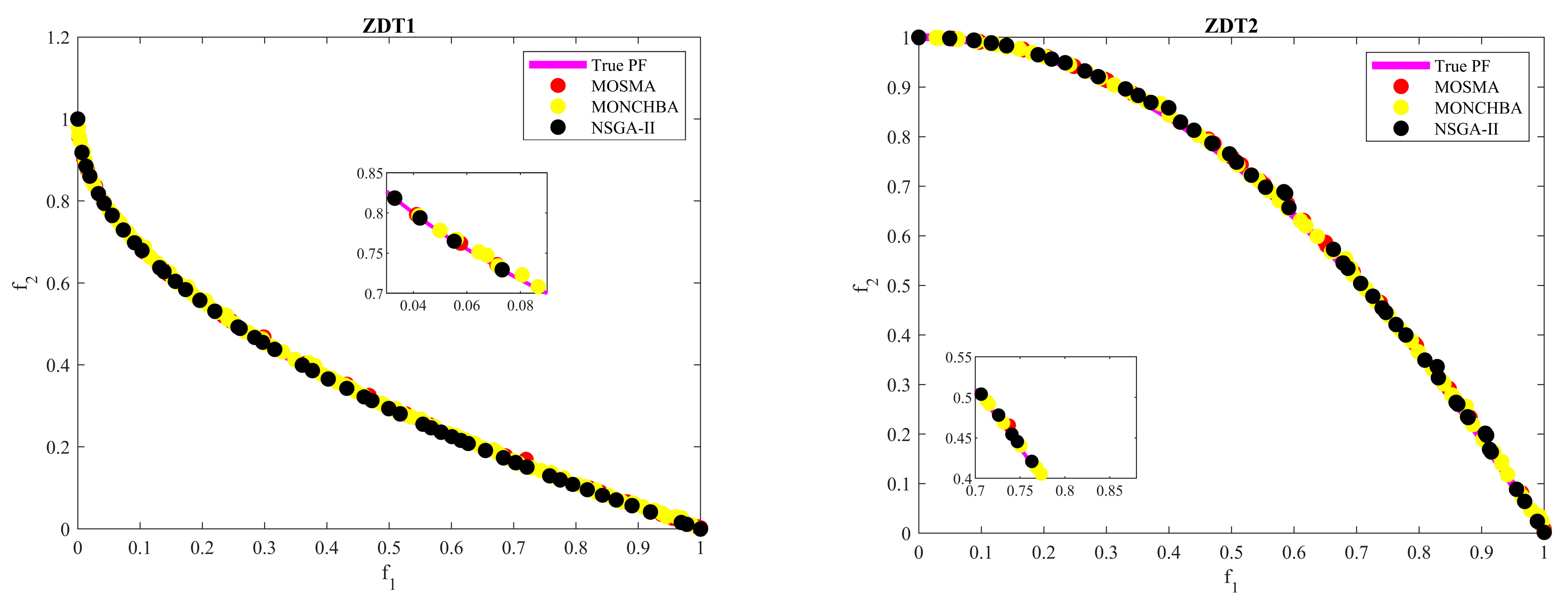
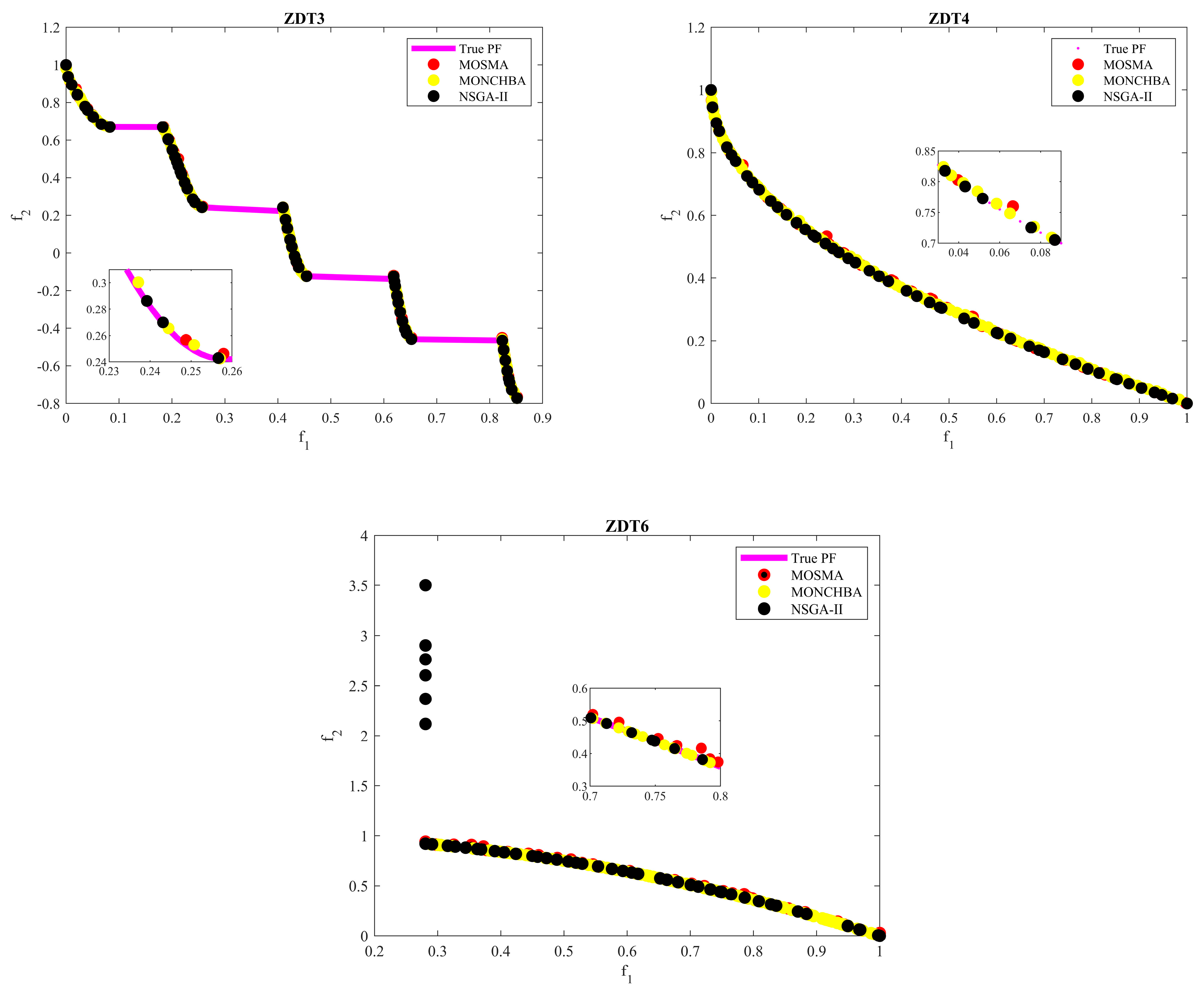
3.3. Multi-Objective NCHBA for Benchmark Problems

To address the optimization challenge in energy management for water distribution stations, the performance of MONCHBA was evaluated against two algorithms, MOSMA and NSGA-II, using five benchmark problems from the ZDT benchmark series [49]. These problems were chosen due to the highly nonlinear nature of these functions and their numerous decision variables, which pose a significant challenge for multi-objective optimization algorithms. Also, each algorithm was executed 30 times with 100 initial populations and 500 iterations to ensure the fairness of the comparison of algorithms.

Two well-known criteria, inverted generation distance (IGD) and spacing (SP), are used to evaluate the overall performance of the algorithm. The IGD is used to measure the convergence and distribution performance, and the SP is used to show the uniformity of obtained solutions by algorithms. The smallest value of the mentioned parameters shows the superiority of the algorithm compared to other algorithms [49].

$$IGD=\frac{{{\displaystyle \sum }}_{i=1}^n{d}_i}{n}$$

(27)

$$SP=\sqrt{\frac{{{\displaystyle \sum }}_{i=1}^n{\left(\overline{d}-d_i\right)}^2}{n-1}}$$

(28)

where $d_i$ is the Euclidian distance between the ith Pareto optimal solution obtained by the algorithm and the nearest true Pareto optimal solution in the reference set, $\overline{d}$ is the mean value of $d_i$, and $n$ shows the total number of achieved Pareto optimal solutions.

Table 5. The SP and IGD statistics on ZDT benchmark problems.

		IGD				SP
		Average	St.d	Best	Worst	Average	St.d	Best	Worst
ZDT1	MONCHBA	4.63 × 10−3	1.95 × 10−4	4.43 × 10−3	4.93 × 10−3	5.85 × 10−3	3.51 × 10−3	5.50 × 10−3	6.39 × 10−3
	NSGA-II	6.23 × 10−2	7.39 × 10−2	2.97 × 10−1	1.97 × 10	6.23 × 10−2	4.51 × 10−2	9.47 × 10−3	1.09 × 10−1
	MOSMA	1.21 × 10−2	7.52 × 10−2	1.48 × 10−2	3.33 × 10−2	1.21 × 10−2	4.75 × 10−2	8.96 × 10−3	1.62 × 10−2
ZDT2	MONCHBA	4.54 × 10−3	2.58 × 10−4	4.32 × 10−3	4.96 × 10−3	5.23 × 10−3	3.95 × 10−4	4.92 × 10−3	5.98 × 10−3
	NSGA-II	1.05	6.33 × 10−1	8.45 × 10−3	1.61	2.46 × 10−2	1.49 × 10−2	4.65 × 10−2	1.23 × 10−2
	MOSMA	2.98 × 10−1	2.90 × 10−1	2.46 × 10−2	7.72 × 10−1	1.21 × 10−2	4.75 × 10−2	8.96 × 10−3	1.62 × 10−2
ZDT3	MONCHBA	6.12 × 10−3	1.24 × 10−3	4.68 × 10−3	7.11 × 10−3	6.28 × 10−3	8.63 × 10−4	5.60 × 10−3	7.31 × 10−3
	NSGA-II	7.68 × 10−2	1.18 × 10−1	8.72 × 10−3	2.86 × 10−1	1.21 × 10−1	1.75 × 10−1	2.34 × 10−2	4.32 × 10−1
	MOSMA	6.05 × 10−2	1.72 × 10−2	8.76 × 10−2	4.13 × 10−2	3.35 × 10−2	4.25 × 10−2	1.91 × 10−2	4.65 × 10−2
ZDT4	MONCHBA	4.80 × 10−3	2.70 × 10−4	4.47 × 10−3	5.22 × 10−3	5.87 × 10−3	5.49 × 10−3	5.18 × 10−3	6.36 × 10−3
	NSGA-II	3.71	2.33	7.77 × 10−1	6.45	6.50 × 10−1	3.73 × 10−1	1.90 × 10−1	1.08
	MOSMA	4.75 × 10	2.43 × 10	1.94 × 10	7.45 × 10	2.64	1.12 × 10−2	1.23 × 10−1	5.15
ZDT6	MONCHBA	3.33 × 10−3	4.37 × 10−4	2.69 × 10−3	3.82 × 10−3	5.05 × 10−3	4.34 × 10−4	4.60 × 10−3	5.73 × 10−3
	NSGA-II	5.69 × 10−2	2.02 × 10−2	3.55 × 10−2	8.47 × 10−2	5.99 × 10−2	4.75 × 10−2	1.34 × 10−1	2.28 × 10−2
	MOSMA	5.16 × 10−1	1.14	3.89 × 10−3	2.55	8.72 × 10−2	3.33 × 10−1	1.86 × 10−2	2.22 × 10−1

displays the amounts of IGD and SP statistical indices for algorithms in solving ZDT functions. As it is clear, MONCHBA has solved ZDT problems well. Based on IGD, a criterion of convergence of algorithms, it is clear that MONCHBA had better convergence compared to the other two algorithms for solving ZDT functions. Also, considering that the SP criterion shows the uniformity of the solutions obtained, MONCHBA can produce solutions with a suitable and uniform distribution.

Figure 6 represents the optimal Pareto fronts obtained by three algorithms, MONCHBA, MOSMA, and NSGA-II, for problems of ZDT₁ to ZDT₄ and ZDT₆. The optimal solution set of all three algorithms is uniformly converged to the actual Pareto front. By enlarging a part of the Pareto front, the uniformity of the solutions of the MONCHBA algorithm was much higher than the other two algorithms. At the same time, MOSMA has not been able to adapt effectively to the actual Pareto. The convergence of three algorithms for the ZDT₂ problem in Figure 6 shows the reasonable accuracy of MONCHBA compared to the other two algorithms. Hence, the solutions found by NSGA-II were far better than those found by MOSMA. However, the number of solutions obtained is less than the other two algorithms. This figure shows that the convergence of the proposed algorithm in solving the ZDT₃ function is also acceptable. The set of solutions provided by it is uniformly converged to the true Pareto front in the interaction diagram of the ZDT₄ and ZDT₆ examples presented in Figure 6, and it is the same as the algorithm MONCGWO has good accuracy and convergence. However, the noteworthy point is the poor performance of the MOSMA algorithm compared to the other two algorithms, which failed to converge accurately with the true solution. The optimal solutions were placed far from the true Pareto in almost all examples, meaning the weakness of this algorithm in escaping local optima and premature convergence.

Examining the results of modeling the benchmark functions using the proposed multi-objective algorithm reveals that the performance of the initial version of the HBA algorithm has been improved through the utilization of the chaotic approach. This improvement is evident in the algorithm’s ability to produce accurate answers in accordance with the real answers when solving the benchmark problems. This success can be attributed to the proper interaction between the search and exploration phases.

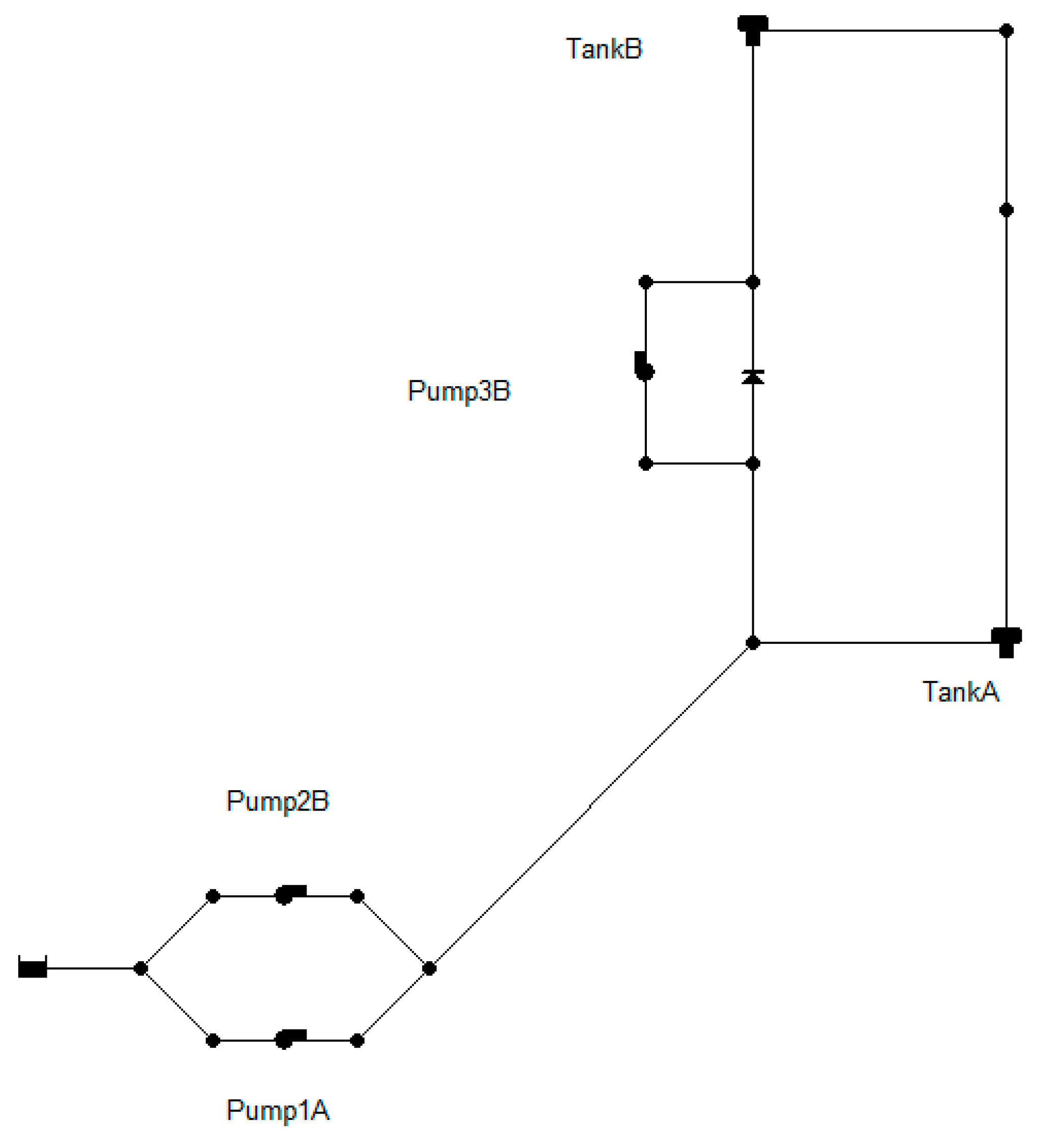
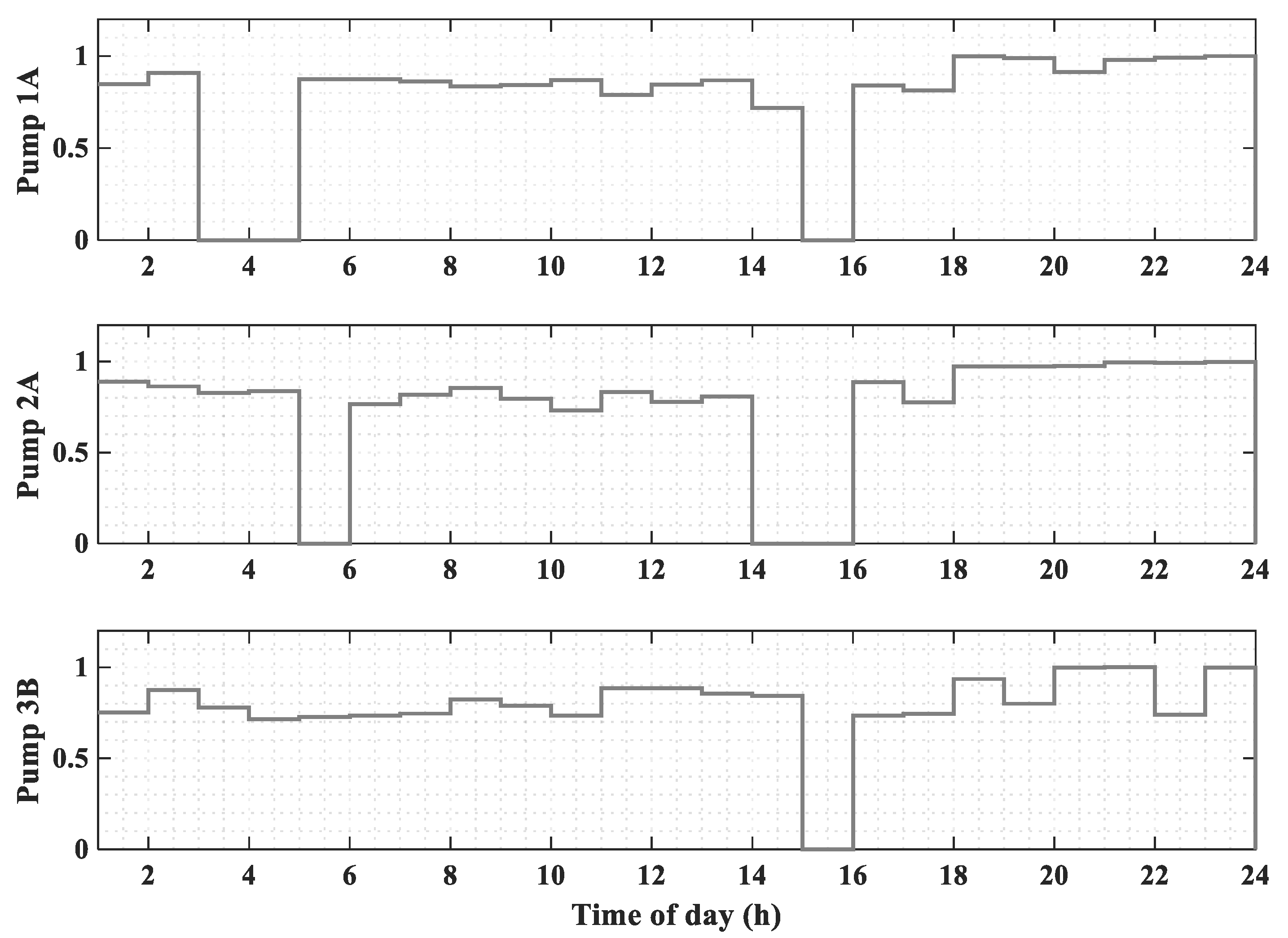
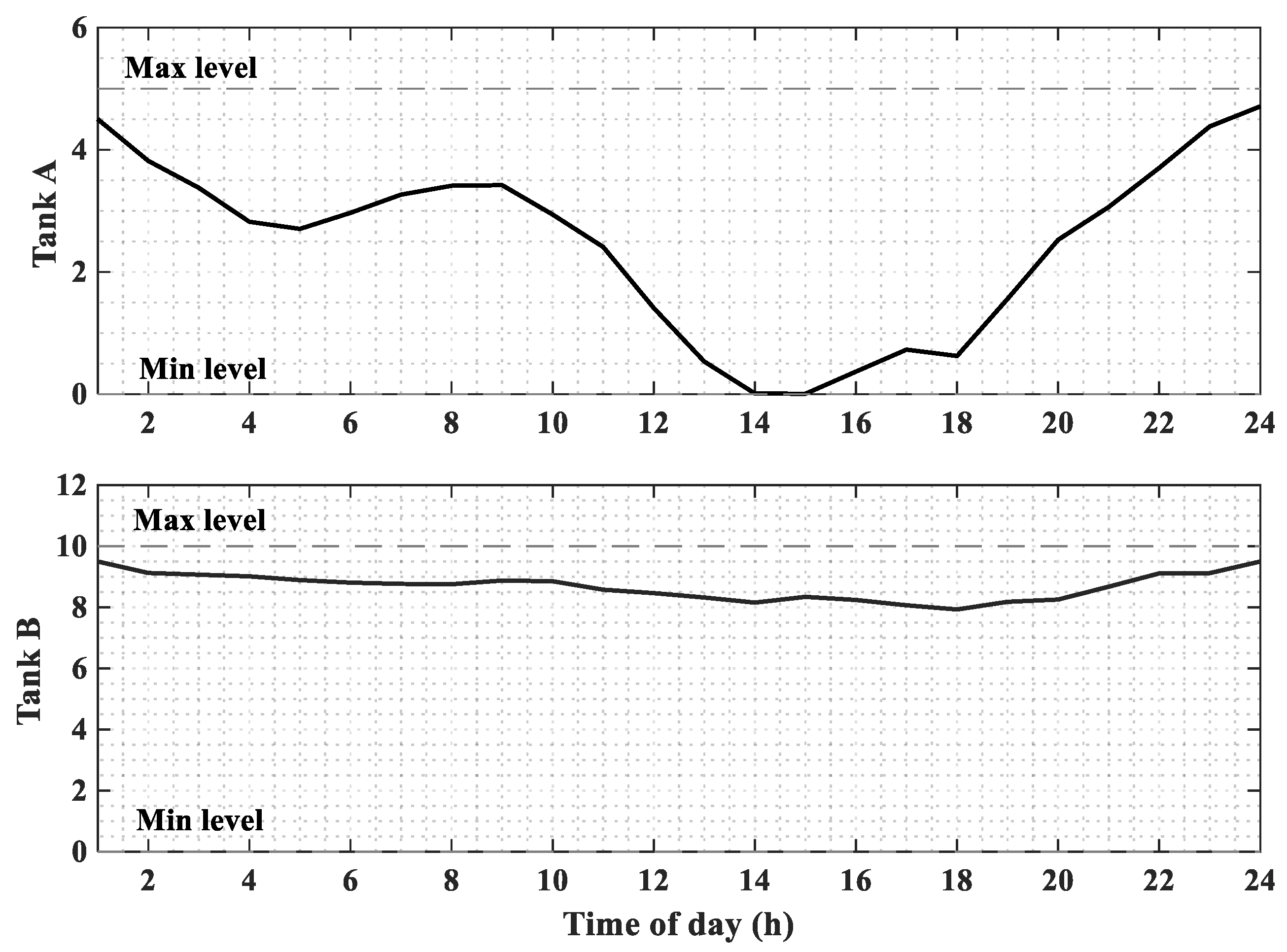
3.4. Multi-Objective NCHBA for Energy Optimization

The problem of exploiting WDSs was examined as a multi-objective optimization problem in this section. The first, second, and third objectives were to minimize the cost of energy consumption, the network pressure level, and the quality risk of the network, respectively. For this purpose, the objective functions and constraints introduced in Section 2.2 were used in the optimization process. The WDS used in this section is the C-Town network (Figure 7), a large-scale WDS with 399 consumption nodes, 443 pipes, seven storage tanks, 11 pumps, five valves, and the main water supply reservoir. The C-Town network was divided into five district metered areas (DMAs) for easy management and operation, each with a different hourly consumption pattern. The C-Town network distributed water from the main reservoir to the two storage tanks, T1 and T2, by pumping station S1. Notably, the transfer flow to tank T2 was controlled by valve V₂ based on the water level in the tank. Pumping stations S2 and S3 transferred water from the T2 tank to the tanks located at a higher altitude. Pumping stations S4 and S5 were responsible for transferring water from tank T1 to tanks T5, T6, and T7. Figure 7 shows the schematic of this network.

The operation details of C-Town are available at: https://www.exeter.ac.uk/media/universityofexeter/emps/research/cws/downloads/d-town.inpl, accessed on 13 March 2024 (Expansion|Engineering|University of Exeter).

Two scenarios were proposed and evaluated according to the study’s objectives to determine an operation plan for the WSD pumps. Firstly, the pumps in the network were considered variable-speed pumps, and the multi-purpose operation of the pumping stations was discussed. Then, the modeling was conducted by considering the constant-speed pump in the stations. Notably, the number of decision variables in the simulation–optimization model developed using the MONCHBA multi-objective algorithm and the EPANET simulator was equal to 264. For the first scenario, it was required to obtain the optimal speed of the pumps. In addition to complying with the constraints of the problem, including the permissible range of changes in the water level of the storage tanks and the minimum operating pressure, it provided a satisfying interaction between the goals of minimizing pumping energy costs, the network pressure level, and reducing water age-based risk. The first modeling results were presented as a three-dimensional Pareto diagram in Figure 8. As it is known, the model has provided various solutions with different kinds of quality-based risk levels, pressure levels, and the cost of energy consumed in the network.

A favorable distribution of the points found on the Pareto front indicates the precision of MONCHBA. Accordingly, the lowest and highest value of network quality risk ranged between 14.5% and 19%. With the increase in the second objective function, the value of quality risks declined, and vice versa, which can be due to the increase in leakage, consumption, and, as a result, the decline of water age in the network. It can also be said that the water quality risk also decreased with the increase in energy costs and increased network consumption. Based on this, the conflict between quality risk, pumping costs, and network pressure level was apparent. According to the graph of the interaction between two energy and pressure functions, with the increase in pumping costs, the pressure level in the network increased, which was an obvious issue.

In multi-objective optimization problems, none of the solutions on the Pareto front is preferable to the other, and the employer can choose any of the solutions based on the available budget. The fuzzy decision-making method was used to comment more on the impact of variable-speed pumps on water quality and network pressure. An optimal answer establishes a suitable interaction between all three objectives. The fuzzy decision-making method is implemented as follows [50]:

$${\mu }_i^j=\{\begin{array}{cc}\hfill 1, \hfill & if f_i^j<f_{min}^j\\ \hfill \frac{f_{max}^j-f_i^j}{f_{max}^j-f_{min}^j,}\hfill & \hspace{1em}if{f}_{min}^j\le f_i^j\le f_{max}^j \\ \hfill 0, \hfill & if f_i^j>f_{max}^j\end{array}$$

(29)

After calculating ${\mu }_i^j$ for each point obtained on the Pareto front, the fuzzy membership function (${\mu }_i$) is computed using Equation (30). The value of ${\mu }_i$ ranges between 0 and 1 and is estimated as a vector for each series of answers (i.e., f₁, f₂, and f₃). The answer series with the highest ${\mu }_i$ value is chosen as the final answer, indicating a consensus among all objectives.

$${\mu }_i\left(Normalized\right)=\frac{{{\displaystyle \sum }}_{j=1}^{N_{obj}}{\mu }_{ij}}{{{\displaystyle \sum }}_{i=1}^M{{\displaystyle \sum }}_{j=1}^{N_{obj}}{\mu }_{ij}}$$

(30)

where M is the number of solutions, $N_{obj}$ indicates the number of objective functions, and $f_{min}^j$ and $f_{max}^j$ are the minimum and maximum values of the objective function, respectively. ${\mu }_i$ is the membership function.

Based on the solution presented in the above approach, indicated by a different color in the Pareto front, the values of the objective functions of energy, pressure level, and quality risk of the network were obtained as 1189.14$, 415,958 m, and 16%, respectively.

In the second model, by using the transfer function approach, the MONCHBA search space was converted into a binary space, and the simulation–optimization model was implemented assuming constant-speed pumps. The results of running the developed model with binary space on the C-Town water distribution network are presented in Figure 9, similar to the previous scenario.

The Pareto model (1) has a more appropriate distribution than the Pareto model (2), which can be caused by the complexity of the problem space in binary mode and the high number of decision variables. According to the researcher’s experience, achieving better results by using variable-speed pumps was not unexpected. The continuous and slow rotation speed change in variable-speed pumps compared to the sudden turning off/on of fixed-speed pumps makes it difficult to achieve proper interaction in the large-scale problem.

According to the Pareto front, the lowest and highest values of quality-based risk in the network were 17.5% and 22.5%, respectively, meaning an increase compared to scenario number (1). The energy consumption costs in the ranges of USD 1180–1280 and USD 1100–1500 for the fixed and variable-speed pumps, respectively, were considerable. The flexibility of the network resulted from using variable-speed pumps, which give the employer multiple options. To achieve a better comparison, one of the responses on the Pareto front in Figure 8 and Figure 9 was selected and analyzed using the fuzzy decision-making method.

The values of the objective functions of the problem in the case of fixed-speed pumps for the optimal response obtained for the first, second, and third objective functions were 1215.24$ and 415,131.2 m, 19%, respectively. Hence, using variable-speed pumps instead of fixed-speed pumps is also effective and highly efficient in multi-purpose operating conditions. To better compare responses, pressure level, and network quality in 24:00 h, 10:00, and 18:00, a day of operation is presented in Figure 10, Figure 11 and Figure 12.

Accordingly, by using a multi-criteria optimization approach in the operation of pumping stations and reducing energy costs, a WDS with high reliability from a qualitative and hydraulic point of view can be achieved. In general, the use of variable-speed pumps compared to fixed-speed pumps reduces the quality risk of the network and increases its reliability during operation.

It should be noted that the pressure level in the network in the presence of variable-speed pumps is higher than fixed-speed pumps in most cases, which can increase the rate of pipe failure and leakage. Therefore, it is possible to prevent the occurrence of higher pressures in different water networks based on the final tolerable pressure of the pipes by defining the maximum pressure range. In case study number (2), the maximum pressure requirement is not taken into account, and only compliance with the minimum desired pressure requirement of 20 m is considered. The schedule of C-Town water distribution network pumps is presented in Figure 13 for two scenarios. As can be seen in this figure, variable-speed pumps operate at an appropriate speed ratio for most of the day. For this reason, reducing the number of additional switching operations resulted in a full supply of node pressure and reduced operating costs.

As can be seen, using an efficient optimizer to find the optimal scheduling program of pumping stations can significantly reduce the cost of energy consumption in WDSs. The cost reductions due to using variable-speed pumps instead of single-speed pumps in the first and second case studies are caused by the proper scheduling obtained by NCHBA, which resulted in less use of the power electricity.

4. Discussion

The results presented in this study demonstrated that the proposed NCHBA outperformed other search methods, including AO, HGA, SMA, GA, EA, ABC, FA, BDA, ACO, Run, NSGA-II, and MOSMA, as well as the original version of HBA, in two phases: (1) mathematical benchmark functions and* (2) pump scheduling program optimization. The key factor behind these improvements lies in the modification of the HBA operators, notably the inclusion of a chaotic map and a nonlinear mechanism, along with the addition of a crossover operator to the multi-objective version of the algorithm. These additional mechanisms effectively enhanced the algorithm’s ability to perform both global and local searches. The crossover operator plays a vital role in diversifying the population, thereby aiding the proposed algorithm in discovering more promising solutions. The implementation of the NCHBA further improves the search for the optimal solutions, enabling the identification of a greater number of favorable solutions. The results demonstrate the efficiency of the proposed algorithm in effectively solving intricate mathematical test functions. Furthermore, the outcomes of both single and multi-objective pump scheduling programs validate the remarkable capability of NCHBA in optimizing pump speeds, thereby effectively reducing the water conveyance footprint.

It is important to acknowledge and address the potential limitations of this study. Despite the fact that incorporating new mechanisms into any optimization algorithm enhances both the convergence speed and accuracy, this improvement comes at the expense of increased computational costs, particularly for complex water distribution systems (WDSs) with numerous variables, such as pressure-reducing valves and pump statuses. To overcome this drawback, the implementation of parallel computing technology can be effective. Furthermore, it is important to note that despite the excellent performance of the proposed algorithm, it is essential to acknowledge the limitations outlined in the “no free lunch (NFL)” theorem. This theorem emphasizes that there is no universal optimizer capable of efficiently solving all complex problems related to WDSs.

5. Conclusions

Sustainable operation and management of water distribution systems (WDSs) is a complex, multi-faceted, and challenging optimization problem characterized by numerous decision variables, complicated constraints, and multiple objective functions. This study focuses on addressing the optimization problem of pump scheduling in WDSs. To tackle this challenge, a novel and enhanced optimization algorithm, namely NCHBA, was introduced. The NCHBA incorporates a chaotic map and a nonlinear mechanism to further improve its performance. The proposed algorithm was coupled with the EPANET model to estimate the response of the WDSs according to the optimal schedule. The proposed model was utilized to optimize the energy consumption in variable-speed pumps in a benchmark network. The performance of the proposed NCHBA is compared with five meta-heuristic algorithms (i.e., AO, HGA, RUN, SMA, and HBA). The results confirm that the proposed NCHB outperforms the original HBA for the single objective pump scheduling problem and also reduces energy consumption more than any other algorithm. The implementation of the proposed NCHB resulted in significant energy cost savings, reaching up to 27% for the case study pumping station. Hence, the proposed approach can facilitate a significant reduction in a WDS footprint.

The proposed algorithm was converted into a multi-objective algorithm using the crossover approach, and it was utilized to reduce the water conveyance footprint in WDSs. ZDT series test functions were used to evaluate the performance of the algorithm. The efficiency of the proposed method for a large-scale water network was successfully investigated by considering the minimization of energy consumption, water quality risk, and pressure deficit as objective functions. The optimization-simulation model developed based on the new algorithm was implemented to assess two scenarios with variable-speed and fixed-speed network pumps. The results showed that the variable-speed pumps have a high potential to reduce water conveyance footprint in WDSs. The appropriateness and robustness of the proposed NCHBS approach should be further validated for different objectives of WDS management. For example, future studies can assess the performance of NCHBA to optimize the location of pumps as turbines or PRVs in WDSs. Further research is needed to investigate the accuracy and reliability of EPANET for estimating the energy consumption of variable-speed pumps.

References

1. Ang, W.K.; Jowitt, P.W. Some new insights on informational entropy for water distribution networks. Eng. Optim. 2005, 37, 277–289. [Google Scholar] [CrossRef]
2. Latifi, M.; Farahi Moghadam, K.; Naeeni, S.T. Pressure and energy management in water distribution networks through optimal use of Pump-As-Turbines along with pressure-reducing valves. J. Water Resour. Plan. Manag. 2021, 147, 04021039. [Google Scholar] [CrossRef]
3. Gheisi, A.; Naser, G. Multistate reliability of water-distribution systems: Comparison of surrogate measures. J. Water Resour. Plan. Manag. 2015, 141, 04015018. [Google Scholar] [CrossRef]
4. Van Zyl, J.E.; Savic, D.A.; Walters, G.A. Operational optimization of water distribution systems using a hybrid genetic algorithm. J. Water Resour. Plan. Manag. 2004, 130, 160–170. [Google Scholar] [CrossRef]
5. Jowitt, P.W.; Germanopoulos, G. Optimal pump scheduling in water-supply networks. J. Water Resour. Plan. Manag. 1992, 118, 406–422. [Google Scholar] [CrossRef]
6. Ormsbee, L.E.; Walski, T.M.; Chase, D.V.; Sharp, W.W. Methodology for improving pump operation efficiency. J. Water Resour. Plan. Manag. 1989, 115, 148–164. [Google Scholar] [CrossRef]
7. Chase, D.V.; Ormsbee, L.E. Computer-Generated Pumping Schedules for Satisfying Operational Objectives. J. Am. Water Work. Assoc. 1993, 85, 54–61. [Google Scholar] [CrossRef]
8. Lansey, K.E.; Awumah, K. Optimal pump operations considering pump switches. J. Water Resour. Plan. Manag. 1994, 120, 17–35. [Google Scholar] [CrossRef]
9. Nitivattananon, V.; Sadowski, E.C.; Quimpo, R.G. Optimization of water supply system operation. J. Water Resour. Plan. Manag. 1996, 122, 374–384. [Google Scholar] [CrossRef]
10. Pasha, M.F.; Lansey, K. Strategies to develop warm solutions for real-time pump scheduling for water distribution systems. Water Resour. Manag. 2014, 28, 3975–3987. [Google Scholar] [CrossRef]
11. Afshar, M.H.; Rajabpour, R. Application of local and global particle swarm optimization algorithms to optimal design and operation of irrigation pumping systems. Irrig. Drain. J. Int. Comm. Irrig. Drain. 2009, 58, 321–331. [Google Scholar] [CrossRef]
12. Ebrahimi, S.; Riasi, A.; Kandi, A. Selection optimization of variable speed pump as turbine (PAT) for energy recovery and pressure management. Energy Convers. Manag. 2021, 227, 113586. [Google Scholar] [CrossRef]
13. Soltani, M.; Nabat, M.H.; Razmi, A.R.; Dusseault, M.B.; Nathwani, J. A comparative study between ORC and Kalina based waste heat recovery cycles applied to a green compressed air energy storage (CAES) system. Energy Convers. Manag. 2020, 222, 113203. [Google Scholar] [CrossRef]
14. Li, M.; Zhao, L.; Zhang, C.; Liu, Y.; Fu, Q. Optimization of agricultural resources in water-energy-food nexus in complex environment: A perspective on multienergy coordination. Energy Convers. Manag. 2022, 258, 115537. [Google Scholar] [CrossRef]
15. Barbarelli, S.; Amelio, M.; Florio, G. Experimental activity at test rig validating correlations to select pumps running as turbines in microhydro plants. Energy Convers. Manag. 2017, 149, 781–797. [Google Scholar] [CrossRef]
16. Lydon, T.; Coughlan, P.; McNabola, A. Pressure management and energy recovery in water distribution networks: Development of design and selection methodologies using three pump-as-turbine case studies. Renew. Energy 2017, 114, 1038–1050. [Google Scholar] [CrossRef]
17. Moazeni, F.; Khazaei, J. Optimal operation of water-energy microgrids; a mixed integer linear programming formulation. J. Clean. Prod. 2020, 275, 122776. [Google Scholar] [CrossRef]
18. Moazeni, F.; Khazaei, J.; Mendes, J.P.P. Maximizing energy efficiency of islanded micro water-energy nexus using co-optimization of water demand and energy consumption. Appl. Energy 2020, 266, 114863. [Google Scholar] [CrossRef]
19. Bagirov, A.M.; Barton, A.F.; Mala-Jetmarova, H.; Al Nuaimat, A.; Ahmed, S.T.; Sultanova, N.; Yearwood, J. An algorithm for minimization of pumping costs in water distribution systems using a novel approach to pump scheduling. Math. Comput. Model. 2013, 57, 873–886. [Google Scholar] [CrossRef]
20. López-Ibáñez, M. Operational Optimisation of Water Distribution Networks. Ph.D. Thesis, Edinburgh Napier University, Edinburgh, UK, 2009. [Google Scholar]
21. Jafari-Asl, J.; Azizyan, G.; Monfared, S.A.H.; Rashki, M.; Andrade-Campos, A.G. An enhanced binary dragonfly algorithm based on a V-shaped transfer function for optimization of pump scheduling program in water supply systems (case study of Iran). Eng. Fail. Anal. 2021, 123, 105323. [Google Scholar] [CrossRef]
22. Farmani, R.; Walters, G.A.; Savic, D.A. Trade-off between total cost and reliability for Anytown water distribution network. J. Water Resour. Plan. Manag. 2005, 131, 161–171. [Google Scholar] [CrossRef]
23. Abiodun, F.T.; Ismail, F.S. Pump scheduling optimization model for water supply system using AWGA. In Proceedings of the 2013 IEEE Symposium on Computers & Informatics (ISCI), Langkawi, Malaysia, 7–9 April 2013; pp. 12–17. [Google Scholar]
24. Kurek, W.; Ostfeld, A. Multi-objective optimization of water quality, pumps operation, and storage sizing of water distribution systems. J. Environ. Manag. 2013, 115, 189–197. [Google Scholar] [CrossRef]
25. Makaremi, Y.; Haghighi, A.; Ghafouri, H.R. Optimization of pump scheduling program in water supply systems using a self-adaptive NSGA-II; a review of theory to real application. Water Resour. Manag. 2017, 31, 1283–1304. [Google Scholar] [CrossRef]
26. Price, E.; Ostfeld, A. Optimal pump scheduling in water distribution systems using graph theory under hydraulic and chlorine constraints. J. Water Resour. Plan. Manag. 2016, 142, 04016037. [Google Scholar] [CrossRef]
27. Mala-Jetmarova, H.; Barton, A.; Bagirov, A. Exploration of the trade-offs between water quality and pumping costs in optimal operation of regional multiquality water distribution systems. J. Water Resour. Plan. Manag. 2015, 141, 04014077. [Google Scholar] [CrossRef]
28. Castro-Gama, M.; Pan, Q.; Lanfranchi, E.A.; Jonoski, A.; Solomatine, D.P. Pump scheduling for a large water distribution network. Milan, Italy. Procedia Eng. 2017, 186, 436–443. [Google Scholar] [CrossRef]
29. Yan, P.; Zhang, Z.; Lei, X.; Hou, Q.; Wang, H. A multi-objective optimal control model of cascade pumping stations considering both cost and safety. J. Clean. Prod. 2022, 345, 131171. [Google Scholar] [CrossRef]
30. Guo, S.; Song, G.; Li, M.; Zhao, X.; He, Y.; Kurban, A.; Ji, W.; Wang, J. Multi-objective bi-level quantity regulation scheduling method for electric-thermal integrated energy system considering thermal and hydraulic transient characteristics. Energy Convers. Manag. 2022, 253, 115147. [Google Scholar] [CrossRef]
31. Jafari-Asl, J.; Seghier, M.E.A.B.; Ohadi, S.; van Gelder, P. Efficient method using Whale Optimization Algorithm for reliability-based design optimization of labyrinth spillway. Appl. Soft Comput. 2021, 101, 107036. [Google Scholar] [CrossRef]
32. Rad, M.J.G.; Ohadi, S.; Jafari-Asl, J.; Vatani, A.; Ahmadabadi, S.A.; Correia, J.A. GNDO-SVR: An efficient surrogate modeling approach for reliability-based design optimization of concrete dams. Structures 2022, 35, 722–733. [Google Scholar] [CrossRef]
33. Rahmanshahi, M.; Jafari-Asl, J.; Fathi-Moghadam, M.; Ohadi, S.; Mirjalili, S. Metaheuristic learning algorithms for accurate prediction of hydraulic performance of porous embankment weirs. Appl. Soft Comput. 2024, 151, 111150. [Google Scholar] [CrossRef]
34. Hashim, F.A.; Houssein, E.H.; Hussain, K.; Mabrouk, M.S.; Al-Atabany, W. Honey Badger Algorithm: New metaheuristic algorithm for solving optimization problems. Math. Comput. Simul. 2022, 192, 84–110. [Google Scholar] [CrossRef]
35. Rossman, L.A. EPANET 2: User’s Manual; U.S. Environmental Protection Agency: Cincinnati, OH, USA, 2000. [Google Scholar]
36. Coelho, B. Energy Efficiency of Water Supply Systems Using Optimisation Techniques and Micro-Hydroturbines. Ph.D. Thesis, Universidade de Aveiro, Aveiro, Portugal, 2016. [Google Scholar]
37. Shokoohi, M.; Tabesh, M.; Nazif, S.; Dini, M. Water quality based multi-objective optimal design of water distribution systems. Water Resour. Manag. 2017, 31, 93–108. [Google Scholar] [CrossRef]
38. Wagner, J.M.; Shamir, U.; Marks, D.H. Water distribution reliability: Simulation methods. J. Water Resour. Plan. Manag. 1988, 114, 276–294. [Google Scholar] [CrossRef]
39. Dehkordi, A.A.; Sadiq, A.S.; Mirjalili, S.; Ghafoor, K.Z. Nonlinear-based chaotic harris hawks optimizer: Algorithm and internet of vehicles application. Appl. Soft Comput. 2021, 109, 107574. [Google Scholar] [CrossRef]
40. Mirjalili, S.; Gandomi, A.H.; Mirjalili, S.Z.; Saremi, S.; Faris, H.; Mirjalili, S.M. Salp Swarm Algorithm: A bio-inspired optimizer for engineering design problems. Adv. Eng. Softw. 2017, 114, 163–191. [Google Scholar] [CrossRef]
41. Houssein, E.H.; Çelik, E.; Mahdy, M.A.; Ghoniem, R.M. Self-adaptive Equilibrium Optimizer for solving global, combinatorial, engineering, and Multi-Objective problems. Expert Syst. Appl. 2022, 195, 116552. [Google Scholar] [CrossRef]
42. Li, S.; Chen, H.; Wang, M.; Heidari, A.A.; Mirjalili, S. Slime mould algorithm: A new method for stochastic optimization. Future Gener. Comput. Syst. 2020, 111, 300–323. [Google Scholar] [CrossRef]
43. Abualigah, L.; Yousri, D.; Abd Elaziz, M.; Ewees, A.A.; Al-Qaness, M.A.; Gandomi, A.H. Aquila optimizer: A novel meta-heuristic optimization algorithm. Comput. Ind. Eng. 2021, 157, 107250. [Google Scholar] [CrossRef]
44. Yang, Y.; Chen, H.; Heidari, A.A.; Gandomi, A.H. Hunger games search: Visions, conception, implementation, deep analysis, perspectives, and towards performance shifts. Expert Syst. Appl. 2021, 177, 114864. [Google Scholar] [CrossRef]
45. Ahmadianfar, I.; Heidari, A.A.; Gandomi, A.H.; Chu, X.; Chen, H. RUN beyond the metaphor: An efficient optimization algorithm based on Runge Kutta method. Expert Syst. Appl. 2021, 181, 115079. [Google Scholar] [CrossRef]
46. Bagirov, A.; Ahmed, S.; Barton, A.; Mala-Jetmarova, H.; Al Nuaimat, A.; Sultanova, N. Comparison of metaheuristic algorithms for pump operation optimization. In Proceedings of the 14th Water Distribution Systems Analysis Conference 2012, Adelaide, SA, Australia, 24–27 September 2012; pp. 886–896. [Google Scholar]
47. López-Ibáñez, M.; Prasad, T.D.; Paechter, B. Representations and evolutionary operators for the scheduling of pump operations in water distribution networks. Evol. Comput. 2011, 19, 429–467. [Google Scholar] [CrossRef]
48. Hashemi, S.S.; Tabesh, M.; Ataeekia, B. Ant-colony optimization of pumping schedule to minimize the energy cost using variable-speed pumps in water distribution networks. Urban Water J. 2014, 11, 335–347. [Google Scholar] [CrossRef]
49. Li, L.L.; Ren, X.Y.; Tseng, M.L.; Wu, D.S.; Lim, M.K. Performance evaluation of solar hybrid combined cooling, heating and power systems: A multi-objective arithmetic optimization algorithm. Energy Convers. Manag. 2022, 258, 115541. [Google Scholar] [CrossRef]
50. Mellal, M.A.; Zio, E.; Pecht, M. Multi-objective reliability and cost optimization of fuel cell vehicle system with fuzzy feasibility. Inf. Sci. 2023, 640, 119112. [Google Scholar] [CrossRef]
Figure 1. The proposed simulation–optimization framework.
Water 16 00874 g001
Figure 2. Schematic of case study I.
Water 16 00874 g002
Figure 3. Convergence curve of NCHBA and other algorithms for case study I.
Water 16 00874 g003
Figure 4. Pumps operation program for case study I.
Water 16 00874 g004
Figure 5. Tanks operation level for case study I.
Water 16 00874 g005
Figure 6. Pareto fronts of three algorithms on ZDT functions.
Water 16 00874 g006aWater 16 00874 g006b
Figure 7. Schematic of C-Town network.
Water 16 00874 g007
Figure 8. The optimal Pareto front obtained using MONCHBO for Scenario 1.
Water 16 00874 g008
Figure 9. The optimal Pareto front obtained using MONCHBO for Scenario 2.
Water 16 00874 g009
Figure 10. Situation of C-Town WDS in terms of pressure and water age at 24:00: (a) Scenario 2; (b) Scenario 1.
Water 16 00874 g010
Figure 11. Situation of C-Town WDS in terms of pressure and water age at 10:00: (a) Scenario 2; (b) Scenario 1.
Water 16 00874 g011
Figure 12. Situation of C-Town WDS in terms of pressure and water age at 18:00: (a) Scenario 2; (b) Scenario 1.
Water 16 00874 g012
Figure 13. The pump scheduling program of C-Town for scenarios 1 and 2.
Water 16 00874 g013