Article

Swash-Zone Formula Evaluation of Morphological Variation in Haeundae Beach, Korea

1
East Sea Environment Research Center, Korea Institute of Ocean Science and Technology, Uljin 36315, Republic of Korea
2
Sekwang Engineering Consultant Company Limited, Seoul 08381, Republic of Korea
3
Maritime ICT & R&D Center, Korea Institute of Ocean Science and Technology, Busan 49111, Republic of Korea
*
Author to whom correspondence should be addressed.
Water 2024, 16(6), 836; https://doi.org/10.3390/w16060836
Submission received: 19 January 2024 / Revised: 10 March 2024 / Accepted: 12 March 2024 / Published: 14 March 2024
(This article belongs to the Special Issue Coastal Sediments: Processes, Transport, Modeling and Hydrodynamics)

Abstract

:
In this study, a swash-zone model, using Larson and Wamsley formula (LW07), was combined into the Telemac-2D model system to examine the performance of modeling swash-zone processes through comparisons with field observation data. The experimental site was the Haeundae Beach in South Korea where Typhoon Phanfone occurred in October 2014, and bathymetric surveys were performed before and after the typhoon. Hydrodynamic data were also measured to validate the modeled data. The performance of LW07 was tested by running the model in two modes, with and without LW07. First, the model was run to simulate the shoreline response to an imaginary coastal breakwater. The result showed a clear discrepancy between the two modes as the sediments were considerably cumulated behind the breakwater in the case with the swash-zone formula (LW07) in the wide range along the shoreline behind the breakwater, indicating that the sediments more actively and rapidly responded to the shadowing by the breakwater with LW07. The model was also run for a realistic case from August to October 2014, which included the typhoon’s period during 2–6 October. The results showed that the morphological changes at both ends of the beach in the swash zone were simulated with higher accuracy with LW07, supporting the effectiveness of LW07 in simulating the short-term morphological changes induced by the typhoon attack. In particular, the successful simulation of the sand accumulation at the end sides of the beach’s swash zone indicates that LW07 was effective in estimating not only the cross-shore transport but also longshore transport, which was likely due to the characteristics of LW07 that calculated sand transport in both directions. The enhanced modeling performance with LW07 was likely due to the adjustment of the sediment transport rate to the instantaneous changes in the local beach slope, which could successfully control the erosion/accretion process in the swash zone more realistically.

1. Introduction

Beach erosion is an important issue in many countries, as it causes economic damage to the local community when the value of beaches is reduced by the loss of sand. To protect beach sand from erosional damages, it is crucial to accurately predict the erosional or depositional processes on the beach face, and numerical models have been commonly used for such predictions. One of the available numerical tools is the line models based on the single-line theory [1]. The benefit of the use of line models is clear as they can calculate long-term shoreline changes [2,3]. However, the accuracy of line models is relatively low because they only consider the longshore sediment transport gradient in estimating the spatial and temporal variation in the shorelines, so that the contributions made by the cross-shore transport and the nearshore flow circulations are not included.
To overcome the limitations of these line models, area models that calculate three-dimensional flow fields are available for the prediction of morphological changes in nearshore regions [4]. The advantages of three-dimensional modeling for beach processes include that these models can consider the effect of the three-dimensional structure of wind-induced flows and surface wave breaking. Due to the enhancement of computational capacity, the time scale that can be simulated in three-dimensional models is increasing. However, the high modeling cost still restricts their applications from extending to experiments spanning longer than a few months. In the middle course between the two extreme approaches, the two-dimensional ‘2DH’ models are more widely applied as they effectively calculate the sediment transport and the consequent bottom topography change based on the depth-integrated and phase-averaged flow and wave fields [5,6,7,8,9,10,11,12,13,14,15].
Although 2DH models are useful in the prediction of morphological changes, their shortcomings are also evident as they are not able to consider the effect of undertows in the surf zone where the seabed elevation actively changes. In addition, since 2DH models treat the shoreline as a solid boundary, they cannot directly calculate variation in the shorelines over time and thus are not able to provide quantitatively meaningful information on the shoreline evolution. Another weakness of 2DH models lies in controlling the swash zone. In the swash zone, wave energy is actively transferred to kinetic energy during the uprush and backwash of the waves, which produces strong sediment motions within the waves. Therefore, the hydrodynamic process in this boundary area between the land and the sea plays a significant role in calculating the nearshore sediment transport rates and the consequent morphological changes. However, since observations in the swash zone are extremely difficult due to the waves splashing and the rapid change in the shallow water level, a correct understanding of the physical process in the swash zone is still limited and thus can hardly be counted in most of the available 2HD models thus far.
Recently, Chen et al. [16] reviewed swash-zone sediment processes by comparing existing practical transport models, describing the detailed cross-shore processes such as sand motions during uprush and backwash and wave–swash interactions. Their review also compared existing practical models for swash sand transport that depended on parameterizations of small-scale processes. For example, the models were divided into three categories—empirical sand transport formulae, sand transport distribution methods, and the equilibrium concept model. However, these existing practical swash-zone sand transport models had their limitations. In order to develop and/or improve a practical model applicable for a wide range of conditions, an extensive validation of the practical model over different time scales and different beach states was needed [16].
In this study, we applied Larson and Wamsley formula (herein referred to as LW07) [17] to be combined into a 2DH model, Telemac-2D [18]. LW07 is based on the formula by Larson et al. [19], who calculated the distribution of net cross-shore sediment transport in the swash zone using the local seabed slope, elevation, and the wave run-up height. In the review by Chen et al. [16], LW07 was classified as an empirical sand transport formula, which was derived based on a Shield-type sand transport formula. An empirical sand transport formula largely consists of simple equations, and it provided benefits to use LW07 for this study as it was easier to combine into a complicated 2DH model such as Telemac-2D. Another benefit of applying LW07 in this study was that this model provides not only cross-shore formula but also longshore formula, so that this model could be useful in beaches where longshore sediment transport is a dominant process. In addition, LW07 was derived based on the integration of an instantaneous bedload transport formula [20] over a swash cycle. Therefore, it is a swash-averaged formula that predicts the net transport rate over many swash cycles, which enabled LW07 to be combined into a wave-averaged 2DH model. Another benefit of using LW07 was that it can be regarded as an equilibrium model as it contains an equilibrium slope, and the complex processes that govern the swash-zone sand transport are not explicitly taken into account, but are implicitly considered through the difference between the instantaneous local slope and the equilibrium slope [16].
Previously, LW07 was successfully applied in a 2DH model for the prediction of morphological changes around coastal structures [9,12]. In these experiments, however, the swash-zone formula was tested with data measured in an experimental facility, and was not examined in a natural beach environment. In addition, this research was not focused on validating the swash formula but was rather focused on examining the overall performance of their 2DH model. In this study, therefore, we specifically propose evaluating the effect of LW07 by comparing it with observed data in a natural beach environment. The purpose of this study is to examine the validity of this swash model and thus to enhance the accuracy of a 2DH model in predicting the sediment transport rate as well as consequent morphological changes in nearshore regions. As far as the authors are aware, this is the first approach to couple LW07 into the Telemac-2D model to enhance the performance of a 2DH model in the prediction of nearshore sediment transport and the consequent morphological changes, through validation of the model using field measurements from a natural beach.

2. Model Description

For the 2DH model, we used the Telemac-2D model [21,22] that has been widely employed in scientific as well as engineering applications [23,24]. The TELEMAC-MASCARET modeling system was developed by Laboratoire National d’ Hydraulique et Environnement (LNHE), as part of the Research and Development Directorate of the French Electricity Board (EDF-R&D) in the late 1990s. After many years of commercial distribution, the TELEMAC-MASCARET Consortium was officially created in January 2010 to organize the open-source distribution. The 2DH model of the TELEMAC-MASCARET system (Telemac-2D) solves shallow-water equations using finite-element or finite-difference methods in unstructured grids [22]. In Telemac-2D, the flow module, wave module, and sediment transport module are internally coupled to simulate the effect of flow and wave interactions on the sediment motions [18]. Each module of Telemac-2D will be briefly described in the following sections and the readers can refer to the manuals for more detailed information [25,26,27]. The version of Telemac-2D used in this study was v7p1r1.

2.1. Flow Module

Telemac-2D solves the shallow-water equations that have been applied to calculate the flow fields in oceans as well as rivers [21,28,29,30].
The continuity as well as momentum equations are as follows:
h t + u · h + h d i v u = S h
u t + u · u = g Z x + S x + 1 h d i v h ν t u
v t + v · v = g Z y + S y + 1 h d i v h ν t v
where h is the depth; u and v are the horizontal velocities in the x and y direction, respectively; g is the gravity; ν t is the momentum diffusion coefficient; Z is the free surface height, S h ; and S x and S y are the source/sink for the mass and momentum.

2.2. Wave Module

Tomawac, the wave model in Telemac system, is a third-generation spectrum wave model that includes the effects of wind, non-linear wave–wave interactions, refraction, shoaling, attenuation, and breaking [31]. Tomawac is internally coupled into the Telemac-2D model, which enables the flows to reflect wave effects that generate wave-induced currents and littoral drifts as well as the effects of tides and storm surges [18,32]. Tomawac is a spectrum wave model that calculates the wave action density ( N ) [31] and its conservation equation is as follows:
N t + x ˙ N x + y ˙ N y + k x ˙ N x + k y ˙ N y = Q x , y , k x , k y , t
where k x and k y are the wave number vectors, the dots over the variables indicate the time transfer rate according to the linear wave theory, and Q is the source/sink of wave action. Equation (4) describes the wave transfer in non-homogeneous and unsteady conditions as the wave action is balanced by Q .
The radiation stress, R , was calculated following the works by Nairn et al. [33] and Neessen [34] by evaluating R using the wave surface roller energy ( E r ) [35], which is applied to the Longuet-Higgins and Stewart [36] equation for the calculation of S x x , S y y ,   S x y and S y x :
R = S f ( f , θ ) c g c 1 + sin 2 θ 1 2 c g 2 c sin 2 θ c g 2 c sin 2 θ c g c 1 + cos 2 θ 1 2 d f d θ
E r = ρ A c 2 2 L
S x x = c g c 1 + sin 2 θ 1 2 E + 2 sin 2 θ   E r
S y y = c g c 1 + cos 2 θ 1 2 E + 2 cos 2 θ   E r
S x y = S y x = sin θ cos θ c g c E + 2 E r
where f is the wave frequency, θ is the wave direction, c is the wave celerity, c g is the group velocity, ρ is the water density, A is the surface area of the roller, and L is the wave length.

2.3. Sediment Transport Module

Sisyphe is the sediment transport module internally coupled with the flow and wave modules. Sisyphe calculates the sediment transport rates and morphology evolution using the hydrodynamic results, and it then provides the bed elevation back to the hydrodynamic modules for flow and wave calculations at next step. Inside the swash area, we modified the model by employing the formula by Larson and Wamsley [17] to calculate the net sediment transport.

2.3.1. Sediment Transport in Swash Zone

The formula for the net sediment transport rate in the swash zone was obtained by integrating the instantaneous bed transport formula by Madsen [37] over a swash cycle [38]. In this formula, the equilibrium foreshore slope was introduced so that the transport rate became proportional to the difference between the actual slope and its equilibrium value. In addition, the shear stress term was simplified so that the transport depended on the local swash velocity and duration, which can be obtained by employing a ballistic model.
In Telemac-2D, we inserted the swash formulas for the cross-shore and longshore directions by Larson and Wamsley [17] (hereafter, these formulas are referred as ‘LW07′):
q b c , n e t = K c tan ϕ m tan 2 ϕ m d h / d x 2 u 0 3 g d h d x tan β c t 0 T
q b l , n e t = K l tan ϕ m tan 2 ϕ m d h / d x 2 u 0 2 v 0 g t 0 T
where q b c , n e t and q b l , n e t are the net sediment transport in the cross-shore and longshore directions, respectively. β c is the equilibrium slope of the foreshore, d h d x is the local beach slope, and ϕ m is the friction angle for a moving grain. u 0 , v 0 are the scaling velocities in the cross-shore and longshore directions, respectively. t 0 is the scaling time. u 0 is taken as the bore front velocity, and t 0 is the duration of swash. T is the wave period and g is the gravitational acceleration. These scaling variables can be estimated from the velocity at the start of the swash and the wave run-up height. K c and K l are empirically determined coefficients. Here, we used 0.0008 for both coefficients following the experiments by Nam et al. [12]. In Equations (8) and (9), the x-axis is positive offshore and the h-axis is positive downward, so the net transport increases with increasing beach slope. In case of the model runs with LW07, Equations (8) and (9) were integrated in the model as a subroutine in the loop of the subroutines that calculated the bedload.

2.3.2. Bedload

Outside the swash zone, we chose the bedload transport formula developed by Camenen and Larson [39,40,41] as it can be used under combined wave and current conditions. In the present study, the waves are assumed to be sinusoidal and the contribution of waves to the bedload is negligible. Therefore, the bedload that is only contributed to by the current can be expressed as follows:
q b c ( s 1 ) g d 50 3 = a c θ c θ c w , m e x p b c θ c r θ c w
where q b c is the transport in the direction of the current, s is the specific gravity, d 50 is the median grain size, a c and b c are empirically determined coefficients, and θ c w , m and θ c w are the mean and maximum Shields parameters due to wave and current interactions, respectively. θ c is the Shields parameter due to the current and θ c r is the critical Shields parameter.

2.3.3. Suspended Load

The suspended load is obtained by solving the advection–diffusion equation as:
h C t + h U C x + h V C y = x h ϵ s C x + y h ϵ s C y + E D
where C is the suspended sediment concentration, U and V are the horizontal velocities in the x and y directions, respectively, ϵ s is the sediment diffusion coefficient, and E and D are the erosion rate and deposition rate, respectively.
Nam et al. [9] found that the suspended sediment transport obtained from Equation (11) decreased too rapidly from the swash zone in the offshore direction, and the interaction between the swash zone and the surf zone was not well described. For this, they used the sediment transport at the still-water shoreline obtained from swash-zone computations as the boundary value for computing the suspended load in the surf zone using Equation (11). Furthermore, E and D were modified as follows:
E ~ = E 1 + α V ¯ v 0 exp β h R
D ~ = D 1 + α V ¯ v 0 exp β h R
where α and β are free non-negative coefficients, V ¯ is the mean velocity as determined by the average longshore current across the surf zone, and v 0 is the scaling velocity in the swash zone in Equation (9). R is the run-up height [42].

2.3.4. Morphological Changes

The morphological changes can be calculated as follows:
1 n Z f t + · Q t = 0
where n is the bed porosity, Z f is the bed elevation, and Q t is the total sediment transport at a given location.
The coupling process between the flow, wave, and sediment modules is as follows: The flow module (Telemac-2D) and wave module (Tomawac) were run simultaneously and the various results were exchanged at each time step. Telemac-2D transferred updated values of current velocities and water depths to Tomawac at each time step and Tomawac transferred updated values of wave driving forces acting on the current. Then, Sisyphe used these data as its input to calculate the sediment transport, and the sediment flux was used to update the seabed level at each grid.

3. Experiment

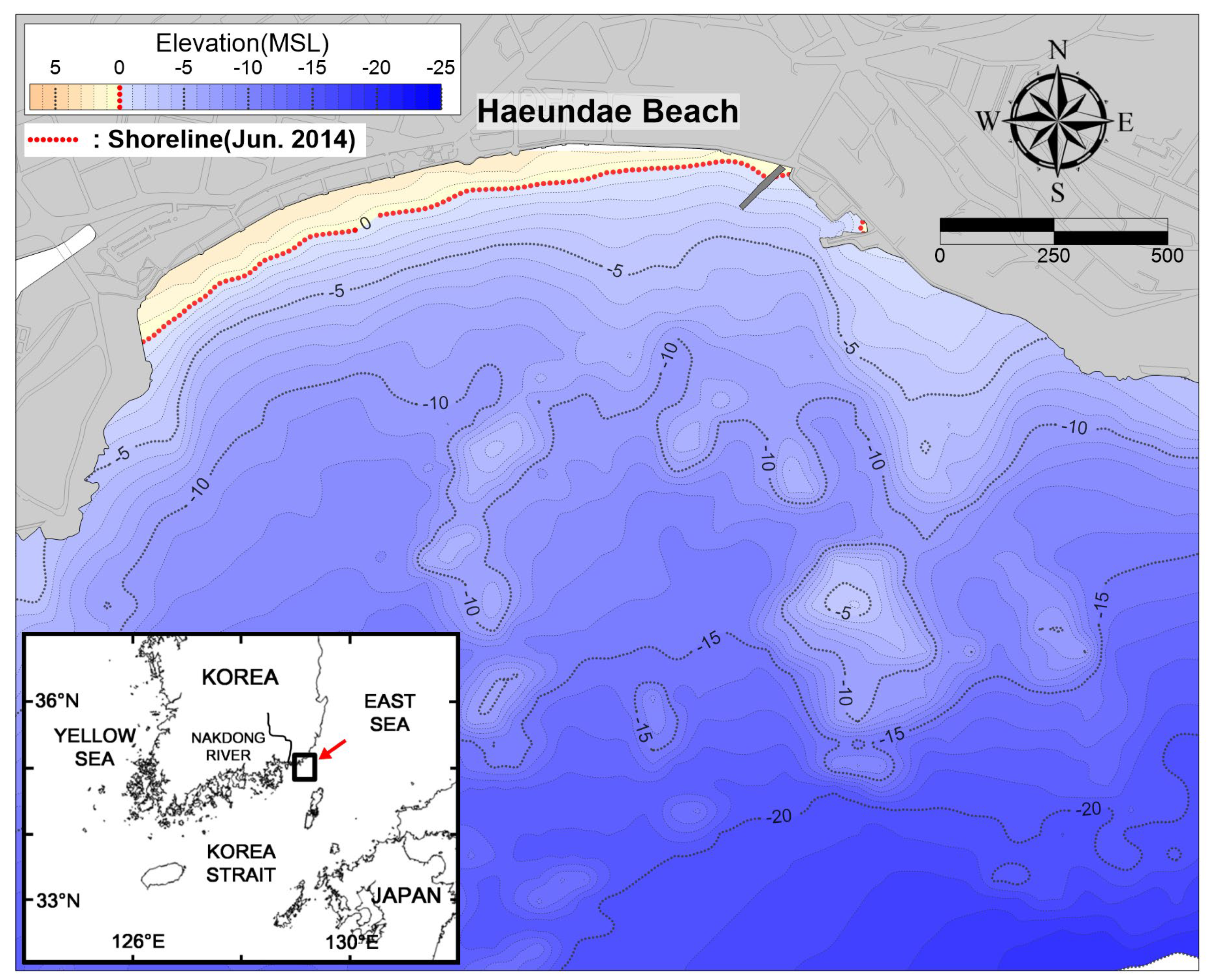
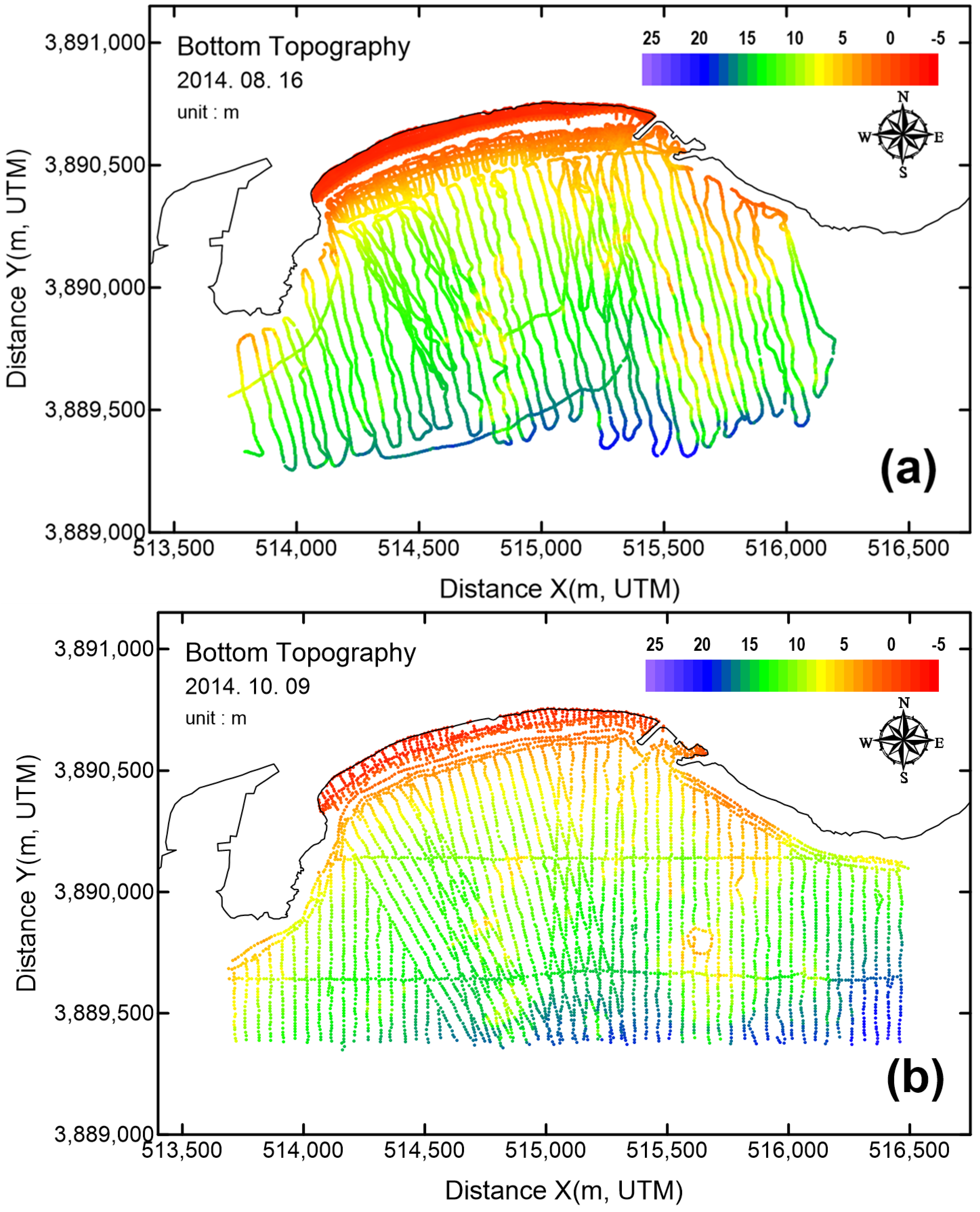
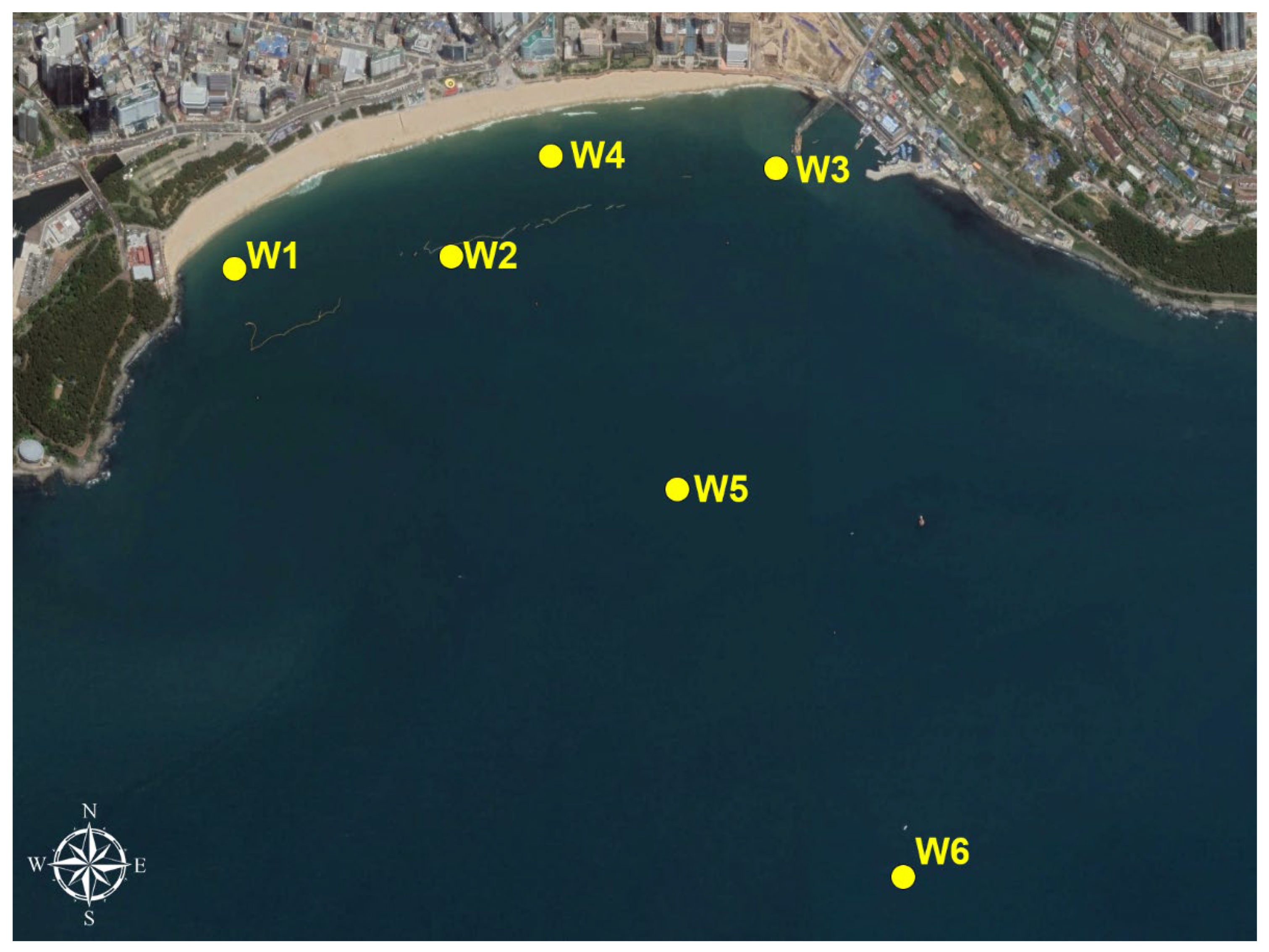
3.1. Field Observation

For the experimental site, we chose Haeundae Beach located in the southeast end of the Republic of Korea, where the tidal range was ~1.3 m (Figure 1). Haeundae Beach is one of the most popular beaches and millions of people visit annually. Due to its high value as a recreational area, Haeundae Beach has been protected by coastal structures and beach nourishment. In addition, scientific experiments have been conducted to monitor the hydrodynamic and sediment conditions in the area, which are available for the present study.
The field observation data used to validate the modeled data were obtained from two surveys conducted on 16 August and 9 October of 2014, measuring the water depths around the Haeundae Beach, Korea, as shown in Figure 2. The colored lines show the tracks of the boat that mounted a single-beam echosounder, and the line color marks the depth. Based on these survey data, a map of the morphological changes could be built between the two dates (Figure 3). One of the most significant changes can be found in the swash zone (z ~ 0 m, as identified in Figure 1) at the west end of the beach (marked as shape ‘A’ in Figure 3), where the bed level had been elevated as high as 1 m. Although not as clear as ‘A’, another area that shows accretion of the seabed is the east end of the swash zone of the beach (marked as shape ‘B’). While the seabed is accreted in the swash zone, it is generally eroded in the nearshore region widely in front of the beach (marked as shape ‘C’). In addition, many spotty locations that show severe seabed erosions (or depositions) are found in the deeper area (marked as shape ‘D’).
In addition to the bathymetry data, the wave data were also measured at six stations in the study site. Figure 4 shows the locations of the six wave measurement stations in the site. The time periods of the wave measurements were, however, different for each wave station. Unfortunately, no wave measurements were made for the whole period (16 August–9 October) to cover the time span between the two bathymetry measurements, as the longest-spanning wave data available were measured from 22 August to 21 September at the stations W4, W5, and W6. The conditions for the wave measurements at each wave station are listed in Table 1. The wave observation data were then compared with the numerical model data, and these results are described in Section 4.1.
Another important aspect of field data measured for this study was the measurement of the erodible bed thickness. As shown in Figure 3, spotty locations that exhibit severe seabed erosion and accretion were observed in the southeast area of the area (e.g., see circle ‘D’ in Figure 3), which is not clearly understood from the bathymetry data only. To examine this, additional field data were obtained by measuring erodible bed depths—i.e., the sand’s thickness over the rocks below it. The erodible bed depths were measured using the seismic reflection method (sending seismic waves into the ground and recording the reflections of these waves off subsurface interfaces) in May 2015 and the seismic refraction method (sending seismic waves into the ground at various angles and recording the time it takes for these waves to travel through different subsurface materials) in October 2015.
Figure 5 shows the distribution of the sand thickness. The thickness of the sand layer was greater than 5 m in most of the shallow areas of the beach, whereas the sand layer was thin in the areas in the eastern part of the beach where the water was, with depths between 5 m and 10 m. These thin sandy layers indicate that rocks were thickly developed below the sand, and these areas correspond to the spotty areas in Figure 3 where severe seabed erosions and accretions were observed in the southeast part of the beach. The measured sand thickness data were used as an input condition for the numerical experiments to consider the impact of the rocks in calculating the morphological changes, which will be discussed in Section 4.1.
The total observational period was from 16 August and 9 October of 2014, during which the bathymetry data were measured at each day and the wave measurements were available between the two end dates. It is also noted that Typhoon Phanfone, a category four cyclone, affiliated the Haeundae Beach area during the observational period, from October 2 to October 6. Therefore, it was expected that sediments in the beach face were actively transported in both the cross-shore and longshore directions during the corresponding period. One of the important characteristics of LW07 is that it can predict sediment transport in both cross-shore and longshore directions. Considering that a majority of the swash-zone models calculate only cross-shore transport, it is advantageous to apply LW07 to beaches where longshore transport is also dominant. The study site, Haeundae Beach, has been known to undergo active longshore sediment transport [43]. Therefore, we selected this site to examine the performance of LW07 with Telemac-2D. In addition, although this beach has been affiliated by many other storm wave events, including typhoons, the dataset used in this study comprised only the field observations that included bathymetry, topography, and hydrodynamic measurements before and after a severe storm event, which was advantageous for the model validation.

3.2. Numerical Model Setup

Based on the two bottom topography measurements that had a time difference of about two months, we designed the present numerical experiments. First, we built an unstructured grid system for the Telemac-2D modeling with 12,635 nodes and 24,660 elements based on the bathymetry data measured on 16 August of 2014, as shown in Figure 6. Inside the surf zone, the unstructured grids were refined to have the finest grid size, which was as small as 3 m. We then performed the numerical experiments by running the model for 55 days from 16 August to 9 October 2014.
The input and boundary conditions were determined from a larger-scale regional model that predicts the wave and tide conditions around the Korean peninsula using another Telemac-2D system. Figure 7 shows examples of this regional modeling system. In order to increase the accuracy of the prediction, the wind data obtained from the regional forecasting system (RDAPS) from the Korea Meteorological Administration were employed (Figure 7a).
For the model parameters, the time step was set as 2 s for the flow module and the waves calculated by Tomawac were incorporated into the flow module every 300 s. At the open boundary, the waves were generated using the Texel–Marsen–Arsloe (TMA) spectrum. The breaking of the waves was determined by the Thornton and Guza [44] equation. The sediment diameter (D50) used was 0.228 mm. One of the primary objectives of this study was to validate the Telemac-2D’s modeling performance by applying the Larson and Wamsley formula (LW07) in the swash zone. For this, LW07 was applied in the swash zone along the coast where the water depth is shallower than 2 m, as shown in Figure 8.
In the study site, the tidal range was ~1.3 m, and the foreshore, the part of shore between the high and low water levels in the tidal zone, was within the swash zone marked in Figure 8. The model calculated morphological changes only at the grid cells where the water depth was greater than zero, because the wave and flow modules were inactive at the grids where the seabed was not submerged beneath the water. During the tidal period, the number of grid cells submerged in the water varied according to changes in the sea level, consequently leading to continuous updates of the seabed levels in the foreshore area throughout the experimental period. In addition, the water depths of the grids located along the foreshore boundaries could be changed by adjusting the seabed levels of nearby cells, leading to changes in the topography of the foreshore zone.
During the model run period from 16 August to 9 October of 2014, Typhoon Phanfone affected the experimental site from 2 October to 6 October, when the category four cyclone passed the southwest part of the Korean peninsula. Unfortunately, hydrodynamic measurements were not available from any of the six wave stations during the typhoon period. The boundary conditions during the typhoon period could be still available from the regional model data calculated using wind fields from RDAPS (Figure 7a).

4. Results

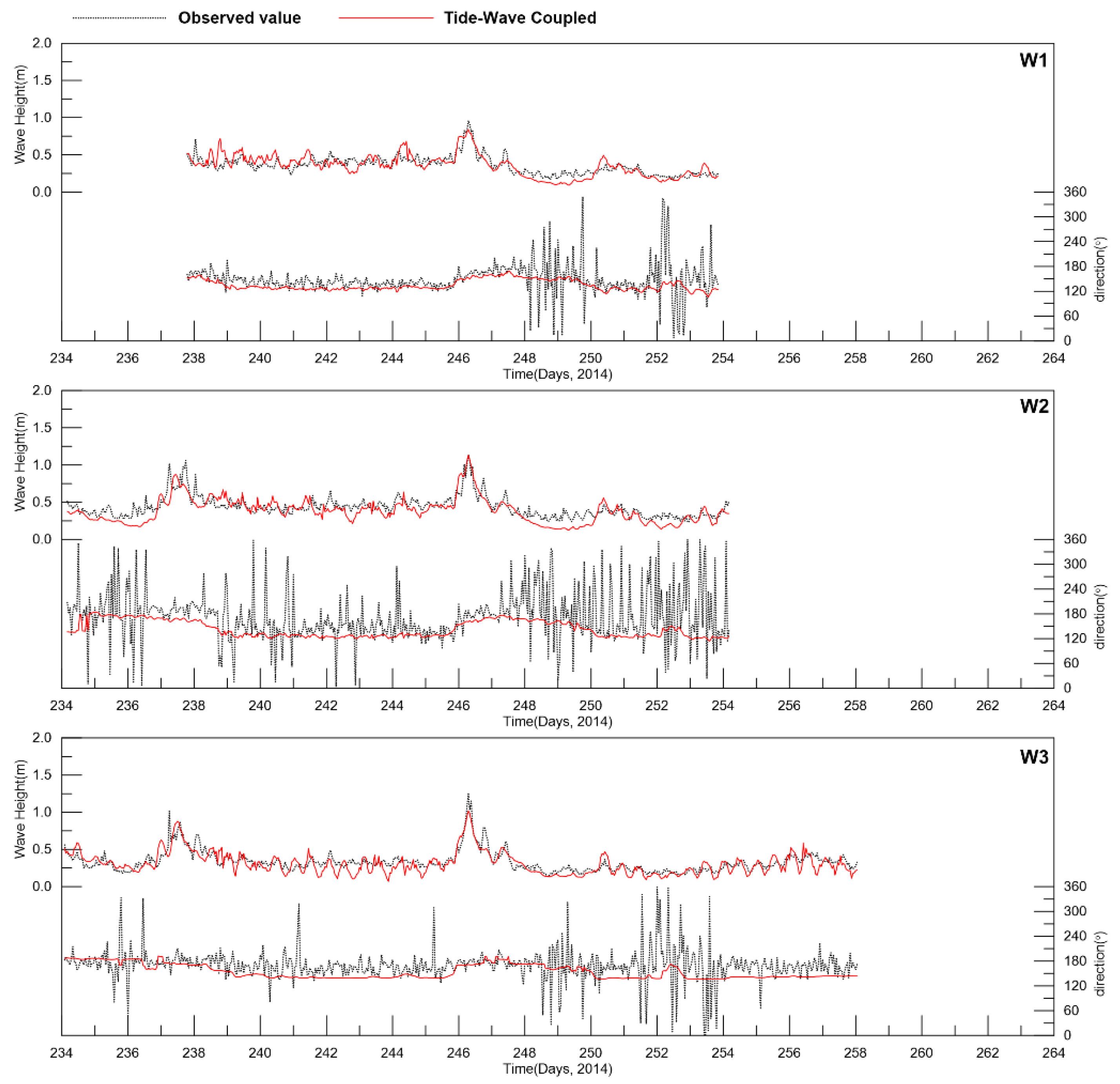
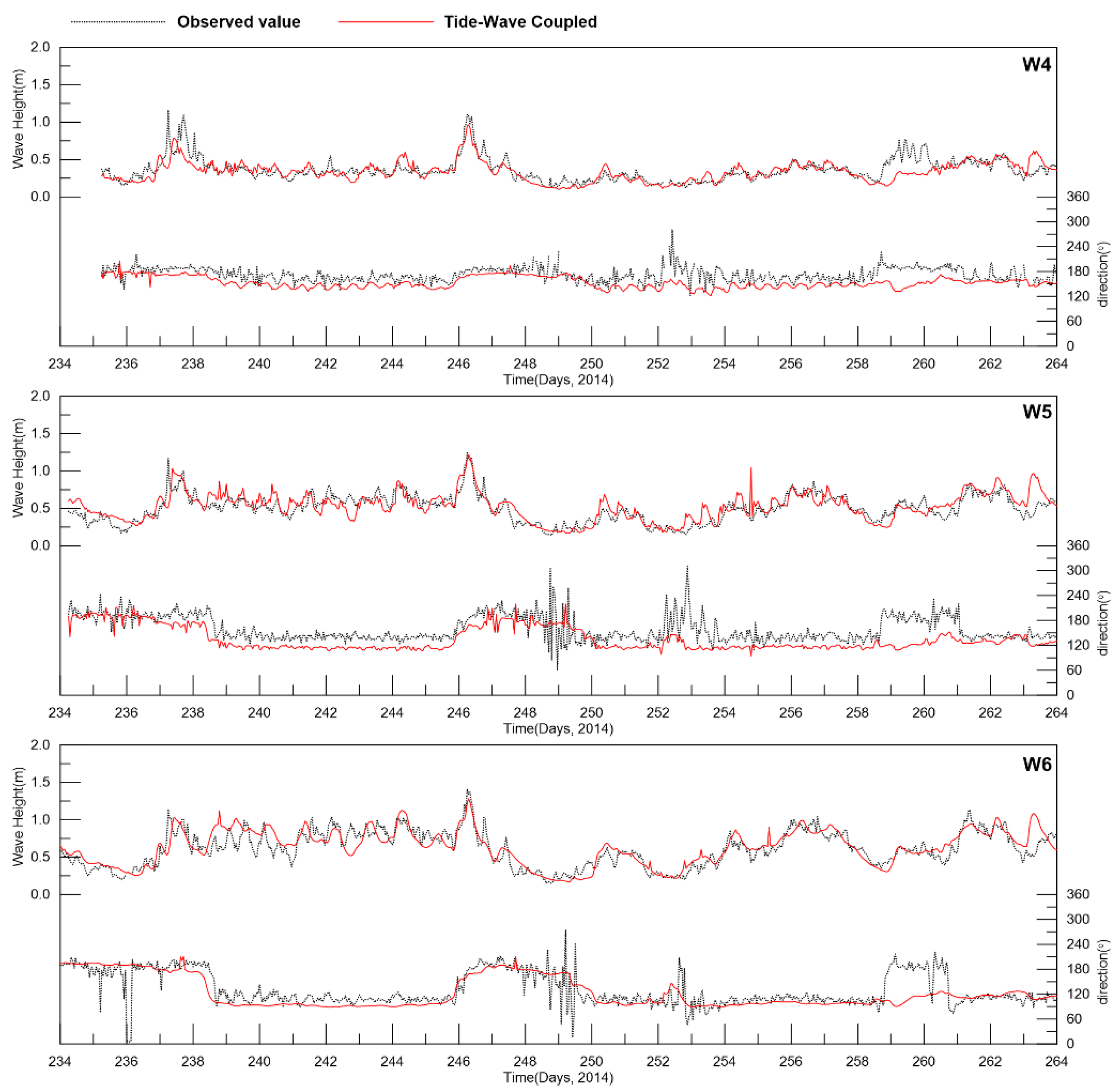
4.1. Model Validation

The observed and modeled wave heights (HS) and wave directions at the six stations are compared in Figure 9. The waves were nicely simulated by the model as the wave heights show generally good agreement between the model results and observations, except for unusual spikes observed in the observational data, especially in W1. For the wave directions, the comparison becomes more difficult because the observational data show severe fluctuations at most of the stations; these irregular deviations are likely due to observational error and thus are not able to be simulated by the model.
The wave conditions were generally mild during the period. The average wave height was lower than 1 m at all six stations. However, there were times when the observed as well as the modeled wave heights became higher than usual on 26 August and 3 September, wherein the observed maximum significant wave height reached 1.11 m and 1.41 m, respectively. The modeled maximum significant wave height was 1.02 m on August 26 and 1.28 m on September 3, showing reasonable agreement with errors with 8.8% and 10.1%, respectively. During the storm wave conditions caused by the Typhoon Phanfone, wave data were not observed at any of the six stations, so direct comparison was not available.
The next step for model validation was to examine the effect of the measured sand thickness distribution in Figure 5. As seen in Figure 3, the observational data of the morphological changes shows that spotty areas of strong erosions/depositions were measured in the southeastern part of the area. For example, Figure 10a shows a magnified view of the morphological changes during the observational period in the area focused around the red circle in Figure 5, showing that spotty locations of severe erosion and deposition were observed. However, these spotty locations could not be reflected in the model results when the model was run without the information of the measured sand thickness data. Figure 10b shows that the modeled morphological changes in the area were mostly uniform because the model considered the seabed to be covered by sand only. Therefore, the model was run again using the sand thickness data as input conditions. Figure 10c shows the results in which the spotty locations were successfully simulated in the corresponding area, compared to the results in Figure 10b, because the model knew that there were underwater rocks and the seabed over these rocky areas would not be eroded, while the sandy seabed could be eroded.

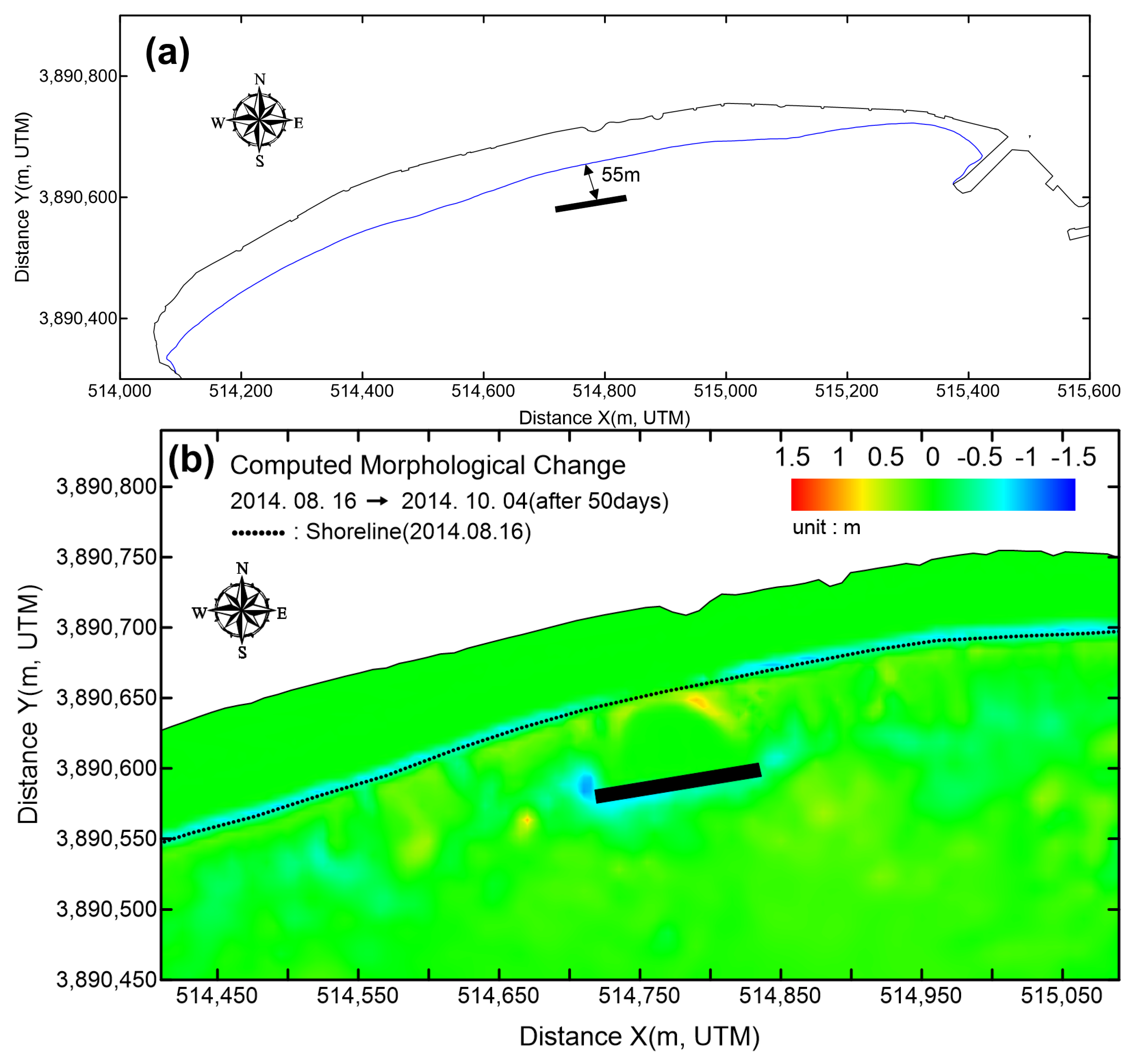
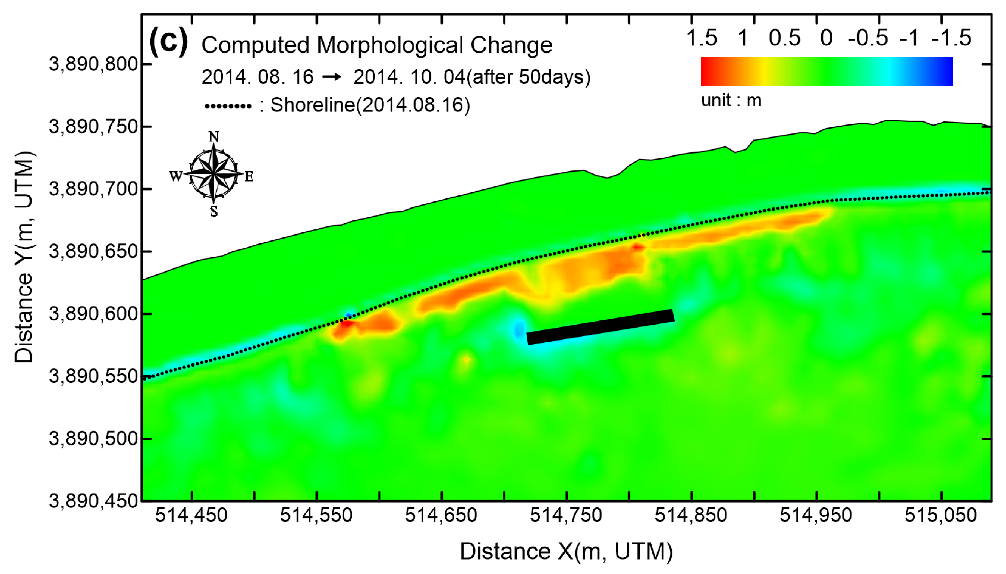
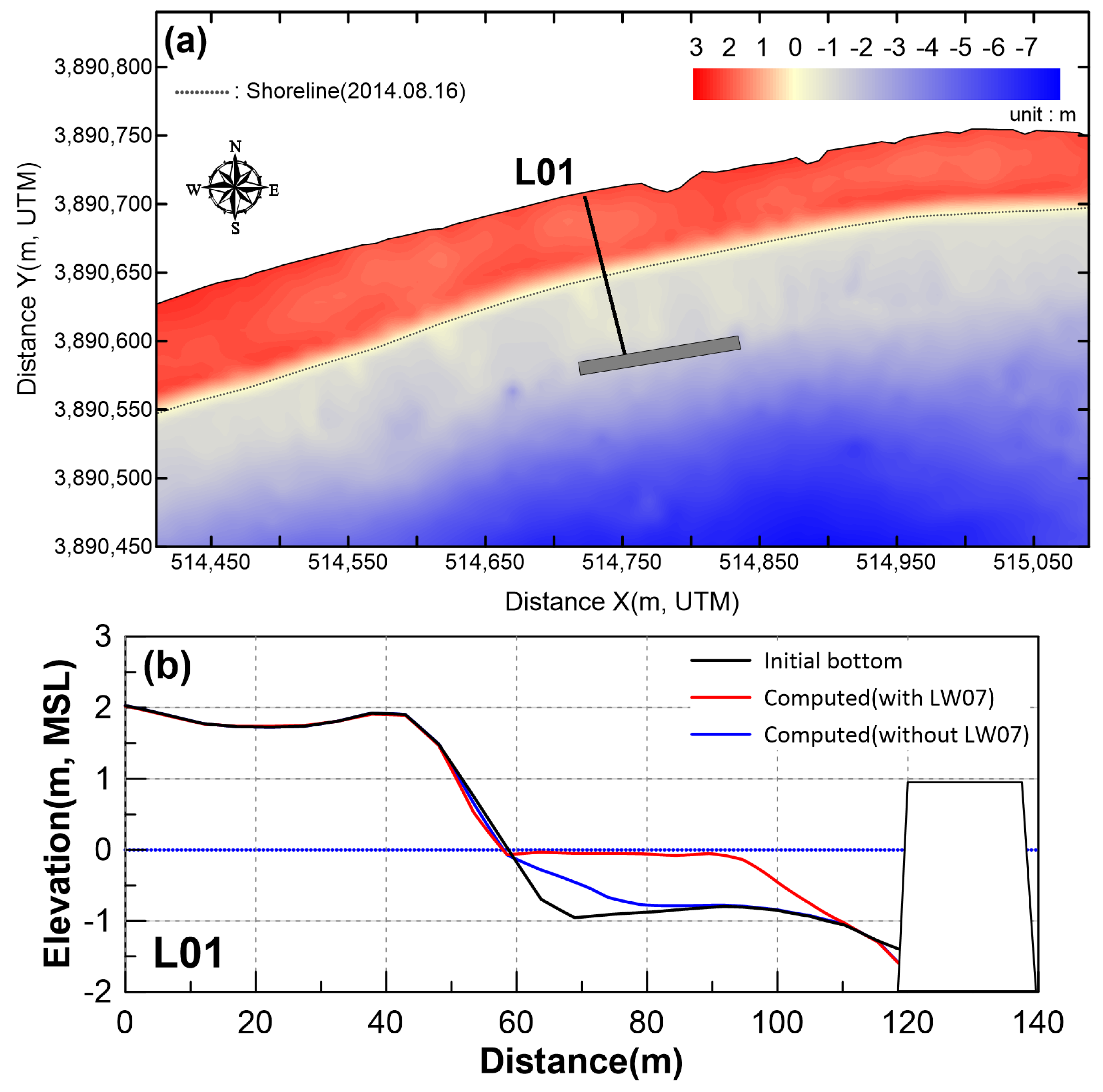
4.2. Morphological Changes—Test Case with Imaginary Breakwater

In this section, we performed a numerical experiment to test the validity of LW07 in modeling the swash-zone process. The purpose of this experiment was to examine the direct response of the swash-zone model to the shadowing of a coastal structure. For this, an imaginary breakwater was placed in the middle of the beach to run the model for 50 days from 16 August, and the result was compared with the results of running the model without the imaginary breakwater. The imaginary breakwater was 100 m long and located 55 m offshore from the coastline so that it could cause direct impact on the sediment transport pattern behind it (Figure 11a).
The results show a clear discrepancy between the two cases, as sediments considerably cumulated behind the breakwater in the case with the swash-zone formula (LW07) in the wide range along the shoreline behind the breakwater (~300 m), as shown in Figure 11c. In case without LW07, however, a smaller amount of sediments cumulated behind the breakwater (Figure 11b). In order to conduct a quantitative analysis, we drew a straight line (L01) from the beach to the imaginary breakwater, as shown in Figure 12a, and the profiles were compared between three cases: (1) the initial profile measured with field survey data; (2) the modeled profile with LW07 (the swash-zone formula); (3) the modeled profile without LW07 (Figure 12b). The results show that the modeled seabed location was elevated by a maximum of ~1.0 m when LW07 was applied, whereas the maximum seabed elevation was ~0.5 m without LW07. The range of seabed elevation along the profile also showed discrepancy because the seabed was elevated for ~150 m from the shoreline to offshore when the LW07 formula was applied, whereas this was ~90 m without LW07.
Although we do not have observational data to validate the model results, a rapid response of the shoreline to the breakwater was expected due to the shadowing of the waves that produces a sediment transport gradient along the shore behind the breakwater, considering the effect of costal structures observed in similar sites on the east coast of South Korea [45]. The results in Figure 11 and Figure 12 confirm that the seabed morphology around the shallow swash-zone area could be, at least, more significantly changed in the model results, responding to the construction of a breakwater, when the LW07 formula was applied.

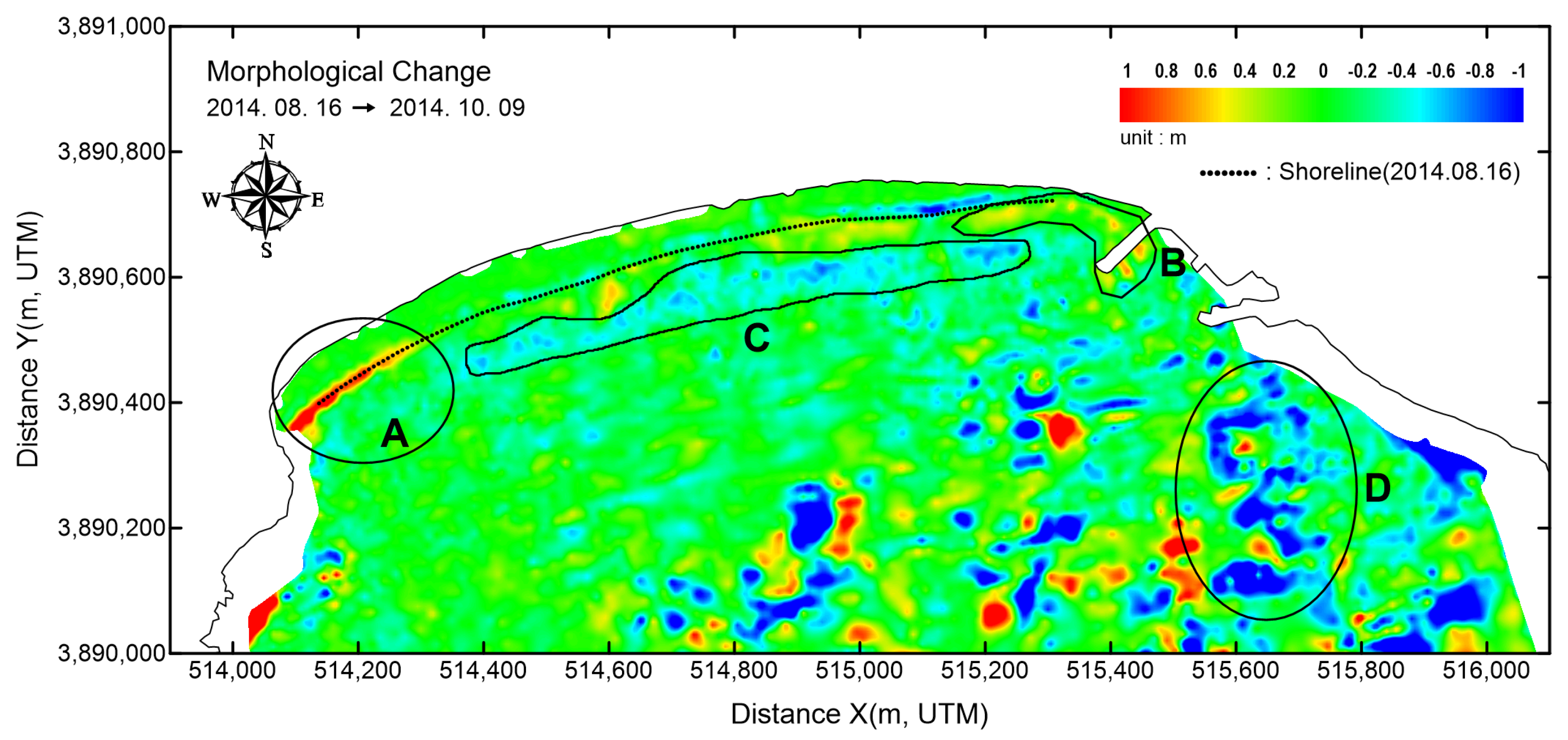
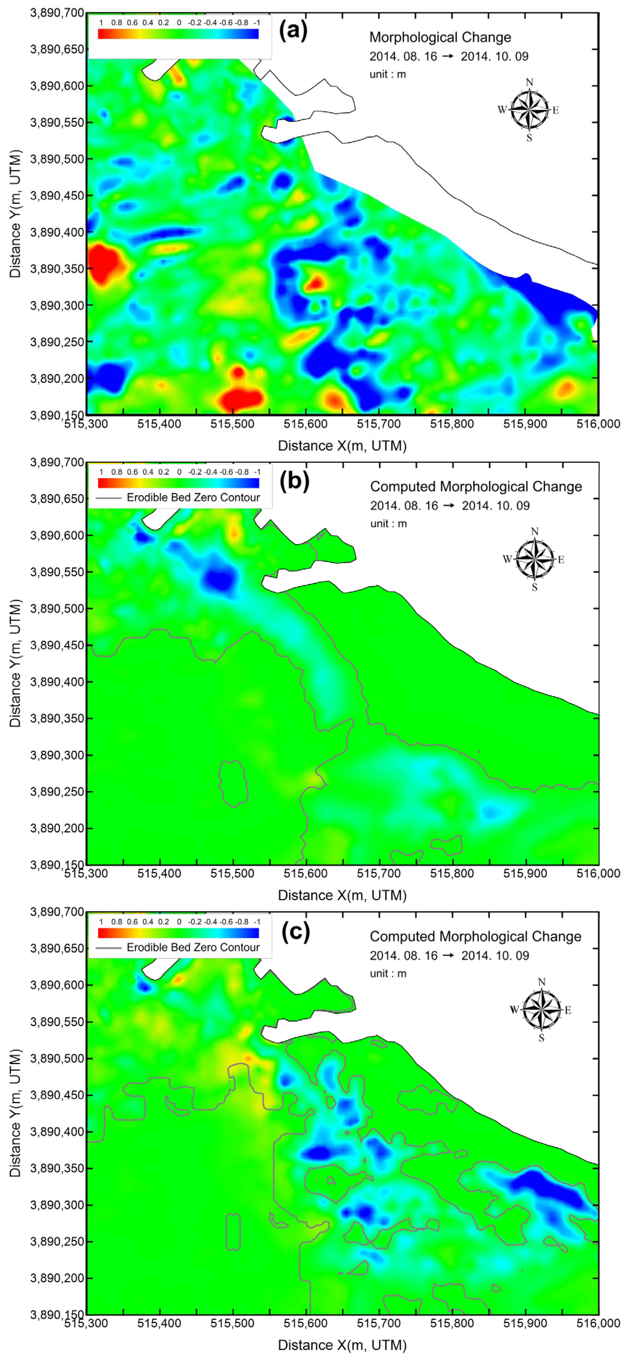
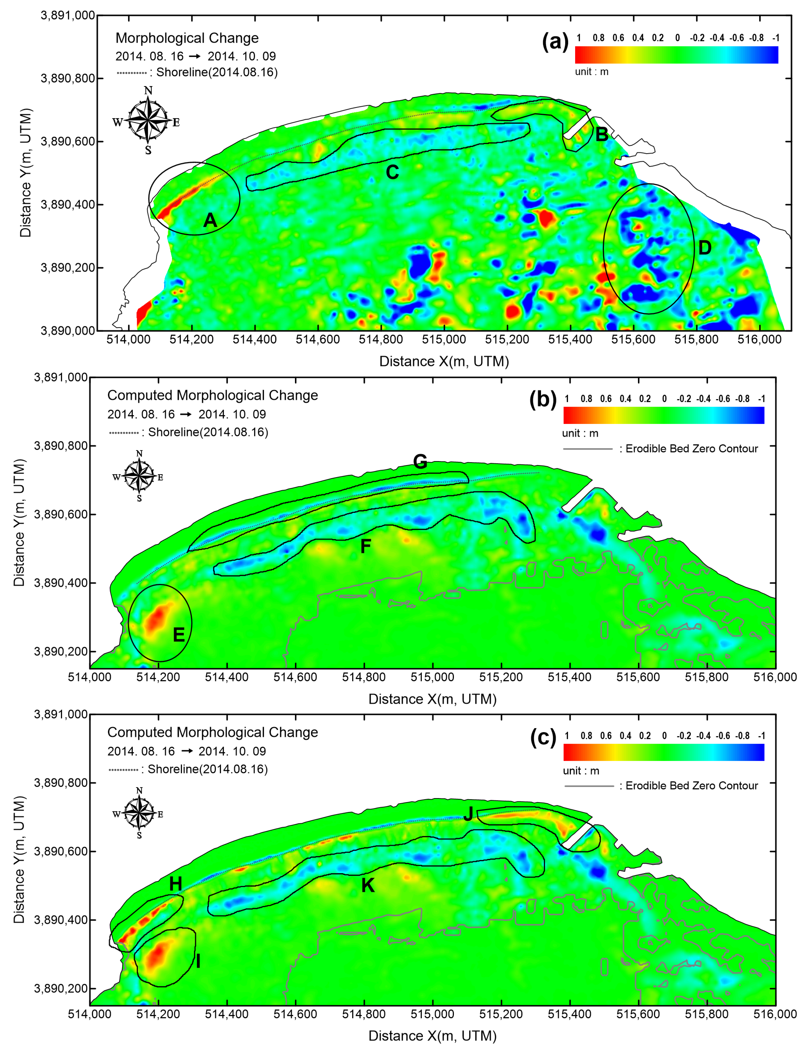
4.3. Morphological Change without LW07

In Section 4.3 and Section 4.4, the results of the modeled morphological changes in the study site are compared with the measured bathymetry data. The model was run in two cases by turning on/off LW07, the swash-zone formula. In order to compare the morphological changes measured in the field survey observations, the model was also run for 55 days from August 16 to October 9, corresponding to the dates of the field survey. Figure 13a shows the observation data of the seabed elevation changes between the two bathymetry measurements. It is noted that the distribution in Figure 13a is same as that in Figure 3; thus, the descriptions on the circled areas of ‘A’, ‘B’, ‘C’, and ‘D’ in the figure are not repeated in this section again and the readers are directed to Section 3.1.
In Figure 13b, the model results of morphological changes are shown for the case that was run after turning off LW07, the swash-zone formula. One of the characteristic features of the modeled data is that the observed sediment deposition in ‘A’ was not successfully simulated by the model. Instead, it showed that the modeled sediments cumulated in the deeper part of the nearshore region (circle ‘E’ in Figure 13b), which was not observed in the measured data. In addition, the seabed accretion in the east end of the swash zone (shape ‘B’ in Figure 13a) was not simulated by the model as well. Another failure of the model is found in the shape ‘G’. While the model predicted that the swash-zone area in ‘G’ had to have been eroded by about 0.5 m, the observational results in Figure 13a do not support this process, as they show no clear evidence of erosion in the corresponding swash area.
Although the model failed to predict the morphological changes in the swash zone, it showed reasonably good agreement in the deeper nearshore region. Both of the observational and model results show that the seabed was widely eroded in the nearshore area in front of the beach (shapes ‘C’ and ‘F’ in Figure 13a,b). The results show that the model without the swash-zone formula successfully simulated the coastal processes in the nearshore area outside the swash zone. However, the processes in the shallow swash zone were poorly simulated by the model, which suggests an additional engine may be required to properly control these swash-zone processes.

4.4. Morphological Changes with LW07

In this section, we discuss the model results of morphological changes with LW07 as its distribution, as shown in Figure 13c. The most significant improvement compared to the results without LW07 (Figure 13b) is the successful calculation of the sediment deposition observed in ‘A’, which was well simulated by the model with LW07, as emphasized in ‘H’ in Figure 13c. Another improved performance with LW07 is the successful simulation of the sediment deposition observed at the other end of beach’s swash zone (‘B’ in Figure 13a), as the model results also show deposition in the corresponding area (‘J’ in Figure 13c). Compared to when the model was run without LW07, the band of erosion along the swash zone in ‘G’ in Figure 13b was no longer simulated when it was run with LW07 (Figure 13c), which corresponds to the observational results as well (Figure 13a).
Outside the swash zone, the model results with LW07 were similar to those run without LW07. For example, the incorrect simulation of the seabed deposition in the west end of the nearshore area (‘E’ in Figure 13b) was also simulated in the run with LW07, as shown in ‘I’ in Figure 13c. In addition, the successful simulation of the erosion along the nearshore band (‘C’ in Figure 13a and ‘F’ in Figure 13b) was also repeated during the run with LW07, as shown in ‘K’ in Figure 13c. The results in this section confirm that the Telemac-2D modeling system equipped with the swash-zone formula showed improved performance in simulating morphological changes, specifically in the shallow swash zone.
In Table 2, the changes in the seabed morphology are compared quantitatively by calculating the changes in the seabed volume during the experimental period between the observational and modeled data, within the specified shapes marked in Figure 13a–c. It is found that the errors in the modeled data, compared with the observational data, were significantly reduced by applying LW07, although the errors in the modeled data with LW07 were still considerable, as they were within the range of 20~30%. The model’s accuracy in calculating the morphological changes is further discussed in the next section.

5. Discussion

In this section, we discuss the model results of morphological changes with LW07 as the model’s distribution, as shown in Figure 13c. The most significant improvement compared to the results without LW07 (Figure 13b) is seen in the successful calculation of the sediment deposition observed in ‘A’, which was simulated well by the model with LW07, as emphasized in ‘H’ in Figure 13c. Another improved aspect of performance with LW07 is the successful simulation of the sediment deposition observed at the other end of beach’s swash zone (‘B’ in Figure 13a), as the model results also show deposition in this corresponding area (‘J’ in Figure 13c). Compared to the run without LW07, the band of erosion along the swash zone in ‘G’ in Figure 13b was no longer simulated in the run with LW07 (Figure 13c), which corresponds to the observational results as well (Figure 13a).
Outside the swash zone, the model results with LW07 were similar to those run without LW07. For example, the incorrect simulation of the seabed deposition in the west end of the nearshore area (‘E’ in Figure 13b) was also simulated in the run with LW07, as shown in ‘I’ in Figure 13c. In addition, the successful simulation of the erosion along the nearshore band (‘C’ in Figure 13a and ‘F’ in Figure 13b) was also repeated during the run with LW07, as shown in ‘K’ in Figure 13c. The results in this section confirm that the Telemac-2D modeling system equipped with the swash-zone formula showed improved performance in simulating the morphological changes, specifically in the shallow swash zone.
The successful simulation results with LW07 could have been contributed to by the advantages of the formula, as shown in Equations (8) and (9). While a majority of swash-zone sand transport formulas are developed only for calculating cross-shore sediment transport [16], LW07 calculates longshore transport as well. As shown in Figure 13a, the observed morphological changes were dominant in the longshore direction in the swash zone, rather than the cross-shore direction. Therefore, this indicates that swash-zone formulas that predict only cross-shore transport could not be successful to simulate these longshore swash-zone sand transport processes, and LW07 might have advantage in calculating the longshore process over the cross-shore formulas in this specific case.
Although the pattern of morphological changes in the swash zone was successfully simulated by using LW07 when compared to the results after running the model without LW07, the results were not accurately simulated quantitatively. As shown in Table 2, the modeling errors in the morphological changes with LW07 were considerably high in the swash zone compared with the observations. The reasons for this inaccuracy could be various, but the limitations of the model were also obvious. Telemac-2D is based on a wave-averaged model, and complex wave dynamics in the swash zone like wave–swash interactions and run-up height are difficult to explicitly and accurately compute in the wave-averaged model [16]. In addition, the model does not consider the impact of long (infragravity frequency band) waves on the morphological changes. During storm events, infragravity swash would be also dominant and its energy could become strong enough to cause dune erosion [8]. The model in this study did not account for the impact of these infragravity-band waves, which might have lowered the modeling accuracy. Another disadvantage of LW07 is that the empirically determined coefficients, K c and K l , in Equations (8) and (9) were site-specific and required calibration for different beach conditions [16]. In this study, however, default values were used for these coefficients, which also might have contributed to the errors.
These limitations that might cause modeling errors need to be considered in designing future studies. It is also noted that an updated version of the bedload formula was proposed by Zhang and Larson [46], by which the effect of velocity asymmetry was considered in estimating the net transport. Considering the possible contribution of asymmetry to net sand transport in the swash zone, it is recommended to apply this formula to be combined with Telemac-2D or another 2DH model to examine its performance for future studies.

6. Conclusions

In this study, the performance of the Larson and Wamsley [1] swash-zone formula was examined in Haeundae Beach, Korea, where many scientific observations have been made to monitor this most popular beach. For numerical experiments, we employed the Telemac-2D model system to calculate the hydrodynamics and the consequent morphological changes from 16 August and 9 October of 2014, during which the category four Typhoon Phanfone affected the experimental site from 2 October to 6 October. During this period, we observed that the seabed elevation was significantly changed at both ends of the swash zone of the beach, where it was accreted up to 1 m, while the nearshore area in the middle of the beach was eroded up to 0.6 m. The model was validated with observational wave and current data measured at six stations. In addition, the model’s performance was enhanced by employing the measure erodible bed thickness in the area where under-seabed rocks were abundantly distributed.
The results showed that the model successfully simulated the erosion in the nearshore region, whether the swash-zone formula was used or not. However, the model failed to simulate the swash-zone process if LW07 was not employed. The observed seabed accretion at both ends of the beach swash zone was only successfully simulated if LW07 was used. The swash-zone formula also worked nicely to simulate the shoreline’s response to a coastal breakwater. The better performance achieved when using LW07 in modeling swash-zone processes might be due to the adjustment of the local beach slope that played a role in mitigating severe erosion/accretion processes in the swash zone. Due to the importance of correct prediction of swash-zone processes in coastal modeling, further exploration is required to enhance the performance of swash-zone models through comparing their results with field observations.

Author Contributions

Conceptualization, J.D.D., J.-Y.J., W.-M.J. and Y.S.C.; methodology, J.D.D., B.L. and S.K.H.; software, J.D.D. and S.K.H.; investigation, J.D.D., B.L. and S.K.H.; resources, J.-Y.J. and W.-M.J.; data curation, J.D.D. and B.L.; writing—original draft preparation, J.D.D. and Y.S.C.; writing—review and editing, Y.S.C.; visualization, J.D.D. and B.L.; supervision, J.-Y.J., W.-M.J. and Y.S.C.; project administration, J.D.D.; funding acquisition, J.D.D. and Y.S.C. All authors have read and agreed to the published version of the manuscript.

Funding

This research was funded by the Korea Institute of Ocean Science and Technology (grant number: PEA0205).

Data Availability Statement

The data presented in this study are available on request from the corresponding author. The data are not publicly available due to big size data.

Conflicts of Interest

Author Sang Kwon Hyun is employed by Sekwang Engineering Consultants Company Limited. The remaining authors declare that this research was conducted in the absence of any commercial or financial relationships that could be construed as a potential conflict of interest.

References

  1. Pelnard-Considère, R. Essai de theorie de l’evolution des formes de rivage en plages de sable et de galets. Journées De L’hydraulique 1957, 4, 289–298. [Google Scholar]
  2. Ruggiero, P.; Buijsman, M.; Kaminsky, G.M.; Gelfenbaum, G. Modeling the effects of wave climate and sediment supply variability on large-scale shoreline change. Mar. Geol. 2010, 273, 127–140. [Google Scholar] [CrossRef]
  3. Chang, Y.S.; Huisman, B.; De Boer, W.; Yoo, J. Hindcast of Long-term Shoreline Change due to Coastal Interventions at Namhangjin, Korea. J. Coast. Res. 2018, 85, 201–205. [Google Scholar] [CrossRef]
  4. Drønen, N.; Deigaard, R. Quasi-three-dimensional modelling of the morphology of longshore bars. Coast. Eng. 2007, 54, 197–215. [Google Scholar] [CrossRef]
  5. Militello, A.; Reed, C.W.; Zundel, A.K.; Kraus, N.C. Two-Dimensional Depth-Averaged Circulation Model M2D: Version 2.0, Report 1, Technical Documentation and User’s Guide; U.S. Army Engineer Research and Development Center: Vicksburg, MS, USA; Washington, DC, USA, 2004. [Google Scholar]
  6. Buttolph, A.M.; Kraus, N.C.; Wamsley, T.V. Two-Dimensional Depth-Averaged Circulation Model CMS-M2D: Version 3.0. Sediment Transport and Morphology Change. Report 2; U.S. Army Engineer Research and Development Center: Vicksburg, MS, USA; Washington, DC, USA, 2006. [Google Scholar]
  7. Bruneau, N.; Bonneton, P.; Pedreros, R.; Dumas, F.; Idier, D. A new morphodynamic modelling platform: Application to characteristic sandy systems of the Aquitanian Coast, France. J. Coast. Res. 2007, 50, 932–936. Available online: https://www.jstor.org/stable/26481716 (accessed on 10 March 2024).
  8. Roelvink, D.; Reniers, A.; Van Dongeren, A.; De Vries, J.V.T.; McCall, R.; Lescinski, J. Modelling storm impacts on beaches, dunes and barrier islands. Coast. Eng. 2009, 56, 1133–1152. [Google Scholar] [CrossRef]
  9. Nam, P.T.; Larson, M.; Hanson, H. A numerical model of nearshore waves, currents, and sediment transport. Coast. Eng. 2009, 56, 1084–1096. [Google Scholar] [CrossRef]
  10. Nam, P.T.; Larson, M.; Hanson, H. Modeling morphological evolution in the vicinity of coastal structures. In Proceedings of the ASCE 32nd International Conference on Coastal Engineering, Shanghai, China, 6 February 2011. [Google Scholar]
  11. Nam, P.T.; Larson, M. Model of nearshore waves and wave-induced currents around a detached breakwater. J. Waterw. Port Coast. Ocean Eng. 2010, 136, 156–176. [Google Scholar] [CrossRef]
  12. Nam, P.T.; Larson, M.; Hanson, H. A numerical model of beach morphological evolution due to waves and currents in the vicinity of coastal structures. Coast. Eng. 2011, 58, 863–876. [Google Scholar] [CrossRef]
  13. Baykal, C.; Ergin, A.; Güler, I. Two-dimensional depth-averaged beach evolution modeling: Case study of the Kızılırmak River mouth, Turkey. J. Waterw. Port Coast. Ocean Eng. 2014, 140, 05014001. [Google Scholar] [CrossRef]
  14. Karambas, T.V.; Samaras, A.G. An integrated numerical model for the design of coastal protection structures. J. Mar. Sci. Eng. 2017, 5, 50. [Google Scholar] [CrossRef]
  15. Hermawan, S.; Bangguna, D.; Mihardja, E.; Fernaldi, J.; Prajogo, J.E. The hydrodynamic model application for future coastal zone development in remote area. Civ. Eng. J. 2023, 9, 1828–1850. [Google Scholar] [CrossRef]
  16. Chen, W.; Van Der Werf, J.; Hulscher, S. A review of practical models of sand transport in the swash zone. Earth Sci. Rev. 2023, 238, 104355. [Google Scholar] [CrossRef]
  17. Larson, M.; Wamsley, T.V. A formula for longshore sediment transport in the swash. In Coastal Sediments’ 07; American Society of Civil Engineers (ASCE): New Orleans, LA, USA, 2007; pp. 1924–1937. [Google Scholar]
  18. Villaret, C.; Hervouet, J.-M.; Kopmann, R.; Merkel, U.; Davies, A.G. Morphodynamic modeling using the Telemac finite-element system. Comput. Geosci. 2013, 53, 105–113. [Google Scholar] [CrossRef]
  19. Larson, M.; Kubota, S.; Erikson, L. Swash-zone sediment transport and foreshore evolution: Field experiments and mathematical modeling. Mar. Geol. 2004, 212, 61–79. [Google Scholar] [CrossRef]
  20. Madsen, O. Sediment Transport on the Shelf, in ‘Sediment Transport Workshop Proc; DRP TA1; CERC: Vicksburg, MI, USA, 1993. [Google Scholar]
  21. Hervouet, J.M. A high resolution 2-D dam-break model using parallelization. Hydrol. Process. 2000, 14, 2211–2230. [Google Scholar] [CrossRef]
  22. Hervouet, J.-M. Hydrodynamics of Free Surface Flows: Modelling with the Finite Element Method; John Wiley & Sons: Hoboken, NJ, USA, 2007. [Google Scholar]
  23. Do, J.D.; Jin, J.-Y.; Hyun, S.K.; Jeong, W.M.; Chang, Y.S. Numerical investigation of the effect of wave diffraction on beach erosion/accretion at the Gangneung Harbor, Korea. J. Hydro-Environ. Res. 2020, 29, 31–44. [Google Scholar] [CrossRef]
  24. Do, J.-D.; Hyun, S.-K.; Jin, J.-Y.; Lee, B.; Jeong, W.-M.; Ryu, K.-H.; Back, W.-D.; Choi, J.-H.; Chang, Y.S. Wave Transformation behind a Breakwater in Jukbyeon Port, Korea—A Comparison of TOMAWAC and ARTEMIS of the TELEMAC System. J. Mar. Sci. Eng. 2022, 10, 2032. [Google Scholar] [CrossRef]
  25. EDF-R&D. TELEMAC Modelling System. 2D Hydrodynamics TELEMAC-2D Software Release 7.0 USER MANUAL; EDF R&D: Orvanne, France, 2014. [Google Scholar]
  26. EDF-R&D. Sisyphe v6.3 User’s Manual; EDF R&D: Orvanne, France, 2014. [Google Scholar]
  27. EDF-R&D. TELEMAC Modelling System. TOMAWAC Software. Release 7.1 OPERATING MANUAL; EDF R&D: Orvanne, France, 2016. [Google Scholar]
  28. Asaro, G.; Paris, E. The effects induced by a new embankment at the confluence between two rivers: TELEMAC results compared with a physical model. Hydrol. Process. 2000, 14, 2345–2353. [Google Scholar] [CrossRef]
  29. Giardino, A.; Ibrahim, E.; Adam, S.; Toorman, E.A.; Monbaliu, J. Hydrodynamics and cohesive sediment transport in the Ijzer estuary, Belgium: Case study. J. Waterw. Port Coast. Ocean Eng. 2009, 135, 176–184. [Google Scholar] [CrossRef]
  30. Robins, P.E.; Davies, A.G. Application of TELEMAC-2D and SISYPHE to complex estuarine regions to inform future management decisions. XVIIIth Telemac Mascaret User Club 2011, 19, 86. [Google Scholar]
  31. Benoit, M.; Marcos, F.; Becq, F. Development of a third generation shallow-water wave model with unstructured spatial meshing. In Coastal Engineering 1996; American Society of Civil Engineers: Reston, VA, USA, 1997; pp. 465–478. [Google Scholar]
  32. Nicolle, A.; Karpytchev, M.; Benoit, M. Amplification of the storm surges in shallow waters of the Pertuis Charentais (Bay of Biscay, France). Ocean Dyn. 2009, 59, 921–935. [Google Scholar] [CrossRef]
  33. Nairn, R.B.; Roelvink, J.; Southgate, H.N. Transition zone width and implications for modelling surfzone hydrodynamics. Coast. Eng. 1990, 1990, 68–81. [Google Scholar]
  34. Neessen, K.C. Analysing Depth-Dependence of Cross-Shore Mean-Flow Dynamics in the Surf Zone. Master’s Thesis, University of Twente, Enschede, The Netherlands, 2012. [Google Scholar]
  35. Svendsen, I.A. Wave heights and set-up in a surf zone. Coast. Eng. 1984, 8, 303–329. [Google Scholar] [CrossRef]
  36. Longuet-Higgins, M.S.; Stewart, R. Radiation stresses in water waves; a physical discussion, with applications. In Proceedings of the Deep Sea Research and Oceanographic Abstracts; Elsevier: Amsterdam, The Netherlands, 1964; pp. 529–562. [Google Scholar]
  37. Madsen, O.; Wright, L.; Boon, J.; Chisholm, T. Wind stress, bed roughness and sediment suspension on the inner shelf during an extreme storm event. Cont. Shelf Res. 1993, 13, 1303–1324. [Google Scholar] [CrossRef]
  38. Larson, M.; Camenen, B.; Nam, P.T. A unified sediment transport model for inlet application. J. Coast. Res. 2011, 59, 27–38. [Google Scholar] [CrossRef]
  39. Camenen, B.; Larson, M. A general formula for non-cohesive bed load sediment transport. Estuar. Coast. Shelf Sci. 2005, 63, 249–260. [Google Scholar] [CrossRef]
  40. Camenen, B. A Unified Sediment Transport Formulation for Coastal Inlet Application; US Army Engineer Research and Development Center: Vicksburg, MS, USA, 2007. [Google Scholar]
  41. Camenen, B.; Larson, M. A general formula for noncohesive suspended sediment transport. J. Coast. Res. 2008, 24, 615–627. [Google Scholar] [CrossRef]
  42. Hunt Jr, I.A. Design of seawalls and breakwaters. J. Waterw. Harb. Div. 1959, 85, 123–152. [Google Scholar] [CrossRef]
  43. Lee, H.J.; Do, J.-D.; Kim, S.S.; Park, W.-K.; Jun, K. Haeundae Beach in Korea: Seasonal-to-decadal wave statistics and impulsive beach responses to typhoons. Ocean Sci. J. 2016, 51, 681–694. [Google Scholar] [CrossRef]
  44. Thornton, E.B.; Guza, R. Transformation of wave height distribution. J. Geophys. Res. Ocean. 1983, 88, 5925–5938. [Google Scholar] [CrossRef]
  45. Do, J.D.; Jin, J.-Y.; Jeong, W.M.; Lee, B.; Choi, J.Y.; Chang, Y.S. Collapse of a coastal revetment due to the combined effect of anthropogenic and natural disturbances. Sustainability 2021, 13, 3712. [Google Scholar] [CrossRef]
  46. Zhang, J.; Larson, M. A numerical model for offshore mound evolution. J. Mar. Sci. Eng. 2020, 8, 160. [Google Scholar] [CrossRef]
Figure 1. Location of Haeundae Beach and the bottom topography around it. The red dotted line marks the position of the shoreline. The tidal range of the beach was ~1.3 m.
Water 16 00836 g001
Figure 2. Survey map for the depth measurement in the Haeundae Beach conducted on (a) 16 August and (b) 9 October 2014. These survey data were used to build the bottom topography map shown in Figure 1.
Water 16 00836 g002
Figure 3. Morphological changes between August 16 and October 9 of 2014 calculated based on the survey data observed on the corresponding dates. The circles ‘A’, ‘B’, ‘C’, and ‘D’ mark the areas with significant seabed accretion and erosion. The black dotted line marks the position of the shoreline.
Water 16 00836 g003
Figure 4. Satellite image showing the locations of the six stations (W1–W6) where the wave and tide data were measured at different points during 22 August–21 September 2014 (see Table 1 for the wave measurement period at each station).
Water 16 00836 g004
Figure 5. Map of the measured erodible bed thickness (i.e., the sand’s thickness over the rocks below it). Inside the red circle, a thin sand layer over the rocks is shown, corresponding to the complicated distribution of the erosional and accretional spotty areas in circle ‘D’ shown in Figure 3. The black dotted line marks the position of the shoreline.
Water 16 00836 g005
Figure 6. Unstructured grid system for the Telemac-2D modeling with 12,635 nodes and 24,660 elements based on the bathymetry data measured on 16 August 2014. Inside the surf zone, the unstructured grids were refined to have the finest grid size, as small as 3 m.
Water 16 00836 g006
Figure 7. Examples from the Telemac-2D regional model that is currently running to predict waves and tides around the Korean peninsula. The outputs of the regional model were used to compute the input and boundary conditions of our Haeundae Beach model. (a) Wind data obtained from the regional forecasting system (RDAPS) from the Korea Meteorological Administration. (b) An example of a calculated wave field.
Water 16 00836 g007
Figure 8. The area (blue color) where the Larson and Wamsley (2007) swash-zone formula applied [17].
Water 16 00836 g008
Figure 9. Comparison of wave height and direction between observational and modeled data at the six wave stations (W1W6). The comparison period is different for each wave station according to the times of observation.
Water 16 00836 g009aWater 16 00836 g009b
Figure 10. Comparison of morphological changes in a focused area of the southeastern part of the Haeundae Beach (the area around the red circle in Figure 5). (a) Observation; (b) model results without sand thickness data; (c) model results with sand thickness data. This shows that the spotty locations with severe seabed erosion could be successfully simulated when the measured sand thickness data were applied.
Water 16 00836 g010
Figure 11. (a) Location of the imaginary breakwater placed in the computational domain. (b) Model result of morphological change in 50 days from 16 August 2014, after being run without LW07. (c) Model result of morphological change in 50 days from 16 August 2014, after being run with LW07. The black dotted line marks the position of the shoreline.
Water 16 00836 g011aWater 16 00836 g011b
Figure 12. (a) Location of the straight line (L01) that connects the beach end and the imaginary breakwater. The black dotted line marks the position of the shoreline. (b) Comparison of the beach profiles along L01 between the two model results, with and without LW07—black: initial profile measured in the survey on 16 August; red: modeled profile with LW07; blue: modeled profile without LW07. The blue dotted line marks the position of the water level (mean sea level).
Water 16 00836 g012
Figure 13. Comparison of morphological changes between the model results without and with LW07. (a) Observation (16 August–9 October); (b) modeled results without LW07 (16 August–9 October); (c) modeled results with LW07 (16 August–9 October).
Water 16 00836 g013
Table 1. Instruments and data sampling parameters.
InstrumentsObservation PeriodBurst IntervalSampling Rate and Number of Samples Per Burst
St. W1ADCP 1200 kHz16 days
(1)
Wave: 3600 s
(2)
Current: 1800 s
(1)
Wave:
2 Hz and 2400
(2)
Current:
2 Hz and 1200
St. W2ADCP 1200 kHz20 days
St. W3ADCP 1200 kHz24 days
St. W4AWAC 1000 kHz30 days
St. W5AWAC 500 kHz30 days
St. W6AWAC 500 kHz30 days
Table 2. Morphological changes in the seabed volume during the experimental period within the specified shapes marked in Figure 13: (a) calculated from observational data, (b) calculated from modeled data run without LW07, (c) calculated from modeled data run with LW07. It is noted that the shape ‘H’ is identical to ‘A’, as is ‘J’ to ‘B’; ‘K’ to ‘C’ and ‘F’; and ‘I’ to ‘E’.
Section(a) Observation (m3)(b) without LW07 (m3)(c) with LW07 (m3)
D−16,910−13,936−13,514
G−4167−8489−5269
H (A)4767−3233372
I (E)113552584962
J (B)2344−123652
K (C, F)−8164−13,974−12,443
Disclaimer/Publisher’s Note: The statements, opinions and data contained in all publications are solely those of the individual author(s) and contributor(s) and not of MDPI and/or the editor(s). MDPI and/or the editor(s) disclaim responsibility for any injury to people or property resulting from any ideas, methods, instructions or products referred to in the content.

