Article

Assessing Future Hydrological Variability in a Semi-Arid Mediterranean Basin: Soil and Water Assessment Tool Model Projections under Shared Socioeconomic Pathways Climate Scenarios

by
Marziyeh Haji Mohammadi
1,
Vahid Shafaie
2,
Aliakbar Nazari Samani
1,
Arash Zare Garizi
3 and
Majid Movahedi Rad
2,*
1
Faculty of Natural Resources, University of Tehran, Karaj 31587, Iran
2
Department of Structural and Geotechnical Engineering, Széchenyi István University, 9026 Győr, Hungary
3
Faculty of Rangeland and Watershed Management, Gorgan University of Agricultural Sciences and Natural Resources, Gorgan 49138, Iran
*
Author to whom correspondence should be addressed.
Water 2024, 16(6), 805; https://doi.org/10.3390/w16060805
Submission received: 2 February 2024 / Revised: 4 March 2024 / Accepted: 6 March 2024 / Published: 8 March 2024
(This article belongs to the Section Hydrology)

Abstract

:
Climate is one of the main drivers of hydrological processes, and climate change has caused worldwide effects such as water scarcity, frequent floods and intense droughts. The purpose of this study was to analyze the effects of climate change on the water balance components, high flow and low flow stream conditions in a semi-arid basin in Iran. For this reason, the climate outputs of the CanESM5 model under Shared Socioeconomic Pathways (SSP) scenarios SSP126, SSP245, and SSP585 were spatially downscaled by the Statistical Downscaling Model (SDSM). The hydrological process was simulated by the Soil and Water Assessment Tool (SWAT) model. Key findings include a 74% increase in evapotranspiration, a reduction by up to 9.6% in surface runoff, and variations in discharge by up to 53.6%. The temporal analysis of snow melting changes revealed an increase in the volume of snow melting during winter months and a reduction in the volume during spring. The projected climate change is expected to cause notable variations in high and low flow events, particularly under the SSP585 scenario, which anticipates significant peaks in flow rates. This comprehensive analysis underscores the pressing need for adaptive strategies in water resource management to mitigate the anticipated impacts of climate variability.

1. Introduction

Climate change is anticipated to significantly amplify the hydrological cycle, thereby heightening the risks associated with floods and droughts in the foreseeable future [1,2,3,4]. This phenomenon, driven by alterations in temperature and precipitation patterns, has expedited changes in water balance components, consequently impacting riverine water resources [5]. Such climatic shifts are poised to influence seasonal streamflow patterns, inducing interannual fluctuations in hydrological processes [6]. The temperature variations attributed to anthropogenic activities are known to induce climate variability, which in turn affects the availability of surface and groundwater. This outcome is facilitated by modifications in atmospheric humidity, planetary rotation, precipitation patterns, soil moisture retention capabilities, and runoff, ultimately accelerating alterations within a catchment area’s water cycle by enhancing evaporation rates [7,8]. The Sixth Assessment Report (AR6) of the Intergovernmental Panel on Climate Change (IPCC) highlights that climate change has a disproportionate impact on societies with limited adaptation capabilities, particularly in developing countries characterized by rapid population growth and underdeveloped social and economic structures [9]. Given these considerations, a detailed examination of streamflow variations becomes imperative for effective water resource management within river basins, aiming to mitigate the risks of floods and droughts while averting significant adverse impacts on societal structures and environmental integrity [10].
The Global Climate Model (GCM) is a vital tool in predicting potential future climate change. The latest GCMs were developed by the World Climate Research Program (WCRP) as part of the Sixth Coupled Model Intercomparison Project (CMIP6) [11]. The latest phase of the CMIP6 endeavors to enhance emission scenario mechanisms and boost horizontal resolution, thereby rendering future prospects more plausible [12]. Nonetheless, GCMs still lack the necessary spatial resolution for accurately simulating regional climatic variables [13,14]. Hence, assessing the effects of climate change on catchment hydrology often involves the downscaling or bias correction of climate model projections, tailored to the catchment scale and informed by future scenarios. Downscaling methods primarily fall into two categories: dynamical downscaling, which utilizes Regional Climate Models (RCMs); and statistical downscaling techniques [15]. Statistical downscaling techniques are deemed more suitable compared to RCMs in scenarios where station data are necessary for impact assessment or extreme event analysis, especially when resources are limited [16]. The SDSM is a hybrid approach that combines the principles of weather generators with regression methods [17] and is widely used for the projection of precipitation and temperature [18,19,20,21]. Numerous GCMs exist, yet for in-depth impact assessments, the utilization of a singular GCM is often advocated [22]. Among these, the Canadian Earth System Model version 2 (CanESM2) from the Coupled Model Intercomparison Project Phase 5 (CMIP5) and the Canadian Earth System Model version 5 (CanESM5) from the CMIP6 have been extensively applied in assessing climatic variables through the SDSM [13,16,19,23]. For this research, the CanESM5 dataset was chosen due to its comprehensive global coverage, open access availability, and its prevalent application in hydrological and climate change research within Iran [24,25]. Recent investigations have identified four models, specifically CanESM5, INM-CM5-0, TaiESM1, and UKESM1-0-LL, as exhibiting exceptional accuracy in predicting temperatures across Iran [26].
Subsequently, the forecasted temperature and precipitation data derived from the Shared Socioeconomic Pathways (SSPs) scenarios were employed to inform hydrological models to ascertain future changes in comparison to a baseline period representing current conditions [27]. The SWAT model stands out as one of the prominent hydrological models extensively utilized in numerous research endeavors within this field [16,19,20,28].
Several studies indicate that climate change will have an impact on hydrological conditions and water resources [28,29,30,31,32], These alterations could potentially result in a decrease or increase in the risk of drought or flood. For instance, Meresa et al. [33] examined future shifts in mean and low flows (Q95) across 37 catchments in the Republic of Ireland, observing substantial declines in annual low flows. Lane and Kay [34] documented potential reductions in low flow by up to −90% and increases in high flow exceeding 9% for a 10 year return period by 2080 in Great Britain. Conversely, Whitehead et al. [35] forecasted a marked increase in monsoon flows under future climate scenarios, indicating heightened flood risks and prolonged drought periods in India. Similarly, Yang et al. [36] anticipated an increase in the incidence of both high and low flows by 2100 in southeast China, while Ghermezcheshmeh et al. [37] projected a decrease in runoff and low flow by 2099 in Iran’s Kan River.
The contemporary scientific discourse reveals a lack of consensus regarding the direction of change in drought indices, both in observational data and model-based projections, influenced by climatic, lithological, and geological factors that render flow patterns highly variable [38,39]. Specifically, rivers within Mediterranean climate zones are characterized by significant spatial and temporal variability, often exhibiting an intermittent flow regime that complicates the identification of streamflow generation mechanisms [40,41,42]. This underscores the imperative to investigate the hydrological responses of river systems in different regions under the evolving climate change paradigm.
Iran experienced warming by approximately 1.3 °C between 1951 and 2013, corresponding to a rate of +0.2 °C per decade. Notably, the minimum temperature exhibited a rise at a rate twice that of the maximum temperature. Furthermore, significant climate anomalies have been observed within Iran, a country distinguished mainly by arid and semi-arid climates [43]. Evaluations of the impact of climate change on river flow in Iran reveal significant disparities in surface water resources across various regions of the country [44]. Simulation studies focusing on streamflow in the northern regions of Iran, utilizing climatic projections derived from different SRES scenarios, have indicated contrasting trends. While wet seasons demonstrate an increase in discharge, dry seasons exhibit a decrease, resulting in an overall rise in annual discharge [45]. This is likely to lead to an increase in instantaneous peak flow [46]. On the other hand, the investigation into drought patterns under the influence of climate change in arid and semi-arid regions of Iran revealed the identification of at least one period of severe drought across various stations. Notably, the most severe drought was observed during the winter months [47].
The review of existing studies indicates that the majority have focused on examining the impact of climate change on individual aspects of the hydrological cycle, such as runoff, water balance, flood, or drought. Consequently, this research aims to investigate the collective effect of climate change on multiple variables concurrently within a semi-arid watershed characterized by a Mediterranean climate pattern.
In this research, an updated assessment of the impact of climate change on water balance components, as well as on the high and low flow conditions within the Taleghan watershed, is provided. Taleghan stands as one of Iran’s flood source areas, and recent devastating floods within this watershed have inflicted considerable damage upon city infrastructure and significantly impacted residential, agricultural, and industrial properties [48]. The necessity of such an evaluation as a foundational step for the development of evidence-based water management strategies is underscored, offering critical insights for integrated catchment water resource planning to stakeholders including managers, policymakers, and the regional community.

2. Materials and Methods

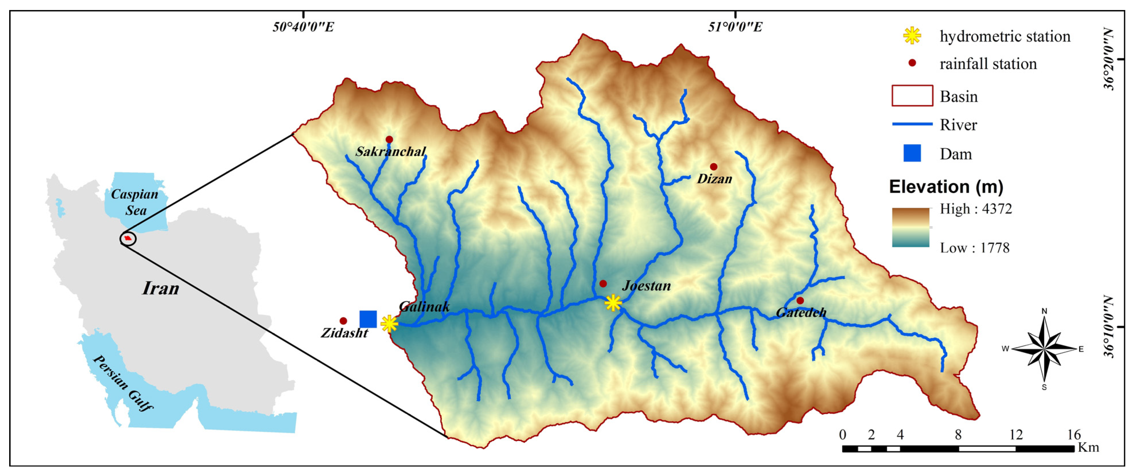
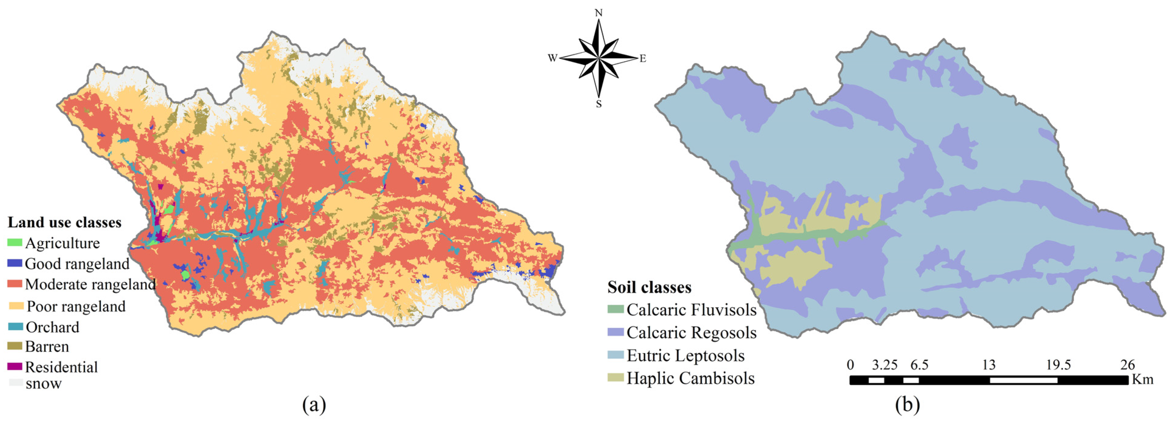
2.1. Description of the Study Area

The Taleghan watershed has an area of about 1325 km2, which comprises 2.3% of the Sefidrud Basin, Alborz province, Iran. The area under study is part of Taleghan watershed, covering an expanse of 805.58 km2. It lies upstream of the Taleghan dam, spanning latitudes from 36°5′ N to 35°21′ N and longitudes from 50°39′ E to 51°11′ E. This dam serves as a crucial source of drinking water required for Tehran province, Iran [49] (Figure 1). The watershed lies within a semi-arid region [48] and experiences a Mediterranean rainfall pattern, characterized by rainfall distribution throughout the year that aligns with the activity of wet systems in the west, northwest, and southwest regions. Notably, maximum rainfall occurs at the conclusion of the cold season, while minimal rainfall is observed during the hotter months, reflecting distinct seasonal patterns typical of the region. Temperature averages annually are 14.5 °C, with seasonal fluctuations ranging from a low of 1.3 °C in January to a peak of 26.3 °C in July. Based on data from the nearest climatological stations over a 20 year period, the watershed’s annual mean precipitation is recorded at 784.8 mm. Typically, approximately 70–80% of the mean annual rainfall in the study area occurs between November and May, predominantly in the form of snow [50]. The snowmelt season, occurring during spring (April, May, and June), accounts for the highest percentage of seasonal runoff, constituting 59% of the annual runoff. This significant contribution is not only attributed to rainfall but also to snowmelt, prompted by rising temperatures in the study area. Moreover, the months of May and June exhibit the highest monthly stream-flow percentages, representing 27% and 20% of the annual runoff, respectively [51]. The study area is characterized by its diverse topography, as the elevation within the watershed varies significantly, from 1778 m to 4374 m above sea level. The watershed’s average slope is steep, at 48%, and the Taleghan river overlength is 47.88 km by Galinak station. Predominantly, the watershed is covered by rangelands, which constitute about 84% of its land use. Additionally, it encompasses smaller areas of barren land, orchards, agricultural fields, and residential zones. The soil within the Taleghan watershed is primarily composed of silt loam and loam [50]. The location of the study area in Iran as well as the location of the stations used in this research are shown in Figure 1. In this research, the precipitation data of five rainfall stations and the runoff data of two hydrometric stations (Joestan and Galinak) were used. In addition, the meteorological data of Qazvin synoptic station (36°15′ N and 50°3′ E) were also used, which are not shown in the figure due to its distance from the study area. This station was the closest station to the study area.

2.2. Statistical DownScaling Model

The assessment of future climate change’s potential impact on hydrology was conducted through the application of downscaled climate projection outputs, utilizing the widely adopted SDSM [52]. SDSM facilitates the establishment of a statistical correlation between local-scale (predictand) and large-scale (predictors) climate variables during the downscaling process [17]. The necessary daily predictors for model calibration, including temperature, air pressure, geopotential height, and humidity, are sourced from reanalysis data obtained from the National Center for Environmental Prediction (NCEP), spanning the period from 1979 to 2014. The CanESM5 supplies future climate change scenarios from 2015 to 2100, which are instrumental in forecasting future climatic variables through SDSM. The selection of the most pertinent predictors, a critical aspect of the statistical downscaling process, is achieved by utilizing observed data to screen the predictors for specific predictands like precipitation, minimum, and maximum temperature within the study area [18]. This process is supported by an array of analytical tools including correlation matrices, partial correlations, p-values, histograms, and scatter plots to identify the most appropriate predictors. These predictors were sourced from the Canadian Climate Data and Scenarios database (http://climate-scenarios.canada.ca/ accessed on 30 November 2023), accessible at a spatial resolution of approximately 2.8°. In this study, SDSM version 4.2 was employed to downscale SSPs scenarios. The model underwent calibration and validation using available observational data spanning the years 1979–2000 and 2001–2012, respectively. Typically, a 30 year period is regarded as the baseline, as it provides sufficient time to capture local climate variations encompassing periods of drought, precipitation, temperature fluctuations, and other climatic phenomena [53]. Thus, the period from 1981 to 2011 was considered as the baseline period for this study. Climate change projections for rainfall and temperature were generated for the period from 2040 to 2070 under SSP126, SSP245, and SSP585. Furthermore, the performance of the baseline scenarios produced by SDSM models was evaluated using the Root Mean Square Error (RMSE), coefficient of determination (R2), and Nash–Sutcliffe Efficiency (NSE) metrics.

2.3. The Hydrological Model

To project water balance and runoff dynamics up to the year 2070, the SWAT is employed, incorporating the downscaled precipitation and temperature data from SDSM as inputs. Originally developed by the United States Department of Agriculture’s Agricultural Research Service [54], SWAT is a comprehensive, spatially distributed model that is both process- and physically based, operating in continuous time to simulate the quantity and quality of surface and subsurface water flows on a daily basis. It is adept at assessing the environmental consequences of various climate change scenarios, land use, and management practices on water resources [55]. The SWAT model utilizes the water balance equation to simulate the hydrological cycle.
For the GIS integration, ArcSWAT Version 2012.10 serves as an interface and extension within the ESRI ArcGIS Version 10.5.1 Desktop environment. ArcSWAT, a GIS-based graphical user interface available on the SWAT model’s website facilitates the delineation, subdivision, and parameterization of watersheds. It segments a watershed into sub-basins linked by a river network derived from a digital elevation model. Each sub-basin is further partitioned into hydrological response units (HRUs) characterized by distinct land use, soil, and slope profiles [55]. Initially, hydrological processes are modeled within each sub-basin, followed by the aggregation of simulated hydrological components toward the watershed’s outlet via the stream network, thereby enabling the simulation of various physical processes such as evapotranspiration, surface runoff, infiltration, lateral flow, and groundwater movement within the watershed study.

2.3.1. Model Setup

The Taleghan watershed was delineated into 63 sub-basins, further segmented into 875 HRUs within the SWAT model framework, based on a comprehensive analysis of the digital elevation model (DEM), land use patterns, and soil type distributions. The high-resolution DEM, with a granularity of 12.5 m × 12.5 m, was sourced from the Alaska Satellite Facility (http://search.asf.alaska.edu/accessed on 25 April 2020). Soil classifications were derived from a detailed survey conducted by the Tehran Regional Water Company, as documented in the soil survey report (Figure 2b) [56]. The land use/land cover (LULC) map was meticulously crafted using training points established from field surveys and Google Earth imagery, complemented by TM (https://earthexplorer.usgs.gov/ accessed on 9 April 2022) satellite imagery from 2020, and refined through the decision tree classification method (Figure 2a). It should be noted that the land use map remained constant throughout all periods analyzed in this study, and potential land use changes were not investigated.
Meteorological data, encompassing daily minimum and maximum temperatures, rainfall, relative humidity, solar radiation, and wind speed, were obtained from the Iran Meteorological Organization for the Qazvin station. Additionally, rainfall and hydrological datasets spanning from 2000 to 2018 were procured from the Basic Water Resources Studies Office of Tehran, Iran. The efficacy of the SWAT model in simulating runoff was meticulously evaluated at the Joestan and Galinak hydrological stations, with their precise locations depicted in Figure 1.
Despite continuous quality data evaluation and correction efforts by the Basic Water Resources Studies Office, initial preprocessing includes sorting the time series data, removing duplicate entries, rectifying apparent inaccuracies like decimal errors in data entry, and making necessary adjustment has been undertaken. These procedures are supported by the analysis of index plots and scatter plots.

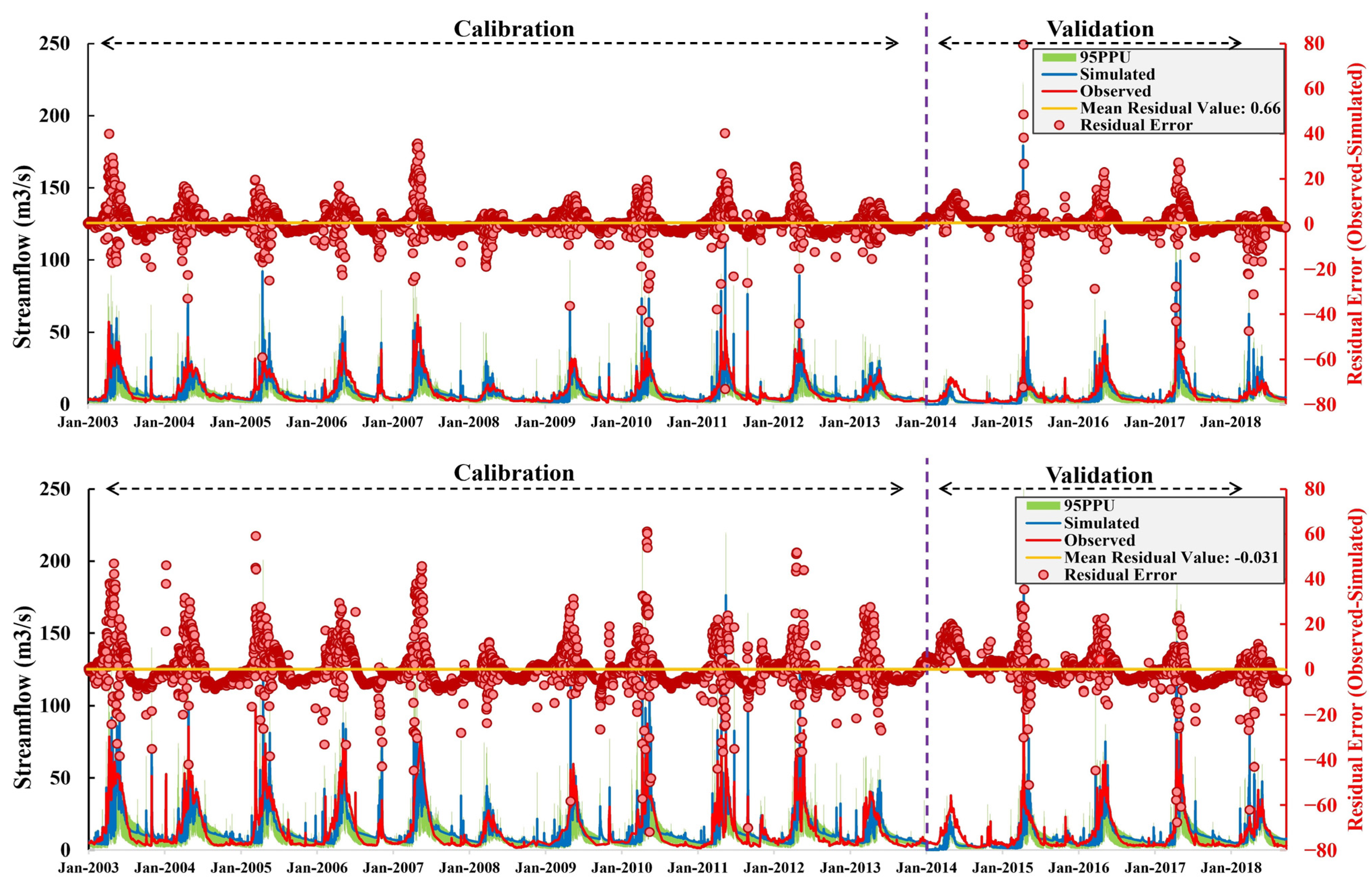
2.3.2. Model Evaluation

The model underwent calibration for the period 2003–2013, validation for 2014–2018, and a three-year warm-up phase from 2000 to 2002, with the former occupying three-fourths of the total period and the latter one-fourth. The selection of the validation period was predicated on the similarity of physical criteria, such as climate and land use, to those of the calibration period, ensuring consistency and reliability in model performance [57]. Both manual sensitivity analysis and automated calibration were used. The manual calibration of pivotal parameters for the quantification of hydrological components has unveiled profound insights into the catchment’s hydrologic behavior. Automated calibration facilitated by the SWAT-CUP program and the SUFI-2 algorithm [57,58,59] were employed to pinpoint and adjust critical parameters impacting runoff simulation.
Parameters that demonstrated significant sensitivity, particularly those related to snow processes, the Soil Conservation Service runoff curve number (CN2), and the baseflow alpha factor (days), are outlined in Table 1. In this study, priority was given to parameters exhibiting higher levels of uncertainty for model calibration. Consequently, parameters associated with soil characteristics were excluded from consideration, as the properties of the soil had been meticulously measured across 100 profiles, ensuring their accuracy.
Figure 3 presents a graphical depiction of the simulated discharge at the two scrutinized stations during both calibration and validation phases, demonstrating the model’s proficiency in capturing the general discharge. Although the residual error values indicate satisfactory model performance for the majority of the year, there are instances, particularly on days with higher discharge levels, where the error margin increases. One contributing factor to inaccuracies in semi-distributed models stems from input variables such as temperature and precipitation. These climatic data, collected at local meteorological stations, when regionalized, can lead to significant discrepancies, notably in areas with complex topography. Within the SWAT framework, climatic inputs for each subbasin are supplied by the meteorological station closest to the subbasin’s centroid. The challenge in precisely quantifying errors related to rainfall or temperature distribution arises from the necessity of data aggregation across numerous stations [60]. It is important to acknowledge that in this investigation, the introduction of five elevation bands aimed to mitigate such errors by refining temperature and precipitation adjustments to reflect the orographic influences within a subbasin.
The SWAT model’s efficacy was further scrutinized using the R2, NSE, and the percent bias (PBIAS), aligning with established evaluation metrics [57,61]. Table 2 summarizes the statistical results of the SWAT model’s efficacy at the Joestan and Galinak stations throughout the calibration (2003–2013) and validation (2014–2018) phases. The model’s capability in accurately simulating daily discharge at both stations was affirmed, with the NSE and R2 surpassing the 0.5 threshold, and the PBIAS remaining within the acceptable limit of 15% [62]. The model’s uncertainty was quantified through a 95% prediction uncertainty (95PPU) interval, established at the 2.5% and 97.5% confidence levels of the cumulative distribution, derived from parameter uncertainties propagated via Latin hypercube sampling. Model performance was adjudged satisfactory when the majority of observations fell within the 95PPU range. The model’s fit was quantitatively assessed using the P-factor and R-factor, where the P-factor indicates the percentage of observed data encapsulated within the 95PPU and values exceeding 70% were deemed acceptable. The R-factor, indicative of the 95PPU’s breadth, aimed for values below 1. Furthermore, the P-factor and R-factor metrics underscored the model’s satisfactory performance [60]. In general, model error can stem from parameter uncertainty, the measurement uncertainty of variables, and simplification error resulting from excessive model structure simplification [63]. Several uncertainties arise from anthropogenic influences, including the impact of wetlands and reservoirs on hydrological dynamics and significant infrastructural developments like roads, dams, tunnels, and bridges that can generate substantial sediment loads over several years, thereby altering water quantity and quality, as well as overlooked factors like fertilization, irrigation practices, water diversions, and various activities within river floodplains, such as farming and the disposal of construction debris [60]. The region examined in this study was largely unaffected by these human activities, thus confining model uncertainties primarily to errors stemming from simplified process representations and the measurement of variables.
Collectively, these results underscore the SWAT model’s robustness in daily streamflow simulation, especially at the Galinak station. One possible explanation for the model’s superior accuracy at the Galinak station compared to Joestan could be the higher quality of the measured rainfall and runoff data linked to the Galinak station. Furthermore, it is conceivable that the optimal values identified for sensitive parameters in the HRUs associated with the Galinak station better reflect real conditions.

2.4. Low Flow and High Flow

Projected daily streamflow values under SSP scenarios 126, 245, and 585 were analyzed to determine low and high flow event percentiles using the Flow Duration Curve (FDC). An FDC, which ranks flow data over a specific period by magnitude and delineates the percentage of time each flow level is exceeded [29], serves as a critical tool in hydrological assessments. It is particularly useful in water resource planning, such as the design of hydropower systems or water supply infrastructures, and in the evaluation of water quality [64]. For perennial streams, low flow threshold levels are typically identified between the 70th percentile flow (Q70, exceeded 70% of the time) and the 95th percentile flow (Q95) on the FDC [65]. This study adopts the 90th percentile exceedance frequency on the FDC to investigate extreme drought conditions, while the 5th percentile exceedance frequency is utilized to assess high flow events. These thresholds, Q5 and Q90, are recognized as standard indices in flow analysis [30,31,35].
Furthermore, the study employs annual maximum and minimum moving average discharges, metrics extensively used in delineating drought and flood phenomena [36,66,67]. High flow conditions are characterized by annual maximum discharges over 1 day, 3 day, and 7 day periods, derived from daily average discharge data. Conversely, low flow conditions are identified by annual minimum discharges over 7 day, 30 day, and 60 day periods, calculated from daily average discharge records at two hydrological stations. Focusing on annual flow minima, such as 7Q and 30Q, instead of continuous daily flow series helps reduce sensitivity to day-to-day fluctuations and artificial components of river flow. This approach makes the annual flow minima less vulnerable to measurement errors [68].

3. Results and Discussion

3.1. Evaluating the Performance of SDSM

The efficacy of the SDSM was rigorously evaluated using observational data from six terrestrial stations. Variables that exhibited a p-value (≤0.05) at a 95% confidence level were deemed suitable predictors. The most effective predictors identified for precipitation included P5_f (500 hPa air flow strength), P5_v (500 hPa meridional velocity), and prcp (precipitation), while temp (mean temperature at 2 m) was found to be the most effective for both minimum and maximum temperature during the calibration phase.
The performance of SDSM was further quantified using various statistical measures, including the RMSE, NSE, and R2 as summarized in Table 3. The analysis revealed that NSE and R values for precipitation and temperature ranged between 0.8 to 0.99 during both the calibration and validation periods, indicating satisfactory model performance [62]. Specifically, NSE values exceeding 0.5 are considered indicative of satisfactory model accuracy. The model exhibited commendable performance for precipitation and temperature data, aligning with findings from previous studies for precipitation [69] and temperature [70]. Comparing the ratio of RMSE to the observed average showed the higher accuracy of the model in temperature simulation, as evidenced by higher NSE and R2 values during both calibration and validation phases across all stations. However, the downscaling of precipitation data may be subject to various uncertainties, including the intricacies of local climate interactions, the coarse resolution of GCMs, their structural and parametric configurations, and the choice of downscaling techniques [71]. The examination of the model’s performance in downscaling precipitation across various stations revealed that the accuracy in different stations were similar.

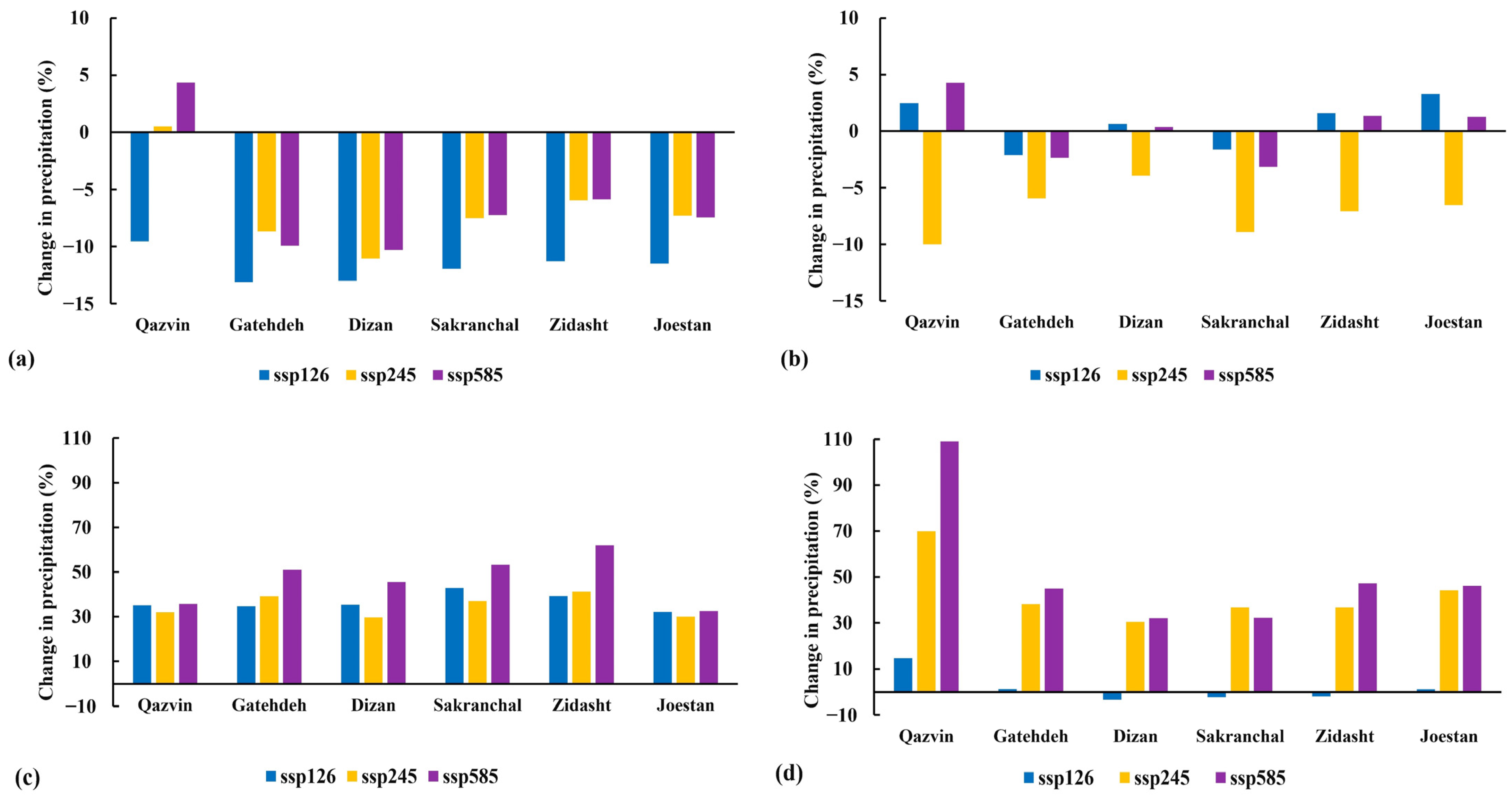
3.2. Projected Changes in Climate

In this study, the future climatic conditions, specifically maximum and minimum temperatures and precipitation levels for the period 2040–2070, were simulated under three SSP scenarios: SSP126, SSP245, and SSP585. The analysis revealed notable changes in monthly temperatures and seasonal precipitation patterns compared with historical records from 1981–2011, as illustrated in Figure 4 and Figure 5. February and March are projected to witness the most substantial increases in monthly average daily temperatures across all scenarios, as depicted in Figure 4. Relative to the reference period of 1981–2011, average daily maximum temperatures are expected to rise by 2.9 °C, 3.6 °C, and 5.1 °C under SSP126, SSP245, and SSP585 scenarios, respectively. Similarly, enhancements in average daily minimum temperatures are projected at 2.7 °C, 3.2 °C, and 4.6 °C across these scenarios, highlighting a pronounced warming trend particularly during the winter and early spring months. This trend indicates potential alterations in regional climate dynamics, with significant implications for hydrological processes.
Figure 5 presents the forecasted percentage changes in mean seasonal rainfall for the same future period in comparison to the historical baseline of 1981–2011, under the SSP scenarios. These data point to an increase in precipitation during the summer and autumn months, with the most significant rise observed in the autumn, where the increment varies from 14.6% to 109.2% across different scenarios. In contrast, a reduction in precipitation is anticipated during the winter months, with decreases ranging from 13% under SSP126 to 10% under SSP585. These projections suggest a future climate regime characterized by heightened temperatures and augmented rainfall, particularly in the later part of the year. The enhanced precipitation can be attributed to the increased capacity of warmer air to retain and subsequently release more water vapor, a phenomenon that underscores the likelihood of intensified hydrological cycles [72]. Consequently, these findings highlight the need for adaptive watershed management strategies to accommodate the expected changes in seasonal precipitation patterns and their ramifications for water resource allocation, agricultural activities, and environmental conservation.

3.3. Projected Changes in Hydrology

3.3.1. Variation in Hydrologic Variables under Future Climate Changes

The calibrated SWAT model was utilized to simulate hydrological responses under three future climate change scenarios (SSP126, SSP245, SSP585) for the period 2040–2070. Table 4 presents the simulated impacts on key hydrological variables such as mean annual precipitation, actual evapotranspiration, streamflow, lateral flow, snowfall, and snowmelt, highlighting potential changes due to climate variability for the case study. Notably, evapotranspiration is expected to surge by approximately 60% to 74% across the SSP scenarios, as a consequence of the anticipated temperature increases. In a study incorporating RCP4.5 and RCP8.5 scenarios, projections indicate an increase in precipitation and transpiration within this watershed during the period of 2020–2040 [73]. Lateral flow, or base flow, is also projected to rise under all scenarios, with the most significant changes expected under SSP585, followed by SSP245, indicating an overall increase in base flow ranging from 74% to 88% by 2070. This uptick in lateral flow is likely a result of increased precipitation and snowmelt. Conversely, surface runoff is anticipated to decline by 4% to 9.6%, attributed to elevated temperatures and enhanced evapotranspiration rates.
Based on the findings presented in Table 4, snowmelt has a significant impact on the water balance of the watershed. As there are no glaciers in the study area, any increase in snowmelt in the future will be a result of an increase in snowfall. Historically, snowfall began in December, followed by snowmelt in March, with the peak occurring in April. However, the assessment of the temporal snowmelt patterns outlined in Figure 6 suggests that snowmelt will begin earlier in the future period. As a result, the amount of snow melting is predicted to increase in February and March, while it is expected to decrease in April and May. This means that there will be less snow accumulation during the warmer months of the year and the reduction in snowfall and the melting of snow under the SSP585 aggravates this condition. In other research endeavors, it is extensively documented that future simulations often reveal an initial rise in wintertime discharge, succeeded by a decline in springtime discharge. This pattern is attributed to increasing temperatures, leading to earlier snowmelt and reduced snow accumulation [74,75].
Given the identical flow patterns observed in the Joestan and Galinak stations, the investigation focused on examining flow changes at the Galinak station situated at the watershed’s outlet. Figure 7 delineates the projected monthly discharge changes at two stations under the SSP scenarios. It is anticipated that discharge will rise under all scenarios, with more pronounced increases under SSP245 and SSP585, compared to SSP126. At the Galinak station, observations included discharge increases of 48% under SSP126, 53.6% under SSP245, and 52.6% under SSP585 by 2070. The figure illustrates a consistent forecast of increased runoff across all months, with a notable surge projected for February and March attributed to heightened snowmelt during this period. These projections underscore the potential impacts of climate change on discharge dynamics, which could exacerbate water management challenges, particularly during peak rainfall periods, affecting both water resource management and ecosystem health. This necessitates a reevaluation of existing infrastructure and adaptation strategies to accommodate the impending hydrological shifts.

3.3.2. Projected Change in Low Flow and High Flow

Figure 8 illustrates the FDC for Galinak station, providing a comparative analysis of hydrological regimes between the historical period (1981–2011) and the projected future period (2040–2070) under three SSP scenarios. This analysis reveals increases in both high and low flow conditions, particularly in low flow at this station. High flow events, occurring 5% of the time, are expected to surge, with an average increase of 20.6% under SSP245 and 17.2% under SSP585, while SSP585 forecasts a lesser yet substantial rise of about 9% by 2070. On the other hand, low flow conditions, represented by flows exceeding 90% of the time, are projected to experience a remarkable increase, ranging from 76% under SSP126 to 100% under SSP585, with SSP245 showing an intermediate increase of 88.6%.
In examining potential future hydrological drought conditions, annual minimum discharges over 7 day, 30 day, and 60 day periods were analyzed at two stations, with findings presented in Figure 9. The results indicate an overall increase in low flow due to heightened precipitation for the future period (2040–2070). Specifically, the annual 30 day minimum discharge is expected to rise by an average of 60% under SSP126, 71% under SSP245, and 80% under SSP585 compared to the historical baseline. The annual 60 day minimum discharge shows the greatest variability, with increases of 73% under SSP126, 94% under SSP245, and 115% under SSP585 by 2070.
Future flood scenarios were assessed by calculating annual maximum discharges for 1 day, 3 day, and 7 day periods with results depicted in Figure 10. The comparison between the annual average maximum flow for the future period and the base period revealed that the SSP585 scenario exhibits the highest variability, predicting a rise in annual maximum discharge by 44%, 25%, and 13% for 1 day, 3 day, and 7 day periods, respectively. Conversely, a decrease in 1 day maximum discharge by 14% and 10% is anticipated under SSP126 and SSP245, respectively, with a modest increase in 7 day maximum discharge by 7% and 6% under these scenarios. Although the changes in the maximum flow were less than the low flow, the examination of the maximum flow of 1 day duration for different years showed a sharp increase in the maximum flow for some years. The SSP585 scenario consistently indicates the most significant increase in high flow rates, suggesting that more severe climatic conditions yield more pronounced hydrological effects. The SSP126 and SSP245 scenarios also project increases, albeit to a lesser extent, highlighting the differential impacts of various climate scenarios on hydrological extremes.
Under conditions of climate change, total water resources are anticipated to rise due to an increase in precipitation, with both low flow and high flow set to escalate across all three scenarios. Per the FDC analysis, the SSP585 scenario exhibited the smallest increase in high flow rates. Yet, when evaluating maximum flows over different durations (e.g., 1 day, 3 day, and 7 day maximum flows), the highest flow values were recorded under SSP585. This implies that, under pessimistic projections, high flow rates have markedly risen in certain years. According to these results, more severe hydrological conditions are expected.

4. Conclusions

This investigation delineates the dynamics of the hydrological equilibrium and the extremities of flow patterns within a semi-arid Mediterranean basin located in Iran, employing a meticulous examination of future climatic projections derived from the CanESM5 model, across three distinct SSP scenarios (ssp126, ssp245, ssp585). The salient findings are as follows:
  • The advent of climate change portends an upsurge in both precipitation and temperature across all SSP projections. Between 2040 and 2070, the anticipated modifications in the average diurnal maximum and minimum temperatures are projected at 2.9 °C, 3.6 °C, and 5.1 °C, alongside 2.7 °C, 3.2 °C, and 4.6 °C under SSP126, SSP245, and SSP585, respectively, compared to the historical period 1981 to 2011. Precipitation is foreseen to experience shifts of 52.6%, 58.8%, and 60%. An analysis of seasonal precipitation trends indicates an escalation in rainfall during the summer and autumn, contrasted with a reduction in the winter season.
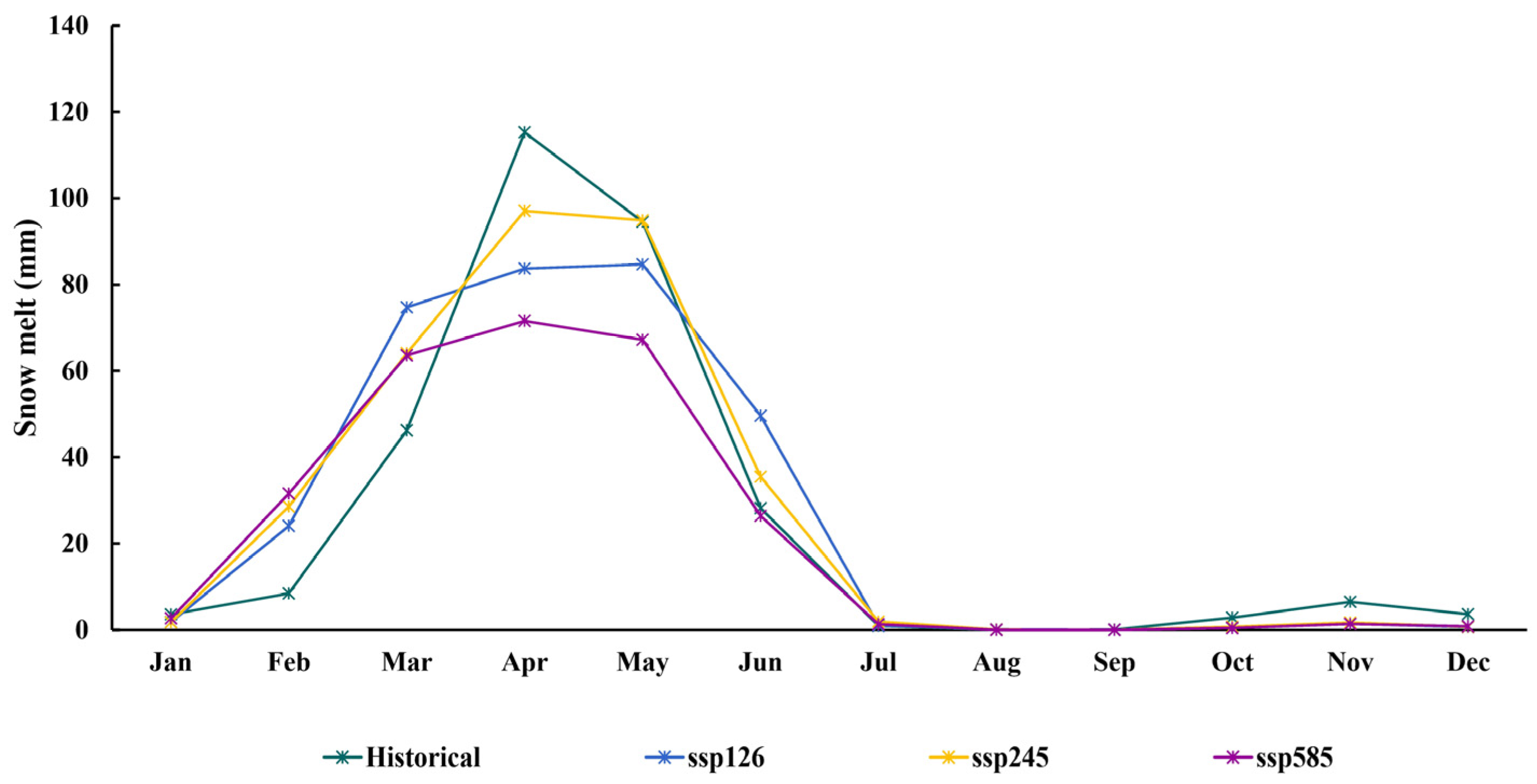
  • Relative to historical records, pronounced deviations are noted across essential hydrological constituents. Evapotranspiration has registered changes between 60.5% and 74%, while surface runoff has varied from −4.1% to −9.6%, and snowmelt projections indicate a 15% and 15.7% increase under SSP126 and SSP245, respectively, with a −4.2% decrease under SSP585. The analysis of the changes in the timing of snow melting revealed a shift correlated with rising temperatures. Specifically, the onset of snow melting increased from March to February, while the quantity of snow melting in April (typically the peak period) decreased. These outcomes underscore substantial shifts in hydrological functions, accentuating the ramifications of climatic alterations on the Taleghan watershed’s hydrological balance.
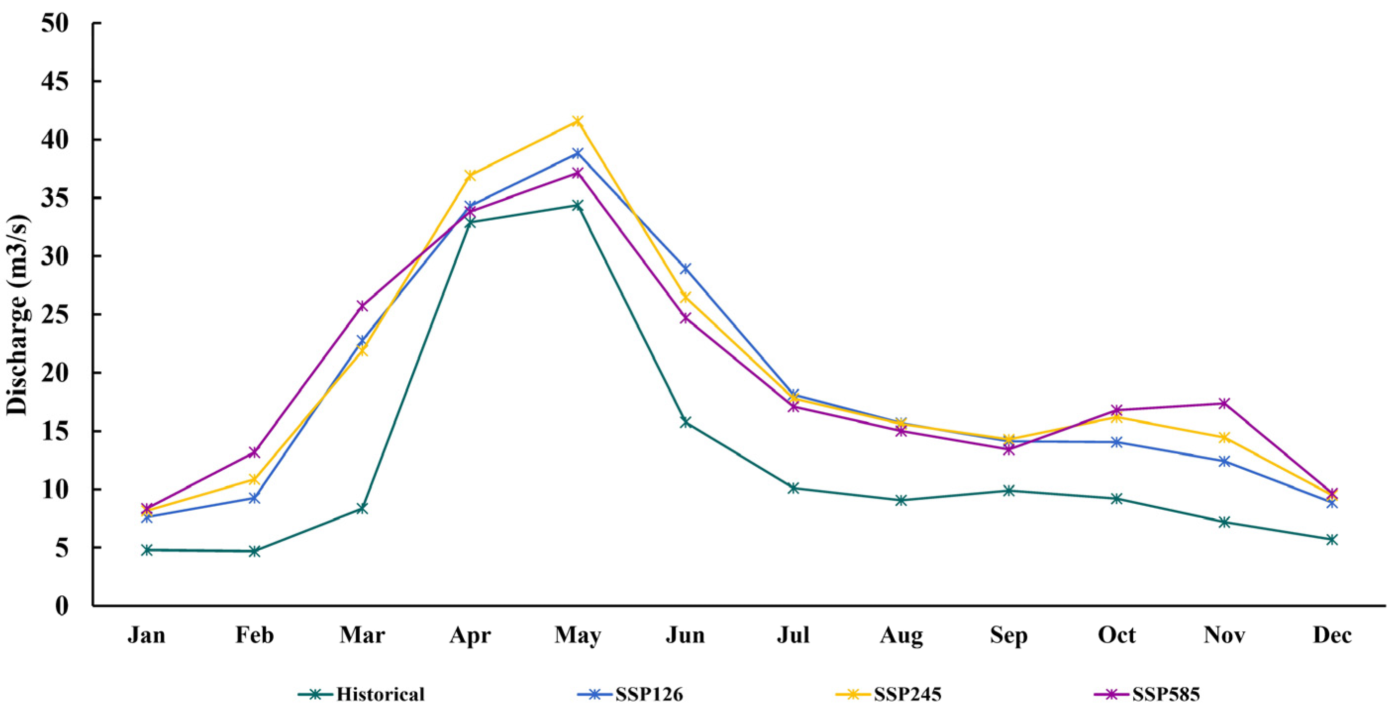
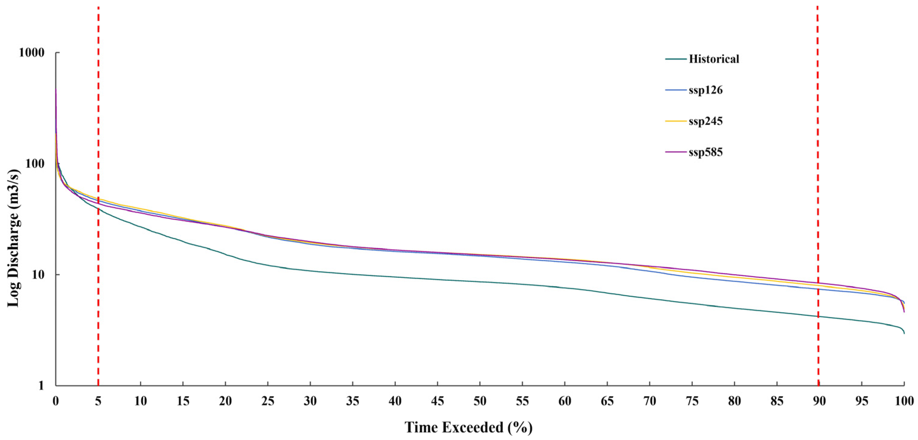
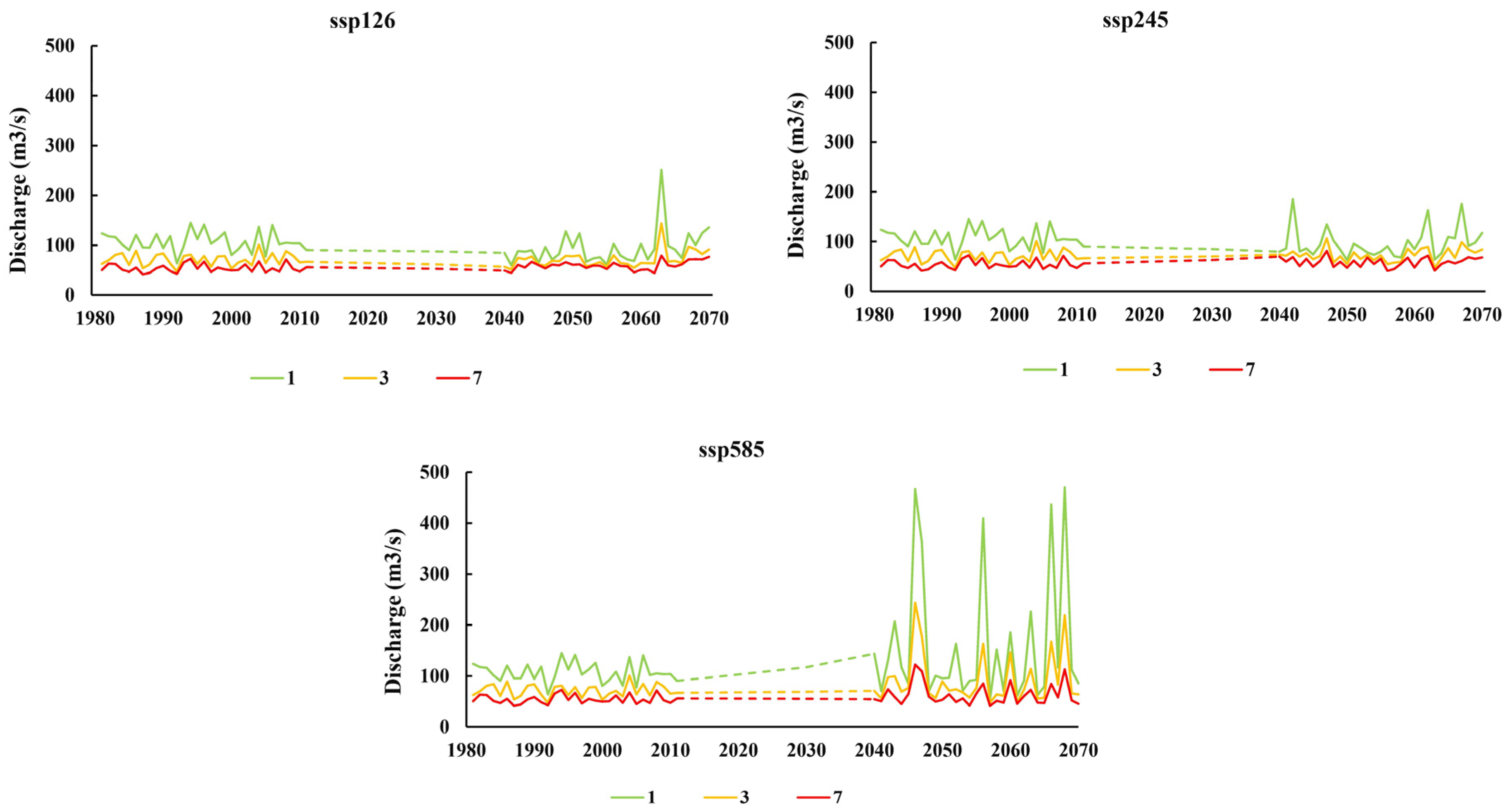
  • Within the Taleghan basin, climate scenarios forecasted increased alterations in evapotranspiration, lateral flow, snowmelt, discharge, low and high flows, whereas surface runoff exhibited a negative trajectory.
The results underscore the necessity for heightened awareness regarding the potential future consequences of climatic fluctuations on both water balance and flood risks within this river basin. Consequently, policymakers in the catchment area must prioritize the formulation of climate adaptation strategies, emphasizing flood control, evapotranspiration reduction, and water resource conservation. These measures are essential for bolstering environmental and economic resilience in the face of changing climate patterns. Future research endeavors should venture into the exploration of uncertainties inherent within various large-scale models and divergent downscaling methodologies. The integration of analyses to gauge the impact of land cover/use modifications attributable to climatic variations is recommended. Augmenting the repertoire of hydrological models beyond the confines of SWAT is advocated to refine the precision of insights into hydrological responses amid climate change.

Author Contributions

Conceptualization, M.H.M. and A.N.S.; methodology, M.H.M., A.N.S. and A.Z.G.; software, M.H.M.; validation, A.N.S., A.Z.G. and M.M.R.; formal analysis, V.S.; investigation, M.H.M. and V.S.; resources, M.M.R.; data curation, A.N.S. and A.Z.G.; writing—original draft preparation, M.H.M. and V.S.; writing—review and editing, V.S. and M.M.R.; visualization, V.S.; supervision, A.N.S. and M.M.R. All authors have read and agreed to the published version of the manuscript.

Funding

This research received no external funding.

Data Availability Statement

The data presented in this study are available upon corroborated re-quest from the corresponding author. The meteorological data used in this study are confidential and not publicly available.

Acknowledgments

The authors would like to thank the Meteorological Organization and Regional Water Company of Tehran, Iran for providing the data used in this study.

Conflicts of Interest

The authors declare no conflicts of interest.

References

  1. Trenberth, K. Changes in Precipitation with Climate Change. Clim. Res. 2011, 47, 123–138. [Google Scholar] [CrossRef]
  2. Lavers, D.A.; Ralph, F.M.; Waliser, D.E.; Gershunov, A.; Dettinger, M.D. Climate Change Intensification of Horizontal Water Vapor Transport in CMIP5. Geophys. Res. Lett. 2015, 42, 5617–5625. [Google Scholar] [CrossRef]
  3. Wang, L.; Shu, Z.; Wang, G.; Sun, Z.; Yan, H.; Bao, Z. Analysis of Future Meteorological Drought Changes in the Yellow River Basin under Climate Change. Water 2022, 14, 1896. [Google Scholar] [CrossRef]
  4. Huntington, T.G. Evidence for Intensification of the Global Water Cycle: Review and Synthesis. J. Hydrol. 2006, 319, 83–95. [Google Scholar] [CrossRef]
  5. Guyasa, A.K.; Guan, Y.; Zhang, D. Impact of Climate Change on the Water Balance of the Akaki Catchment. Water 2023, 16, 54. [Google Scholar] [CrossRef]
  6. Jung, I.W.; Bae, D.H.; Lee, B.J. Possible Change in Korean Streamflow Seasonality Based on Multi-model Climate Projections. Hydrol. Process. 2013, 27, 1033–1045. [Google Scholar] [CrossRef]
  7. Nie, T.; Yuan, R.; Liao, S.; Zhang, Z.; Gong, Z.; Zhao, X.; Chen, P.; Li, T.; Lin, Y.; Du, C.; et al. Characteristics of Potential Evapotranspiration Changes and Its Climatic Causes in Heilongjiang Province from 1960 to 2019. Agriculture 2022, 12, 2017. [Google Scholar] [CrossRef]
  8. Stone, M.C.; Hotchkiss, R.H.; Hubbard, C.M.; Fontaine, T.A.; Mearns, L.O.; Arnold, J.G. Impacts of Climate Change on Missouri Rwer Basin Water Yield 1. J. Am. Water Resour. Assoc. 2001, 37, 1119–1129. [Google Scholar] [CrossRef]
  9. Intergovernmental Panel on Climate Change (IPCC). Climate Change 2022—Impacts, Adaptation and Vulnerability; Cambridge University Press: Cambridge, UK, 2022; ISBN 9781009325844. [Google Scholar]
  10. Ghafouri-Azar, M.; Kim, J.; Bae, D. Assessment of the Potential Changes in Low Flow Projections Estimated by Coupled Model Intercomparison Project Phase 5 Climate Models at Monthly and Seasonal Scales. Int. J. Climatol. 2021, 41, 3222–3236. [Google Scholar] [CrossRef]
  11. Meehl, G.A.; Senior, C.A.; Eyring, V.; Flato, G.; Lamarque, J.-F.; Stouffer, R.J.; Taylor, K.E.; Schlund, M. Context for Interpreting Equilibrium Climate Sensitivity and Transient Climate Response from the CMIP6 Earth System Models. Sci. Adv. 2020, 6, eaba1981. [Google Scholar] [CrossRef]
  12. O’Neill, B.C.; Carter, T.R.; Ebi, K.; Harrison, P.A.; Kemp-Benedict, E.; Kok, K.; Kriegler, E.; Preston, B.L.; Riahi, K.; Sillmann, J.; et al. Achievements and Needs for the Climate Change Scenario Framework. Nat. Clim. Chang. 2020, 10, 1074–1084. [Google Scholar] [CrossRef]
  13. Peng, S.; Wang, C.; Li, Z.; Mihara, K.; Kuramochi, K.; Toma, Y.; Hatano, R. Climate Change Multi-Model Projections in CMIP6 Scenarios in Central Hokkaido, Japan. Sci. Rep. 2023, 13, 230. [Google Scholar] [CrossRef]
  14. Eekhout, J.P.C.; de Vente, J. Global Impact of Climate Change on Soil Erosion and Potential for Adaptation through Soil Conservation. Earth-Sci. Rev. 2022, 226, 103921. [Google Scholar] [CrossRef]
  15. Boé, J.; Terray, L.; Habets, F.; Martin, E. Statistical and Dynamical Downscaling of the Seine Basin Climate for Hydro-meteorological Studies. Int. J. Climatol. 2007, 27, 1643–1655. [Google Scholar] [CrossRef]
  16. Gebrechorkos, S.H.; Bernhofer, C.; Hülsmann, S. Climate Change Impact Assessment on the Hydrology of a Large River Basin in Ethiopia Using a Local-Scale Climate Modelling Approach. Sci. Total Environ. 2020, 742, 140504. [Google Scholar] [CrossRef] [PubMed]
  17. Wilby, R.L.; Dawson, C.W. The Statistical DownScaling Model: Insights from One Decade of Application. Int. J. Climatol. 2013, 33, 1707–1719. [Google Scholar] [CrossRef]
  18. Peng, S.; Wang, C.; Eguchi, S.; Kuramochi, K.; Kohyama, K.; Yoshikawa, S.; Itahashi, S.; Igura, M.; Ohkoshi, S.; Hatano, R. Response of Hydrological Processes to Climate and Land Use Changes in Hiso River Watershed, Fukushima, Japan. Phys. Chem. Earth Parts A/B/C 2021, 123, 103010. [Google Scholar] [CrossRef]
  19. Getachew, B.; Manjunatha, B.R.; Bhat, H.G. Modeling Projected Impacts of Climate and Land Use/Land Cover Changes on Hydrological Responses in the Lake Tana Basin, Upper Blue Nile River Basin, Ethiopia. J. Hydrol. 2021, 595, 125974. [Google Scholar] [CrossRef]
  20. Eingrüber, N.; Korres, W. Climate Change Simulation and Trend Analysis of Extreme Precipitation and Floods in the Mesoscale Rur Catchment in Western Germany until 2099 Using Statistical Downscaling Model (SDSM) and the Soil & Water Assessment Tool (SWAT Model). Sci. Total Environ. 2022, 838, 155775. [Google Scholar] [CrossRef] [PubMed]
  21. Wang, Q.; Xu, Y.; Wang, Y.; Zhang, Y.; Xiang, J.; Xu, Y.; Wang, J. Individual and Combined Impacts of Future Land-Use and Climate Conditions on Extreme Hydrological Events in a Representative Basin of the Yangtze River Delta, China. Atmos. Res. 2020, 236, 104805. [Google Scholar] [CrossRef]
  22. Gebrechorkos, S.H.; Bernhofer, C.; Hülsmann, S. Impacts of Projected Change in Climate on Water Balance in Basins of East Africa. Sci. Total Environ. 2019, 682, 160–170. [Google Scholar] [CrossRef]
  23. Worku, M.A.; Feyisa, G.L.; Beketie, K.T.; Garbolino, E. Projecting Future Precipitation Change across the Semi-Arid Borana Lowland, Southern Ethiopia. J. Arid Land 2023, 15, 1023–1036. [Google Scholar] [CrossRef]
  24. Goodarzi, M.R.; Abedi, M.J.; Heydari Pour, M. Climate Change and Trend Analysis of Precipitation and Temperature: A Case Study of Gilan, Iran. In Current Directions in Water Scarcity Research; Elsevier: Amsterdam, The Netherlands, 2022; pp. 561–587. [Google Scholar]
  25. Naderi, M.; Saatsaz, M.; Behrouj Peely, A. Extreme Climate Events under Global Warming in Iran. Hydrol. Sci. J. 2024. accepted. [Google Scholar] [CrossRef]
  26. Zarrin, A.; Dadashi-Roudbari, A. Evaluation of CMIP6 Models in Estimating Temperature in Iran with Emphasis on Equilibrium Climate Sensitivity (ECS) and Transient Climate Response (TCR). Iran. J. Geophys. 2023, 17, 39–56. (In Persian) [Google Scholar]
  27. Vetter, T.; Reinhardt, J.; Flörke, M.; van Griensven, A.; Hattermann, F.; Huang, S.; Koch, H.; Pechlivanidis, I.G.; Plötner, S.; Seidou, O.; et al. Evaluation of Sources of Uncertainty in Projected Hydrological Changes under Climate Change in 12 Large-Scale River Basins. Clim. Chang. 2017, 141, 419–433. [Google Scholar] [CrossRef]
  28. Stefanidis, K.; Panagopoulos, Y.; Mimikou, M. Response of a Multi-Stressed Mediterranean River to Future Climate and Socio-Economic Scenarios. Sci. Total Environ. 2018, 627, 756–769. [Google Scholar] [CrossRef] [PubMed]
  29. Ghafouri-Azar, M.; Bae, D.-H. Analyzing the Variability in Low-Flow Projections under GCM CMIP5 Scenarios. Water Resour. Manag. 2019, 33, 5035–5050. [Google Scholar] [CrossRef]
  30. Yan, D.; Werners, S.E.; Ludwig, F.; Huang, H.Q. Hydrological Response to Climate Change: The Pearl River, China under Different RCP Scenarios. J. Hydrol. Reg. Stud. 2015, 4, 228–245. [Google Scholar] [CrossRef]
  31. Huang, S.; Krysanova, V.; Hattermann, F.F. Projection of Low Flow Conditions in Germany under Climate Change by Combining Three RCMs and a Regional Hydrological Model. Acta Geophys. 2013, 61, 151–193. [Google Scholar] [CrossRef]
  32. Reddy, N.M.; Saravanan, S.; Almohamad, H.; Al Dughairi, A.A.; Abdo, H.G. Effects of Climate Change on Streamflow in the Godavari Basin Simulated Using a Conceptual Model Including CMIP6 Dataset. Water 2023, 15, 1701. [Google Scholar] [CrossRef]
  33. Meresa, H.; Donegan, S.; Golian, S.; Murphy, C. Simulated Changes in Seasonal and Low Flows with Climate Change for Irish Catchments. Water 2022, 14, 1556. [Google Scholar] [CrossRef]
  34. Lane, R.A.; Kay, A.L. Climate Change Impact on the Magnitude and Timing of Hydrological Extremes Across Great Britain. Front. Water 2021, 3, 684982. [Google Scholar] [CrossRef]
  35. Whitehead, P.G.; Barbour, E.; Futter, M.N.; Sarkar, S.; Rodda, H.; Caesar, J.; Butterfield, D.; Jin, L.; Sinha, R.; Nicholls, R.; et al. Impacts of Climate Change and Socio-Economic Scenarios on Flow and Water Quality of the Ganges, Brahmaputra and Meghna (GBM) River Systems: Low Flow and Flood Statistics. Environ. Sci. Process. Impacts 2015, 17, 1057–1069. [Google Scholar] [CrossRef] [PubMed]
  36. Yang, S.; Yang, D.; Zhao, B.; Ma, T.; Lu, W.; Santisirisomboon, J. Future Changes in High and Low Flows under the Impacts of Climate and Land Use Changes in the Jiulong River Basin of Southeast China. Atmosphere 2022, 13, 150. [Google Scholar] [CrossRef]
  37. Ghermezcheshmeh, B.; Goodarzi, M.; Hajimohammadi, M. Simulation of Low Flow Using SWAT under Climate Change Status. Water Harvest. Res. 2021, 4, 191–209. [Google Scholar] [CrossRef]
  38. Costigan, K.H.; Kennard, M.J.; Leigh, C.; Sauquet, E.; Datry, T.; Boulton, A.J. Flow Regimes in Intermittent Rivers and Ephemeral Streams. In Intermittent Rivers and Ephemeral Streams; Elsevier: Amsterdam, The Netherlands, 2017; pp. 51–78. [Google Scholar]
  39. Sauquet, E.; Shanafield, M.; Hammond, J.C.; Sefton, C.; Leigh, C.; Datry, T. Classification and Trends in Intermittent River Flow Regimes in Australia, Northwestern Europe and USA: A Global Perspective. J. Hydrol. 2021, 597, 126170. [Google Scholar] [CrossRef]
  40. Oueslati, O.; De Girolamo, A.M.; Abouabdillah, A.; Kjeldsen, T.R.; Lo Porto, A. Classifying the Flow Regimes of Mediterranean Streams Using Multivariate Analysis. Hydrol. Process. 2015, 29, 4666–4682. [Google Scholar] [CrossRef]
  41. Tramblay, Y.; Rutkowska, A.; Sauquet, E.; Sefton, C.; Laaha, G.; Osuch, M.; Albuquerque, T.; Alves, M.H.; Banasik, K.; Beaufort, A.; et al. Trends in Flow Intermittence for European Rivers. Hydrol. Sci. J. 2021, 66, 37–49. [Google Scholar] [CrossRef]
  42. Gutiérrez-Jurado, K.Y.; Partington, D.; Batelaan, O.; Cook, P.; Shanafield, M. What Triggers Streamflow for Intermittent Rivers and Ephemeral Streams in Low-Gradient Catchments in Mediterranean Climates. Water Resour. Res. 2019, 55, 9926–9946. [Google Scholar] [CrossRef]
  43. Alizadeh-Choobari, O.; Najafi, M.S. Extreme Weather Events in Iran under a Changing Climate. Clim. Dyn. 2018, 50, 249–260. [Google Scholar] [CrossRef]
  44. Mousavi, R.; Ahmadizadeh, M.; Marofi, S. A Multi-GCM Assessment of the Climate Change Impact on the Hydrology and Hydropower Potential of a Semi-Arid Basin (A Case Study of the Dez Dam Basin, Iran). Water 2018, 10, 1458. [Google Scholar] [CrossRef]
  45. Azari, M.; Moradi, H.R.; Saghafian, B.; Faramarzi, M. Climate Change Impacts on Streamflow and Sediment Yield in the North of Iran. Hydrol. Sci. J. 2016, 61, 123–133. [Google Scholar] [CrossRef]
  46. Maghsood, F.F.; Moradi, H.; Massah Bavani, A.R.; Panahi, M.; Berndtsson, R.; Hashemi, H. Climate Change Impact on Flood Frequency and Source Area in Northern Iran under CMIP5 Scenarios. Water 2019, 11, 273. [Google Scholar] [CrossRef]
  47. Tabari, H.; Abghari, H.; Hosseinzadeh Talaee, P. Temporal Trends and Spatial Characteristics of Drought and Rainfall in Arid and Semiarid Regions of Iran. Hydrol. Process. 2012, 26, 3351–3361. [Google Scholar] [CrossRef]
  48. Dodangeh, E.; Shahedi, K.; Solaimani, K.; Kossieris, P. Usability of the BLRP Model for Hydrological Applications in Arid and Semi-Arid Regions with Limited Precipitation Data. Model. Earth Syst. Environ. 2017, 3, 539–555. [Google Scholar] [CrossRef]
  49. Noor, H.; Vafakhah, M.; Mohammady, M. Comparison of Different Targeting Methods for Watershed Management Practices Implementation in Taleghan Dam Watershed, Iran. Water Supply 2016, 16, 1484–1496. [Google Scholar] [CrossRef]
  50. Faculty of Agriculture, University of Tehran (FAUT). General Investigation of Taleghan Basin: Hydrometeorology and Climatology Report; Regional Water Company of Tehran: Tehran, Iran, 1993. (In Persian) [Google Scholar]
  51. Vafakhah, M.; Nouri, A.; Alavipanah, S.K. Snowmelt-Runoff Estimation Using Radiation SRM Model in Taleghan Watershed. Environ. Earth Sci. 2015, 73, 993–1003. [Google Scholar] [CrossRef]
  52. Wilby, R.; Dawson, C.; Barrow, E. Sdsm—A Decision Support Tool for the Assessment of Regional Climate Change Impacts. Environ. Model. Softw. 2002, 17, 145–157. [Google Scholar] [CrossRef]
  53. Gebremeskel, S.; Liu, Y.B.; de Smedt, F.; Hoffmann, L.; Pfister, L. Analysing the Effect of Climate Changes on Streamflow Using Statistically Downscaled GCM Scenarios. Int. J. River Basin Manag. 2004, 2, 271–280. [Google Scholar] [CrossRef]
  54. Arnold, J.G.; Srinivasan, R.; Muttiah, R.S.; Williams, J.R. Large Area Hydrologic Modeling and Assessment PART I: Model Development. J. Am. Water Resour. Assoc. 1998, 34, 73–89. [Google Scholar] [CrossRef]
  55. Neitsch, S.L.; Arnold, J.; Kiniry, J.R.; Williams, J. Soil and Water Assessment Tool Theoretical Documentation Version 2009; Texas Water Resources Institute: College Station, TX, USA, 2011. [Google Scholar]
  56. Refahi, H.; Sarmadian, F. General Investigation of Taleghan Basin: Assessment of Land Resources and Capabilities Report; Regional Water Company of Tehran: Tehran, Iran, 1993. (In Persian) [Google Scholar]
  57. Abbaspour, K.; Vaghefi, S.; Srinivasan, R. A Guideline for Successful Calibration and Uncertainty Analysis for Soil and Water Assessment: A Review of Papers from the 2016 International SWAT Conference. Water 2017, 10, 6. [Google Scholar] [CrossRef]
  58. Badora, D.; Wawer, R.; Król-Badziak, A.; Nieróbca, A.; Kozyra, J.; Jurga, B. Hydrological Balance in the Vistula Catchment under Future Climates. Water 2023, 15, 4168. [Google Scholar] [CrossRef]
  59. Zewde, N.T.; Denboba, M.A.; Tadesse, S.A.; Getahun, Y.S. Predicting Runoff and Sediment Yields Using Soil and Water Assessment Tool (SWAT) Model in the Jemma Subbasin of Upper Blue Nile, Central Ethiopia. Environ. Chall. 2024, 14, 100806. [Google Scholar] [CrossRef]
  60. Abbaspour, K.C.; Yang, J.; Maximov, I.; Siber, R.; Bogner, K.; Mieleitner, J.; Zobrist, J.; Srinivasan, R. Modelling Hydrology and Water Quality in the Pre-Alpine/Alpine Thur Watershed Using SWAT. J. Hydrol. 2007, 333, 413–430. [Google Scholar] [CrossRef]
  61. Mengistu, T.D.; Chung, I.-M.; Kim, M.-G.; Chang, S.W.; Lee, J.E. Impacts and Implications of Land Use Land Cover Dynamics on Groundwater Recharge and Surface Runoff in East African Watershed. Water 2022, 14, 2068. [Google Scholar] [CrossRef]
  62. Moriasi, D.N.; Arnold, J.G.; Van Liew, M.W.; Bingner, R.L.; Harmel, R.D.; Veith, T.L. Model Evaluation Guidelines for Systematic Quantification of Accuracy in Watershed Simulations. Trans. ASABE 2007, 50, 885–900. [Google Scholar] [CrossRef]
  63. Cao, W.; Bowden, W.B.; Davie, T.; Fenemor, A. Multi-Variable and Multi-Site Calibration and Validation of SWAT in a Large Mountainous Catchment with High Spatial Variability. Hydrol. Process. 2006, 20, 1057–1073. [Google Scholar] [CrossRef]
  64. Croker, K.M.; Young, A.R.; Zaidman, M.D.; Rees, H.G. Flow Duration Curve Estimation in Ephemeral Catchments in Portugal. Hydrol. Sci. J. 2003, 48, 427–439. [Google Scholar] [CrossRef]
  65. Fleig, A.K.; Tallaksen, L.M.; Hisdal, H.; Demuth, S. A Global Evaluation of Streamflow Drought Characteristics. Hydrol. Earth Syst. Sci. 2006, 10, 535–552. [Google Scholar] [CrossRef]
  66. Lee, M.; Qiu, L.; Ha, S.; Im, E.; Bae, D. Future Projection of Low Flows in the Chungju Basin, Korea and Their Uncertainty Decomposition. Int. J. Climatol. 2022, 42, 157–174. [Google Scholar] [CrossRef]
  67. Naz, B.S.; Kao, S.-C.; Ashfaq, M.; Gao, H.; Rastogi, D.; Gangrade, S. Effects of Climate Change on Streamflow Extremes and Implications for Reservoir Inflow in the United States. J. Hydrol. 2018, 556, 359–370. [Google Scholar] [CrossRef]
  68. Smakhtin, V. Low Flow Hydrology: A Review. J. Hydrol. 2001, 240, 147–186. [Google Scholar] [CrossRef]
  69. Akhter, M.S.; Shamseldin, A.Y.; Melville, B.W. Comparison of Dynamical and Statistical Rainfall Downscaling of CMIP5 Ensembles at a Small Urban Catchment Scale. Stoch. Environ. Res. Risk Assess. 2019, 33, 989–1012. [Google Scholar] [CrossRef]
  70. Hasan, D.S.N.A.P.A.; Ratnayake, U.; Shams, S.; Nayan, Z.B.H.; Rahman, E.K.A. Prediction of Climate Change in Brunei Darussalam Using Statistical Downscaling Model. Theor. Appl. Climatol. 2018, 133, 343–360. [Google Scholar] [CrossRef]
  71. Chim, K.; Tunnicliffe, J.; Shamseldin, A.; Chan, K. Identifying Future Climate Change and Drought Detection Using CanESM2 in the Upper Siem Reap River, Cambodia. Dyn. Atmos. Ocean. 2021, 94, 101182. [Google Scholar] [CrossRef]
  72. Sadiqi, S.S.J.; Nam, W.-H.; Lim, K.-J.; Hong, E. Investigating Nonpoint Source and Pollutant Reduction Effects under Future Climate Scenarios: A SWAT-Based Study in a Highland Agricultural Watershed in Korea. Water 2024, 16, 179. [Google Scholar] [CrossRef]
  73. Tayebzadeh Moghadam, N.; Abbaspour, K.C.; Malekmohammadi, B.; Schirmer, M.; Yavari, A.R. Spatiotemporal Modelling of Water Balance Components in Response to Climate and Landuse Changes in a Heterogeneous Mountainous Catchment. Water Resour. Manag. 2021, 35, 793–810. [Google Scholar] [CrossRef]
  74. Zhou, Y.; Xu, Y.; Xiao, W.; Wang, J.; Huang, Y.; Yang, H. Climate Change Impacts on Flow and Suspended Sediment Yield in Headwaters of High-Latitude Regions—A Case Study in China’s Far Northeast. Water 2017, 9, 966. [Google Scholar] [CrossRef]
  75. Fang, G.; Yang, J.; Chen, Y.; Li, Z.; De Maeyer, P. Impact of GCM Structure Uncertainty on Hydrological Processes in an Arid Area of China. Hydrol. Res. 2018, 49, 893–907. [Google Scholar] [CrossRef]
Figure 1. The location of the study area in Iran, rainfall and hydrometric stations and stream network.
Water 16 00805 g001
Figure 2. Land use classes (a) and soil classes (b) of the study area.
Water 16 00805 g002
Figure 3. Calibration and validation results of observed vs. simulated daily streamflow at Joestan and Galinak stations. The calibration period spanned 2003–2013, while 2014–2018 served as the validation period.
Water 16 00805 g003
Figure 4. Projected changes in maximum (a) and minimum (b) temperatures (°C) for the period 2040–2070 under SSP126, SSP245, and SSP585.
Water 16 00805 g004
Figure 5. Percentage change in seasonal mean precipitation for the future period 2040–2070 under SSP126, SSP245, and SSP585, compared to the historical period 1981–2011: (a) winter, (b) spring, (c) summer, (d) fall.
Water 16 00805 g005
Figure 6. Monthly snowmelt comparison between current (1981–2011) and future (2040–2070) under SSP126, SSP245, and SSP585.
Water 16 00805 g006
Figure 7. Monthly runoff comparison between current (1981–2011) and future (2040–2070) under SSP126, SSP245, and SSP585 at Galinak station.
Water 16 00805 g007
Figure 8. Flow duration curve comparing Q5 (the left red dotted line) and Q90 (the right red dotted line) for current (1981–2011) and future (2040–2070) conditions under SSP126, SSP245, and SSP585 at Galinak station.
Water 16 00805 g008
Figure 9. Projected annual 7 day, 30 day, and 60 day minimum discharge under SSP126, SSP245, and SSP585, Galinak station.
Water 16 00805 g009
Figure 10. Projected annual 1 day, 3 day, and 7 day maximum discharge under SSP126, SSP245, and SSP585 Galinak station.
Water 16 00805 g010
Table 1. Calibration of Sensitive Parameters in the SWAT Model.
ParameterMin. ValueMax. ValueFitted Value
Maximum snow melting rate during the summer solstice.03.52.4
Snowfall temperature12.52.46
Initial SCS curve number II−0.050.05−0.03
Soil evaporation adjustment factor00.950.76
Threshold depth for return flow (mm)070038.5
Baseflow alpha (days)00.0130.005
Snow melt temperature031.87
Minimum melt rate for snow (winter solstice)020.35
Table 2. SWAT model performance metrics at Joestan and Galinak stations.
MetricsJoestanGalinak
CalibrationValidationCalibrationValidation
P-factor0.710.590.660.67
R-factor0.660.720.80.81
R20.620.580.570.63
NSE0.600.480.550.5
PBIAS (%)6.412.6−1.83.1
Table 3. Comparison of observed and downscaled variables during calibration (1979–2000) and validation (2001–2012).
StationDescriptionModelAve.
Observed
RMSENSER2
QazvinMax temperature
(°C)
Calibration20.80.30.990.99
Validation21.80.50.990.99
Min temperature
(°C)
Calibration6.60.30.990.99
Validation7.40.50.990.99
Precipitation
(mm)
Calibration27.66.440.890.93
Validation24.85.50.890.9
GatehdehPrecipitation
(mm)
Calibration62.1910.780.930.95
Validation6211.50.90.9
DizanPrecipitation
(mm)
Calibration67.2810.120.950.95
Validation69.612.60.920.91
SakranchalPrecipitation
(mm)
Calibration40.125.250.960.97
Validation42.58.70.90.9
ZidashtPrecipitation
(mm)
Calibration40.255.180.960.97
Validation40.110.170.860.86
JoestanPrecipitation
(mm)
Calibration40.266.740.950.97
Validation47.4910.260.880.88
Table 4. Simulated effects of climate change on hydrological variables.
PeriodEvapotranspiration
(mm)
Precipitation (mm)Surface Runoff (mm)Lateral Flow (mm)Snowfall (mm)Snowmelt (mm)
Historical322.5825.5152.14114.92462.48360.47
SSP126517.71259.8145.87200.04549.46414.97
SSP2455381310.8148.76210.54548.58417.02
SSP585561.61320.9137.47216.16465.61345.37
Disclaimer/Publisher’s Note: The statements, opinions and data contained in all publications are solely those of the individual author(s) and contributor(s) and not of MDPI and/or the editor(s). MDPI and/or the editor(s) disclaim responsibility for any injury to people or property resulting from any ideas, methods, instructions or products referred to in the content.

