Article

Impact Analysis of H2O Fluxes and High-Frequency Meteorology–Water Quality: Multivariate Constrained Evaporation Modelling in Lake Wuliangsuhai, China

1
Water Conservancy and Civil Engineering College, Inner Mongolia Agricultural University, Hohhot 010018, China
2
Inner Mongolia Water Resource Protection and Utilization Key Laboratory, Hohhot 010018, China
3
State Gauge and Research Station of Wetland Ecosystem, Wuliangsuhai Lake, Inner Mongolia, Bayannur 014404, China
4
Faculty of Biological and Environmental Sciences, Ecosystems and Environment Research Programme, Lammi Biological Station, University of Helsinki, FI-16900 Lammi, Finland
5
Masinotek Oy, FI-01510 Vantaa, Finland
*
Author to whom correspondence should be addressed.
Water 2024, 16(4), 578; https://doi.org/10.3390/w16040578
Submission received: 14 January 2024 / Revised: 9 February 2024 / Accepted: 12 February 2024 / Published: 16 February 2024
(This article belongs to the Special Issue Water Environment Pollution and Control, Volume III)

Abstract

:
It is imperative to elucidate the process of evaporation in lakes, particularly those that are freshwater and are situated in middle and high latitudes. Based on one-year evaporation and high-frequency meteorological–water quality data of Lake Wuliangsuhai, this study analyzed the applicability and driving mechanism of the evaporation model. These dynamics are elucidated by the vorticity covariance method combined with the multivariate constrained evaporation Modelling method. The findings of this study revealed that (1) Lake evaporation (ET) is affected by multiple meteorological–water quality constraints, and the water quality indicators significantly related to ET are also affected by lake stratification. The coupled meteorological–water quality evaporation model can explain 93% of the evaporation change, which is 20% higher than the traditional meteorological Modelling evaporation model. (2) The nighttime ET is mainly affected by the thermal inertia lag, and the nighttime ET loss in Lake Wuliangsuhai accounts for 37.34% of the total evaporation, which cannot be ignored. (3) The actual water surface evaporation of the lake is much smaller than that measured by the pan conversion method and the regional empirical C formula method. The cumulative evaporation of Lake Wuliangsuhai from the non-freezing period to the early glacial period converted from meteorological station data is 1333.5 mm. The total evaporation in the non-freezing period is 2.77~3.68 × 10⁸ m3, calculated by the lake area of 325 km2, while the evaporation calculated by the eddy station is 1.91 × 10⁸ m3. In addition, the ET value measured by the cumulative C formula method was 424.2% higher than that of the model method and exceeded the storage capacity. Low-frequency and limited environmental index observations may lead to an overestimation of the real lake evaporation. Therefore, in situ, high-frequency meteorological–water quality monitoring and the eddy method deserve more consideration in future research on lake evaporation.

Graphical Abstract

1. Introduction

Lakes serve as a vital interface between the various components of the Earth system and play a significant role in the terrestrial hydrological cycle [1]. They are affected by solar radiation and other forces, leading to continuous Evaporation (ET) that accounts for 64% of terrestrial precipitation [2,3]. ET is a complex phenomenon involving various physical processes, such as atmospheric convection, surface energy conversion, liquid-vapor phase transition, water vapor transport, and molecular adsorption [3]. Lakes possess unique characteristics such as heat capacity, albedo, roughness, and surface energy exchange, which differ from those of the surrounding land surface [4,5,6]. These differences can contribute to significant horizontal gradients in the fluxes between the underlying surface and the atmosphere, resulting in divergent near-surface air temperature, humidity, wind, cloud, and precipitation patterns over the lake and its surrounding land [6,7,8]. There are substantial differences between lake and land surface evaporation rates. The long-term global average lake evaporation loss is approximately 1500 km3yr−1 [9,10], which corresponds to approximately 37.5% (4000 km3) of global water consumption in 2014 [11]. Lake evaporation is a crucial component of the regional water cycle and plays a significant role in accurately evaluating water resources [12,13,14]. It affects surface heat, water vapor, and momentum fluxes and is of great relevance in the study of boundary layer processes and regional climate change [15,16,17]). Approximately 85% of the world’s 250,000 lakes are situated in mid-high latitudes (40° N and 40° S), where water remains frozen for a portion of the year [18]. The annual evaporation of 75 lakes on the Qinghai–Tibet Plateau is approximately 29.4 ± 1.2 km3yr−1, while the total evaporation of all lakes on the plateau is approximately 51.7 ± 2.1 km3yr−1 [19]. Therefore, it is crucial to prioritize the quantification of evaporation from high-altitude lakes in the global hydrological cycle.
Observation methods for lake evaporation can be broadly classified into three categories: traditional observation methods, instrument methods, and equation model methods. The traditional observation methods primarily utilize the evaporation pan (or disk) method. The instrument methods include the Bowen ratio method, vorticity correlation method, and scintillation method. The equation model methods are further subdivided into aerodynamic models, energy balance models, water balance models, and empirical factors models [20].
Lakes serve as sentinels for climate change and exhibit rapid responses to lake ice phenology and evaporation [20]. Low-frequency observations are insufficient for accurately characterizing specific lake air ET processes. Therefore, it is of utmost importance to utilize high-frequency observations of meteorological and water quality data to accurately describe lake air ET. This understanding is crucial for effective watershed management, evaluation of water-energy budgets, forecasting water levels and quantities, and identification of drought conditions [21,22]. However, the accurate estimation of evaporation and its trend remains a great challenge in the field of water conservancy [23,24]. Whether the real lake evaporation is different from the value obtained by the traditional observation method, whether it is affected by water quality and stratification, and whether there is a significant diurnal change. In order to quantify the impact of lake evaporation on climate and weather [23], this study principally employed the eddy covariance method to investigate the water surface evaporation of Lake Wuliangsuhai and its influence mechanism, using high-frequency meteorological–water quality data. Furthermore, this study explored the impact of lake stratification and water quality on ET. The applicability of the ET model for Lake Wuliangsuhai was examined by comparing the evaporation pan conversion method and the conventional water surface evaporation formula C in China to provide a novel approach for calculating evaporation in lakes situated in middle and high latitudes.

2. Materials and Methods
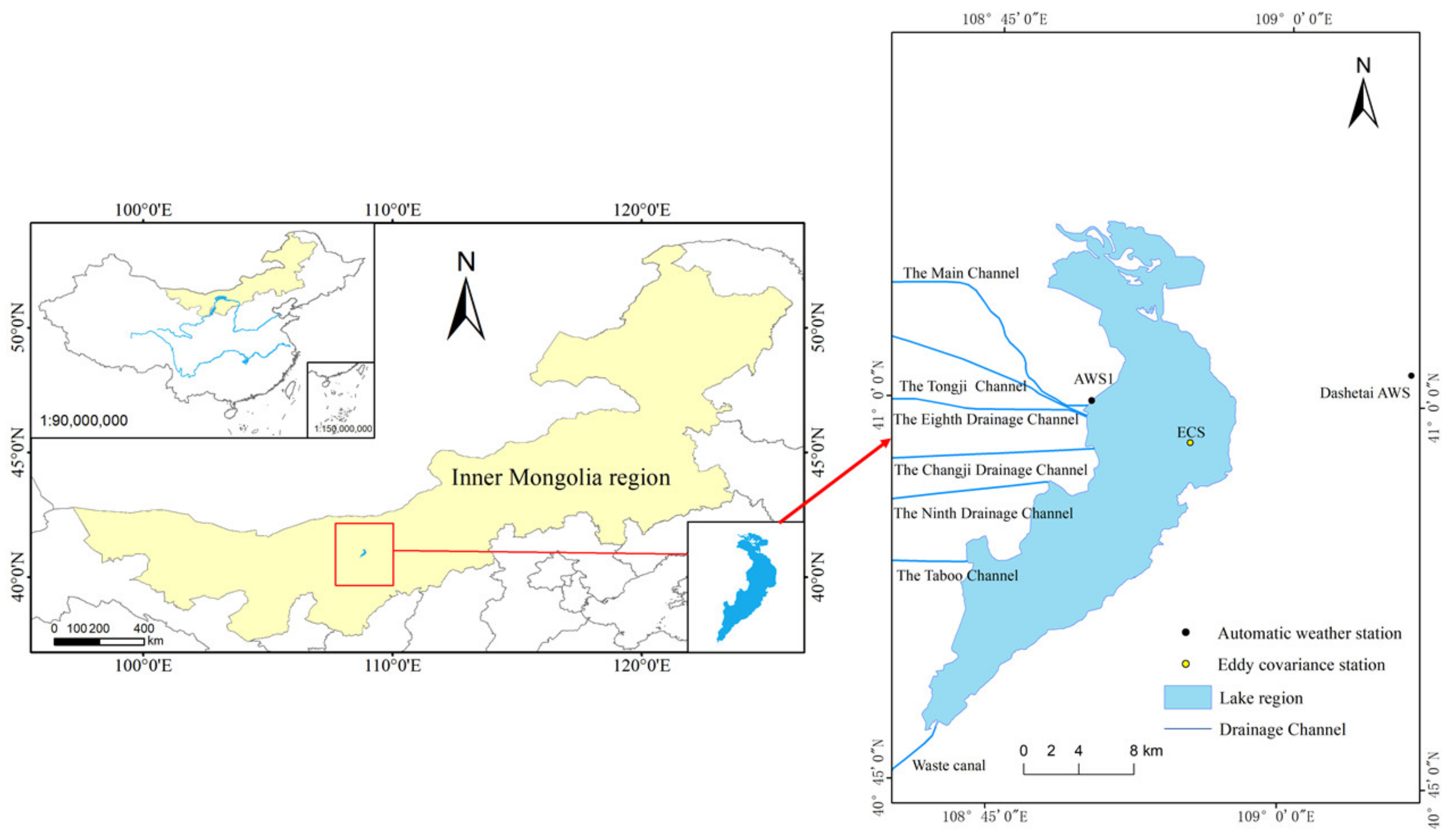
2.1. Study Area

Lake Wuliangsuhai (40°36′–41°03′ N, 108°43′–108°57′ E), located in Bayan Nur City, Inner Mongolia, is a plateau freshwater lake in the typical cold and arid region of northwest China. It is a unique and rare grass-type lake with multi-functional capabilities in desert and semi-desert areas worldwide. The lake covers an area of approximately 325 km2 (2019) and has a reservoir capacity of 2.5 to 3 × 10⁸ m3. The average elevation of the lake surface over the past decade has been 1018.5 m. The climate in the region is characterized by a mid-temperate continental monsoon, resulting in distinct seasonal changes. The winter is long, and the summer is short, with limited precipitation and high evaporation rates. The average annual precipitation level is reported to be 224.2 mm, while the average annual evaporation rate is 2300 mm. In late November, the onset of freezing temperatures occurred; the average water depth was 1.7 m, with ice thickness ranging between 0.3 to 0.6 m. In March, the thawing process commenced, culminating in a prolonged freeze–thaw cycle lasting approximately 4 to 5 months.

2.2. Sample Collection and Determination

2.2.1. Observation of Vorticity Flux

The Wuliangsuhai Ecological Station has deployed a high-frequency water quality monitoring system and an eddy covariance flux observation system (Figure 1) near the central water area of Wuliangsuhai (40°58′26.4″ N, 108°55′8.4″ E). The lake’s central water area is surrounded by waters that serve as a confluence of emergent, submerged, floating, and phytoplankton plants, which are minimally disturbed by human activities and provide an accurate representation of the water and air fluxes on the lake surface. The Wuliangsuhai eddy covariance flux observation system employs the IRGASON (Campbell, Inc., West Valley City, UT, USA, a probe height of 1.9 m), an integrated open-circuit eddy covariance system developed by Campbell in the United States. The vorticity system is connected to the CR3000 data collector (Campbell, Inc., West Valley City, UT, USA), which can generate high-frequency data at 10 Hz. From the analysis of the flux contribution area (Supplementary Materials Figure S1), it can be seen that the range of 50 m is the main contribution area of the flux.
In this study, all external biometeorological data are denoted by adding the suffix ‘1’ to the respective measurements. For example, the solar shortwave incident radiation is represented as SWIN1, TA represents the temperature measured by the vortex station, and TA1 represents the temperature measured by the weather station. In this study, EddyPro software (Version 7.0.9, LI-COR Inc., Lincoln, NE, USA) was utilized to preprocess the original 10 Hz flux data, resulting in the acquisition of a 30 min CO2 flux (FCO2) and H2O flux (FH2O). Pretreatment includes coordinate rotation [25], WPL correction [26], spectral correction [27], threshold elimination, quality control [28], etc. The FCO2 calculation is derived from the covariance term, temperature fluctuation correction term, and humidity correction term, whereas the FH2O calculation is from the covariance term and temperature fluctuation correction term [26,29,30]. The ET obtained by the vortex station was determined by multiplying the molecular weight of FH2O and converting it into the volume of liquid water using the following formulas:
F c = w ¯ c ¯ + w c ¯
FCO 2 :   F C = W ρ c ¯ + m a m v ρ c ¯ ρ a ¯ W ρ ν ¯ + 1 + ρ ν ¯ m a ρ a ¯ m v ρ c ¯ T ¯ W T ¯
FH 2 O :   F v = 1 + ρ v ¯ m a ρ a ¯ m v W ρ ν ¯ + ρ v ¯ W T ¯ T ¯
Note: The CO2 gas flux in Formula (1) is expressed as the sum of pulsation and average. Formula (2) is based on the pulsation of temperature and humidity and uses the Webb-Pearman-Leuning algorithm to calculate the CO2 gas flux. Similarly, Formula (3) is the H2O flux corrected by temperature fluctuation. where Fc is the CO2 flux; Fv is H2O flux; w ¯ is the average vertical wind speed (m/s); c ¯ is the average CO2 concentration (mmol/L); w is the fluctuating vertical wind speed (m/s); c is the fluctuating CO2 concentration (mmol/L); ρ c is the CO2 density fluctuation value (mg/L); ρ ν is the fluctuation value of water vapor density (mg/L); m a is the molar mass of air (g/mol); m v is the molar mass of water vapor (g/mol); ρ a is the fluctuation value of air density (mg/L); T ¯ is the average absolute temperature (k), and T is the fluctuating absolute temperature (k).

2.2.2. High-Frequency Meteorological–Water Quality Monitoring

Supplementary Materials (Table S1) provided in the support files list the names and abbreviations of the high-frequency meteorological–water quality monitoring indicators. The high-frequency water quality (half an hour) monitoring system of Lake Wuliangsuhai included the CS511-L dissolved oxygen sensor, CS547A-L conductivity sensor, OBS-3A turbidity sensor, 109-L water temperature sensor, and CS526-L pH sensor, as illustrated in Supplementary Materials (Figures S2 and S3). The water quality sensors were connected to a CR1000 data collector. The meteorological data used in this study were obtained from the HOBO automatic weather station located at the outlet of the AWS point on the west bank of the lake (41°00′ N, 108°50′ E), as depicted in Supplementary Materials (Figure S2). The collection frequency of the meteorological facility collector was 1 h, and it captured the temperature, air pressure, wind speed, wind direction, humidity, and solar shortwave radiation. Meteorological data were obtained through linear interpolation at a half-hourly frequency to synchronize the eddy and water quality monitoring data.

2.2.3. China’s General Water Surface Evaporation Formula C

The general formula C for water surface evaporation in China is denoted as Formula (4) [20]. The parameters of this formula were established based on the data gathered from 19 evaporation testing sites across China, including the Bayangaole station. Compared to the six alternative models utilized in the two climatic regions of China, this equation demonstrated a higher level of accuracy. Bayangaole station and Wuliangsuhai vortex station, both located in Bayan Nur City, exhibited comparable meteorological conditions.
E = 0.1 + 0.24 1 R H 2 1 2 ( e s e a ) u [ 0.85 u / ( u + 2 ) ]
Note: where E is the water surface evaporation (mm/h); u is wind speed (m/s); es is water surface saturated vapor pressure (hPa); ea is the actual water vapor pressure (hPa) of the air above the water surface; RH is relative humidity (%).

2.3. Data Processing

The analysis of fundamental data was performed using Microsoft Excel 2021 and SPSS 26.0. To assess the variation in environmental variables over time, principal component analysis was applied, and the difference in evaporation measured by in situ evaporation and evaporation pan was examined using independent sample testing. Additionally, Origin 2021 and Arcgis 10.7 were employed for data mapping and visualization of spatial distribution. A correlation heat map was generated using the ‘correlation plot’ package in OriginPro 2021 9.8.0.

3. Results

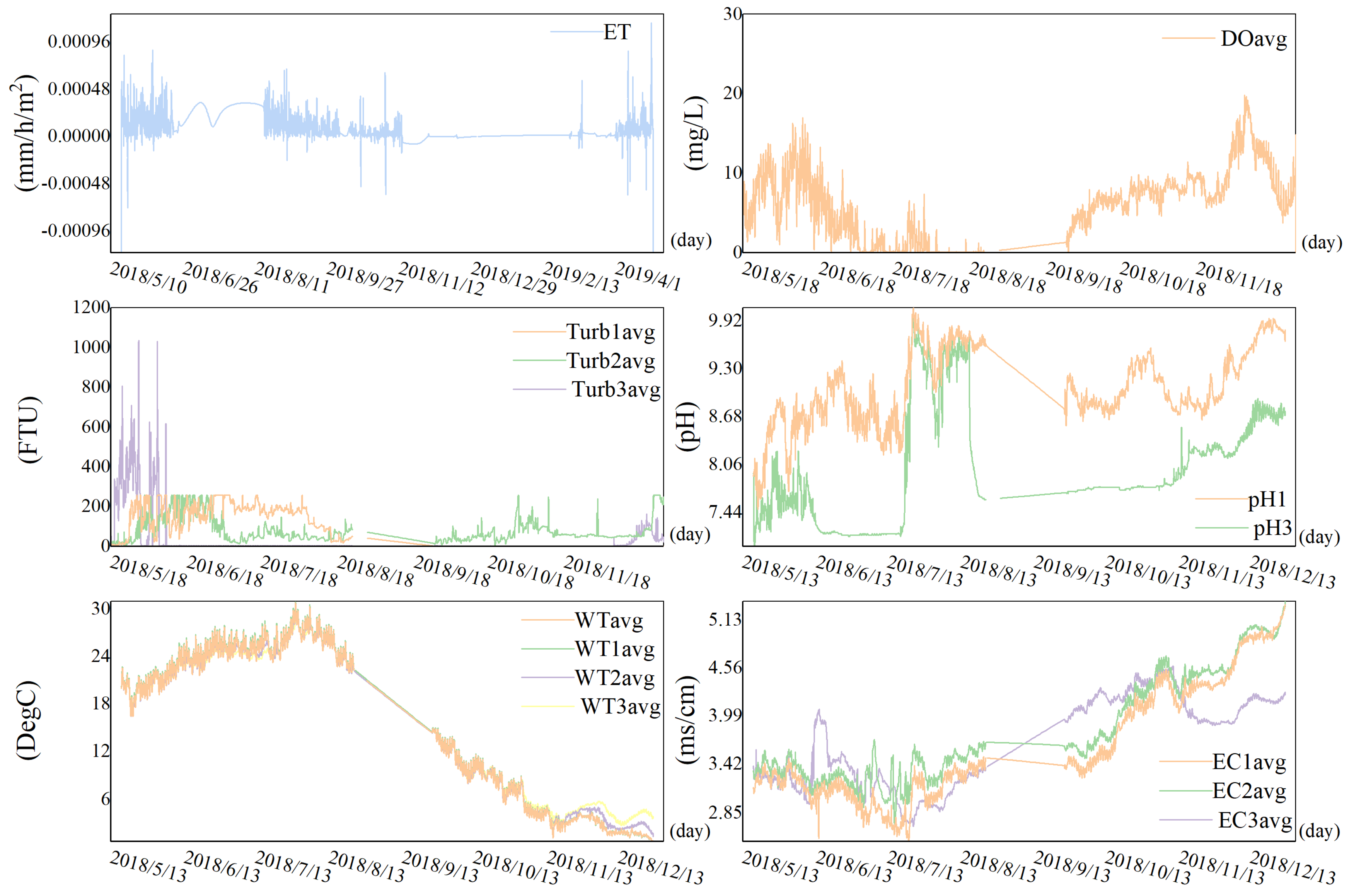
3.1. Variation Characteristics of FH2O (ET) and Environmental Factors Were Analyzed

3.1.1. High-Frequency Water Quality Determination Factor

The ET sampling period in Figure 2 is the overall scale, including the non-freezing period, initial ice period, freezing period, and thawing period (17 May 2018–25 April 2019). In addition, the other water quality index sampling periods are the non-freezing period-initial ice period (17 May 2018–28 December 2018). As depicted in Figure 2, the ET (18 June 2018–17 August 2018 data quality is not high is eliminated) value spanned from −0.0001 to 0.0005 mm/h/m2, with an average of 9.84 × 10⁻⁵ ± 12.77 × 10⁻⁵ mm/h/m2. Partial data on all water quality indicators are missing (24 August 2018–26 September 2018). The DOavg value ranged between 4.64 and 18.58 mg/L, with an average of 5.89 ± 4.39 mg/L. Additionally, the variation in water temperature followed a similar trend, varying in 0–30 °C, with a mean WTavg of 15.23 ± 9.79 °C.
There were notable modifications in the stratification of the three turbidity layers. The average Turb1avg value fluctuated between 0 and 259 FTU, with an average of 76.76 ± 92.09 FTU. The Turb2avg values varied between 0 and 250 FTU, with an average of 79.89 ± 62.47 FTU. Furthermore, the Turb3avg values ranged from 0 to 1110 FTU, with an average of 34.62 ± 107.48 FTU. Notably, the pH of the first layer was significantly higher than that of the third layer. The pH1 value exhibited a range from 7.50 to 10.10, with an average of 9.05 ± 0.49. Similarly, the pH3 value displayed a range from 7.01 to 9.97, with an average of 7.99 ± 0.71. The conductivity of the second layer consistently surpassed that of the first layer, whereas that of the third layer demonstrated significant variation. The EC1avg value ranged from 2.51 to 5.32 ms/cm, with an average of 3.65 ± 0.69 ms/cm. The EC2avg value ranged from 2.71 to 5.36 ms/cm, with an average of 3.83 ± 0.63 ms/cm. The EC3avg value exhibited a range of 2.69 to 4.59 ms/cm, with an average of 3.68 ± 0.53 ms/cm.

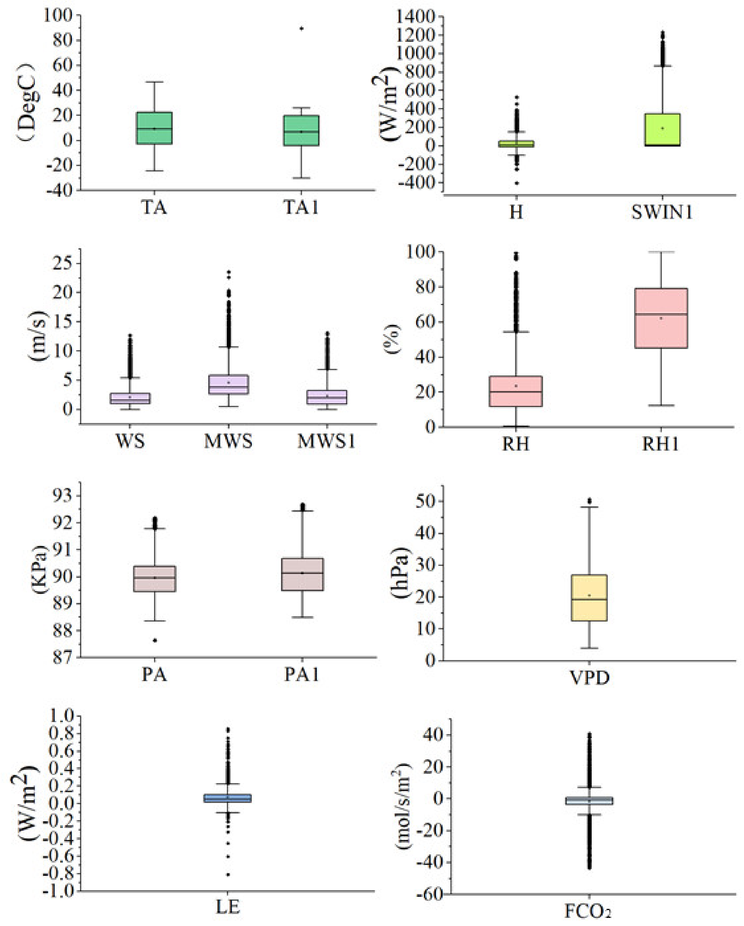
3.1.2. Meteorological Factors

The sampling periods of all meteorological indicators in Figure 3 are overall scales, including the non-freezing period, early freezing period, freezing period, and thawing period (17 May 2018–25 April 2019). From Figure 3, the temperature change range of the eddy station was larger than that of the meteorological station, with a TA value spanning −24.36 to 46.59 °C and an average value of 9.39 ± 14.71 °C. Additionally, the TA1 value has a range of −30.1 to 25.89 °C, with an average of 7.07 ± 12.32 °C. The H value at the eddy station exhibited a range of 0.6 to 530.26 W/m2, with an average of 28.99 ± 61.03 W/m2. The SWIN1 displayed a range of 0.6 to 1233.1 W/m2, with an average of 187.78 ± 265.16 W/m2. Furthermore, the wind speed change at the eddy station was greater than that of the meteorological station, with the WS ranging from 0.02 to 12.72 m/s and an average value of 2.05 ± 1.51 m/s. The MWS ranged from 0.51 to 23.56 m/s, with an average of 4.57 ± 2.64 m/s, while the MWS1 ranged from 0 to 13.09 m/s, with an average of 2.35 ± 1.93 m/s. Compared to the meteorological station, the change in the relative humidity at the eddy station was less pronounced. This could be due to the high wind speeds and dry air near the eddy station, as the RH value was predominantly below 30%, averaging 23.4 ± 26.8%. The RH1 ranged between 12.3% and 100%, with an average of 62.10 ± 20.59%. The air pressure at both the eddy and meteorological stations displayed similar changes. The PA ranged from 87.64 to 92.18 KPa, with an average of 899.60 ± 0.63 KPa. The PA1 was between 88.49 and 92.69 KPa, with an average of 90.13 ± 0.76 KPa. The VPD value ranged from 3.99 to 50.74 hPa, with an average of 20.45 ± 9.53 hPa. The LE ranged from −0.81 to 0.22 W/m2, with an average of 0.07 ± 0.09 W/m2. The FCO2 ranged from −429.96 to 792.42 mmol/s/m2, with an average of −1.66 ± 6.17 mmol/s/m2.

3.2. Influence of FH2O on Different Time Scales

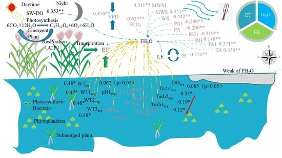
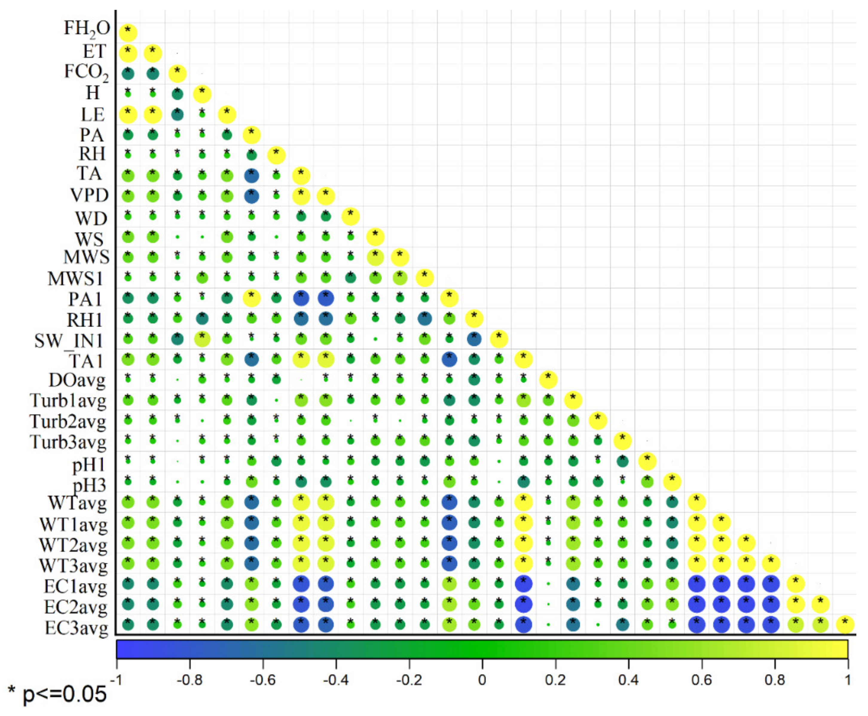
3.2.1. Correlation between Overall Scale FH2O and Meteorological Factors

In this study, environmental factors were categorized into meteorological factors and water quality factors and were examined from various perspectives. It has been widely accepted that FH2O between water and air on the lake surface is significantly affected by meteorology. Therefore, the relationship between FH2O and meteorological factors was first investigated in this study. Figure 4 illustrates that FH2O and FCO2 were moderately negatively correlated with meteorological factors. ET and LE were calculated using FH2O. Hence, they were completely correlated. They exhibited weak positive correlations with SWIN1, MWS1, VPD, TA1, TA, MWS, WS, and H and weak negative correlations with PA1, PA, and RH1. A high correlation between carbon and water fluxes was evident, and the carbon sink capacity of lakes was moderately positively correlated with FH2O. Shortwave radiation and wind-heat environmental factors enhanced the evapotranspiration process, thereby promoting the activity of FH2O. Conversely, the air pressure and humidity controlled the gas concentration in the atmosphere, thereby inhibiting the activity of FH2O. During the early freezing period, FH2O gradually became inactive and remained there until the melting ice period. Supplementary Materials (Table S2) demonstrates that the multiple linear regression equation derived from the regression analysis had a correlation coefficient of 0.734 with FH2O (May 2018–April 2019), indicating a significant correlation between FH2O and meteorological factors. In contrast to terrestrial ecosystems, FH2O in lake ecosystems was affected not only by precipitation and aquatic plant evapotranspiration but also by water surface evaporation and active material and energy exchange between the lake water and the atmosphere.

3.2.2. Correlation between FH2O and Environmental Factors in the Non-Freezing Period to Early Freezing Period

From Figure 4, the correlation between FH2O and pH1, as well as DOavg, was negligible and can be disregarded in the subsequent principal component analysis. However, because of the strong correlation between FH2O and environmental factors at the half-hour scale from the non-freezing period to the early freezing period, subsequent correlation analysis can be conducted. The F value of the Bartlett test was 0.000, indicating that the environmental factor data originated from a normally distributed population, whereas the KMO value was 0.872. This suggested that the data could be analyzed using principal component analysis. Extracting the principal component requires calculating the eigenvalues and eigenvectors of the matrix after obtaining the correlation coefficient matrix and, finally, calculating the cumulative contribution rate. The results of the principal component analysis are presented in Supplementary Materials (Tables S3–S5), and the principal components with eigenvalues greater than 1 were extracted. The extraction results indicated that the first six principal components accounted for a cumulative variance rate of 82.163%, implying that they contained all the information on the 26 indicators. The Zscore (FH2O) represented the standardized FH2O value.
The variance contribution rate of the first principal component was 47.593%, which was significantly higher than those of the other principal components. As shown in Supplementary Materials (Table S5), 13 environmental factors were closely related to the first principal component, as indicated by the factor load matrix of the principal components and environmental factors. The temperature indices, including water temperature and air temperature, exhibited a strong positive correlation with both WT1avg (r = 0.967) and TA1 (r = 0.959). Both water temperature and air temperature affected FH2O and were positively correlated. The salinity indices of the water body include conductivity (EC1avg, r = −0.911) and turbidity (Turb1avg, r = 0.654). Given that most returned water received by Wuliangsuhai annually passed through the saline-alkali land in the irrigation area, and local rainfall was minimal, the water body’s salinity was relatively high. Therefore, the first principal component can be considered as the temperature-salinity-pressure index. The environmental factors closely related to the second principal component were H, SWIN1, and MWS1, all of which were positively loaded. H was directly affected by solar shortwave radiation, and solar irradiation and wind blowing affected FH2O. The second principal component can be considered as the wind speed-sensible heat index. The environmental factors closely related to the third principal component were WS and MWS, and the third principal component can be considered as the wind speed index. The environmental factors closely related to the fourth principal component were ET and LE, and the evaporation of the lake water surface was strong. Therefore, the latent heat of evaporation affected the FH2O between water and air, and the fourth principal component can be considered as the evaporation-latent heat index. Turb2avg was an environmental factor closely related to the fifth principal component. Turbidity can reflect the suspended matter in the effluent. Suspended matter can absorb light and heat, thus affecting the evaporation of FH2O. The fifth principal component was the water purity index. The environmental factors closely related to the sixth principal component included PA1 and PA. Pressure indirectly affected FH2O by affecting wind speed and dew point. The sixth principal component was the air pressure index.

3.3. Evaporation Model from the Non-Freezing Period to the Early Freezing Period

3.3.1. FH2O Principal Component Regression Equation Model

The principal components, including Y1, Y2, Y3, Y4, Y5, and Y6, were derived by multiplying the principal component score factor by the square root of the eigenvalue, and the regression equation was determined by conducting a linear regression analysis of Zscore (FH2O) and the six principal components. As demonstrated in Supplementary Materials (Table S6), the correlation coefficient between the regression equation and Zscore (FH2O) was 0.93, while the R2 was 0.87, and the regression model hypothesis test was successfully passed. Moreover, as shown in Supplementary Materials (Table S7), the variance expansion factor VIF value of the principal component regression equation was less than 10, indicating no collinearity.
Therefore, the principal component regression equation can be obtained as
Z s c o r e F H 2 O = 0.039 + 0.159 × Y 1 + 0.159 × Y 2 + 0.161 × Y 3 + 0.472 × Y 4 0.107 × Y 5 0.028 × Y 6
The coefficient matrix for the principal component scores is presented in Supplementary Materials (Table S8). To express the regression equation utilizing standardized independent variables, the regression equation between the Zscore (FH2O) and each standardized environmental factor can be obtained through matrix operations involving the score coefficient matrix and regression coefficients of the six principal components. Finally, a regression equation for the Zscore (FH2O) was obtained:
Z s c o r e F H 2 O = 0.039 0.1586 × Z s c o r e ( F C O 2 ) + 0.019 × Z s c o r e ( S W I N 1 ) + 0.0074 × Z s c o r e ( P A ) + 0.0545 × Z s c o r e ( R H ) 0.0195 × Z s c o r e ( T A ) 0.0160 × Z s c o r e ( V P D ) + 0.0927 × Z s c o r e ( W S ) + 0.0483 × Z s c o r e ( M W S ) + 0.2321 × Z s c o r e ( E T ) 0.0108 × Z s c o r e ( H ) + 0.2321 × Z s c o r e ( L E ) 0.0416 × Z s c o r e ( M W S 1 ) + 0.0098 × Z s c o r e ( P A 1 ) + 0.0540 × Z s c o r e ( R H 1 ) 0.0083 × Z s c o r e ( T A 1 ) 0.0170 × Z s c o r e ( T u r b 1 a v g ) + 0.0216 × Z s c o r e ( T u r b 2 a v g ) 0.0634 × Z s c o r e ( T u r b 3 a v g ) + 0.0371 × Z s c o r e ( p H 3 ) 0.0063 × Z s c o r e ( W T a v g ) 0.0067 × Z s c o r e ( W T 1 a v g ) 0.0055 × Z s c o r e ( W T 2 a v g ) 0.0033 × Z s c o r e ( W T 3 a v g ) + 0.0161 × Z s c o r e ( E C 1 a v g ) + 0.0154 × Z s c o r e ( E C 2 a v g ) + 0.0181 × Z s c o r e ( E C 3 a v g )

3.3.2. FH2O Regression Model Validation

To assess the validity of the regression equation for the Zscore (FH2O), a simulated Zscore (FH2O) was derived using the regression equation and compared with the actual Zscore (FH2O). The results of this comparison are presented in Supplementary Materials (Tables S9 and S10).
According to Supplementary Materials (Figure S4), the fitting R square was 0.8057, indicating a high degree of fitting. This suggested that a principal component regression model can be established. The regression equation model results indicated that FH2O was directly or indirectly affected by meteorological and water quality factors. The exogenous driving factor was solar radiation, whereas the endogenous driving factor was the three-phase transformation of water. The analysis revealed that FH2O was primarily affected by the water and salt temperature indices, wind heat index, wind speed index, evaporation index, water purity index, and air pressure index. Among these factors, meteorological factors have a dominant impact on the FH2O. Of the water quality factors, FH2O exhibited a low correlation with pH1, pH3, and DOavg, whereas other water quality factors indirectly affected FH2O by influencing water evaporation and plant physiology.

4. Discussion

4.1. Lake Stratification and Water Quality Impact

Lake evaporation is a complex natural phenomenon that is affected by a multitude of interrelated and overlapping environmental factors. Current research generally categorizes these environmental impacts into two main groups: meteorological and characteristic lake conditions. Meteorological conditions include net radiation, wind speed, relative humidity, actual sunshine time, rainfall, runoff, air and water temperatures, and saturated vapor pressure. Lake characteristics mainly rely on factors such as location, depth, size, water temperature, salinity, transparency, geometry, surface area, and runoff [9,18,31,32]. However, the effects of diurnal variations, water quality, and stratification have been less considered. Moreover, the dependence of lake evaporation on environmental conditions has hindered the development of theoretical estimates [33]. According to the results of the Spearman correlation analysis presented in Figure 4, there was no significant correlation between ET and pH1avg or DOavg (p > 0.05) among the water quality factors.

4.1.1. No Stratified Change Water Quality Index

The average values of ET and the three-layer water temperature (r1 = 0.47; r2 = 0.48; r3 = 0.48) demonstrated a substantial positive correlation, whereas the average conductivity of the three layers (r1 = −0.42; r2 = −0.43; r3 = −0.41) exhibited a significant negative correlation. Owing to the shallow nature of Lake Wuliangsuhai, there was no stratification of water temperature and conductivity. The water temperature was an indicator of the movement energy of water molecules, with higher temperatures resulting in faster movement and stronger evaporation. The conductivity reflected the concentration of various ionic soluble salts in water, with higher concentrations resulting in greater conductivity. This was because salt-containing solutions formed a film on the water surface to inhibit evaporation.

4.1.2. With Stratified Changes in Water Quality Indicators

The correlation analysis revealed a notable negative correlation between ET and pH3avg (r = −0.14), and pH1avg was higher than pH3avg, with a larger range of change. This can be attributed to the rapid response of photosynthesis to radiation in a substantial number of aquatic plants, including phytoplankton, in the surface water body. In contrast, the bottom water body was less dependent on radiation, resulting in weak photosynthesis and stronger respiration. Photosynthesis, which consumed CO2, increased the pH value, while respiration, which produced CO2, reduced the pH value.
The relationship between the average value of ET and three-layer turbidity (r1 = 0.33; r2 = 0.19; r3 = 0.12) was significantly positive, with the correlation decreasing from the first layer to the third layer. Turbidity was a measure of the obstruction of lake water to light caused by insoluble substances. The penetration depth of radiation from surface water to bottom water can be determined by the turbidity associated with suspended organic and inorganic materials [9,34]. Phytoplankton exhibits light-driven properties, and submerged plants are predominantly located in surface water. Consequently, Turb1avg has a high correlation with ET. Insoluble substances can absorb radiation faster than lake water and subsequently transmit heat to the lake water, thereby accelerating evaporation. Numerous small and medium-sized lakes do not exhibit complete stratification in the vertical direction, and redistribution determines the distribution of biological communities [35].

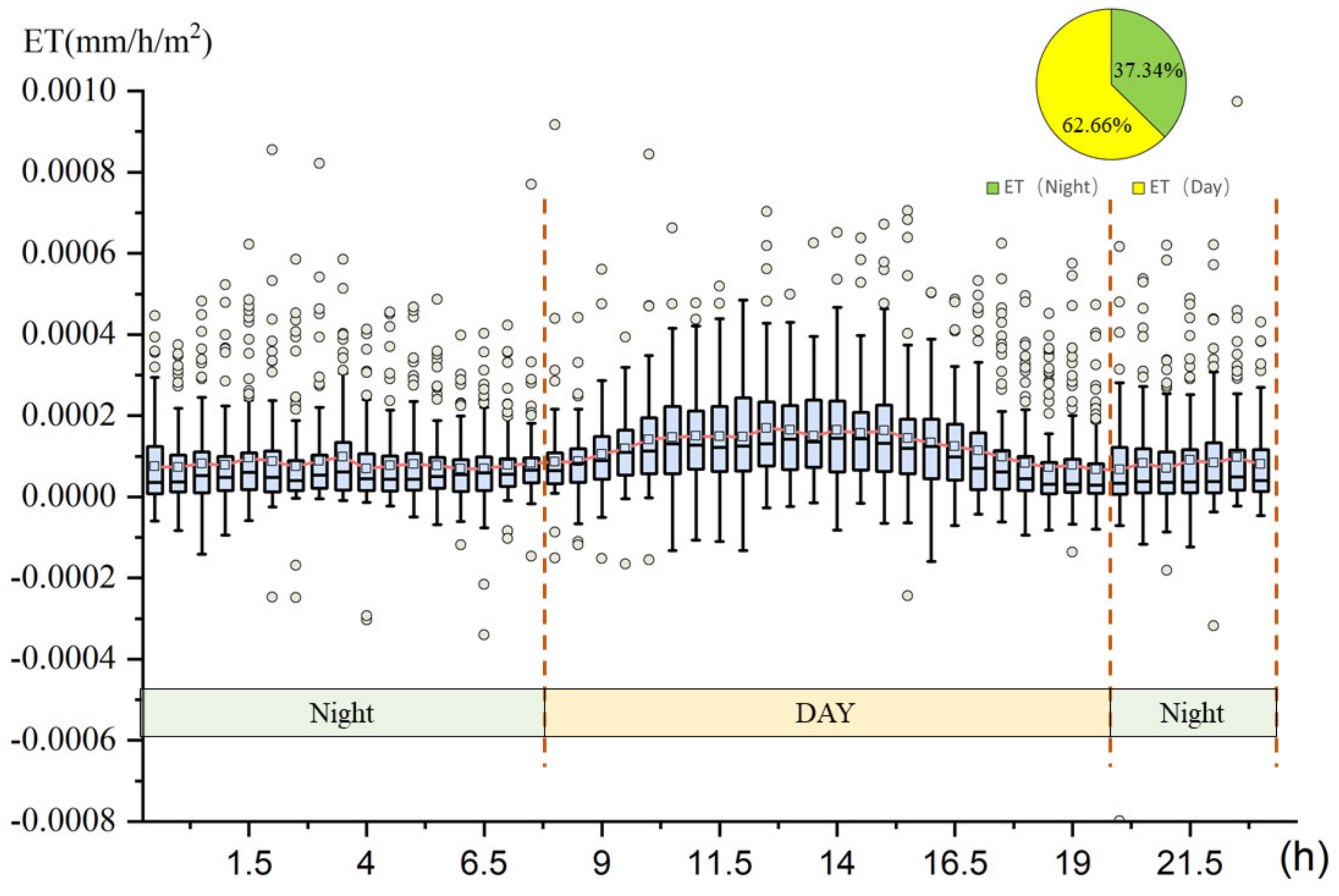
4.2. Diurnal Variation of ET in the Non-Freezing Period to Early Freezing Period

Expanding the spatial and temporal coverage of ET observations facilitates the identification of unknown or ambiguous ET processes, such as nighttime ET [3] and ice sheet decoupling. Nighttime ET is often underestimated, leading to an inaccurate estimation of total evaporation, whereas ice sheet decoupling effectively separates lake-air ET during winter and causes the formation of ice cover in the northern lakes of the Northern Hemisphere [36]. If nighttime ET was not considered, 37.34% of the total water surface evaporation of Lake Wuliangsuhai during the non-freezing period-early freezing period would be underestimated (Figure 5). Nighttime evaporation was a significant factor, accounting for 45% of the total evaporation water loss [9]. Therefore, the effect of ET at night cannot be ignored. At night, the ET was primarily affected by thermal inertia. On a daily to weekly scale, ET was affected by weather-scale models and was modulated by significant thermal hysteresis resulting from the high heat capacity of water [37]. The large heat capacity of water, combined with efficient vertical heat exchange, provided a lake with considerable heat-storage potential [38]. This, in turn, resulted in high thermal inertia for the lake, causing its temperature and turbulent exchange stage to differ from the surrounding land [39]. The degree of thermal hysteresis can depend mainly on the depth of the water [9,37]. The thermal lag time of shallow lakes is lower than that of deep lakes, and the water storage energy is more likely to respond to the water-air ET process.

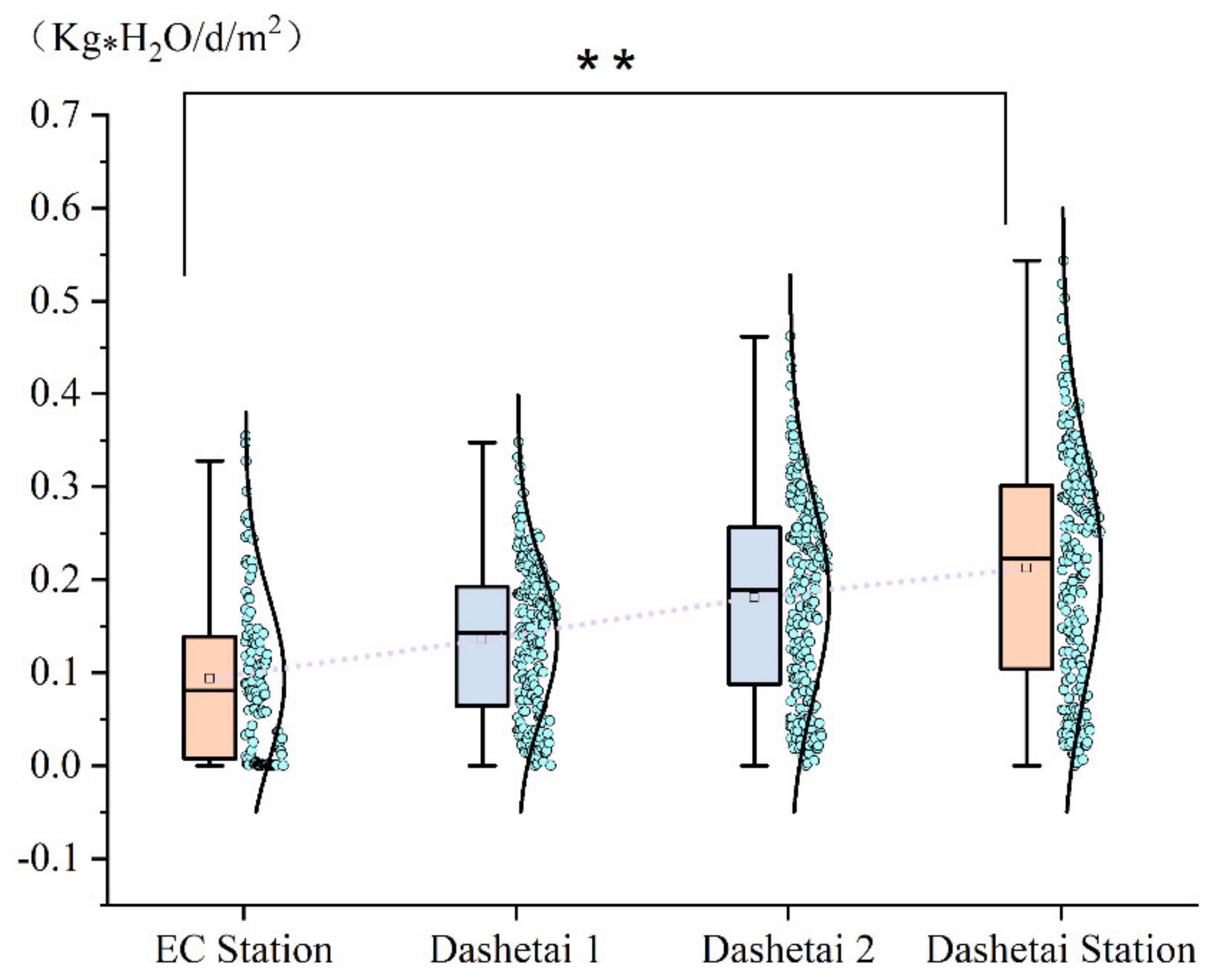
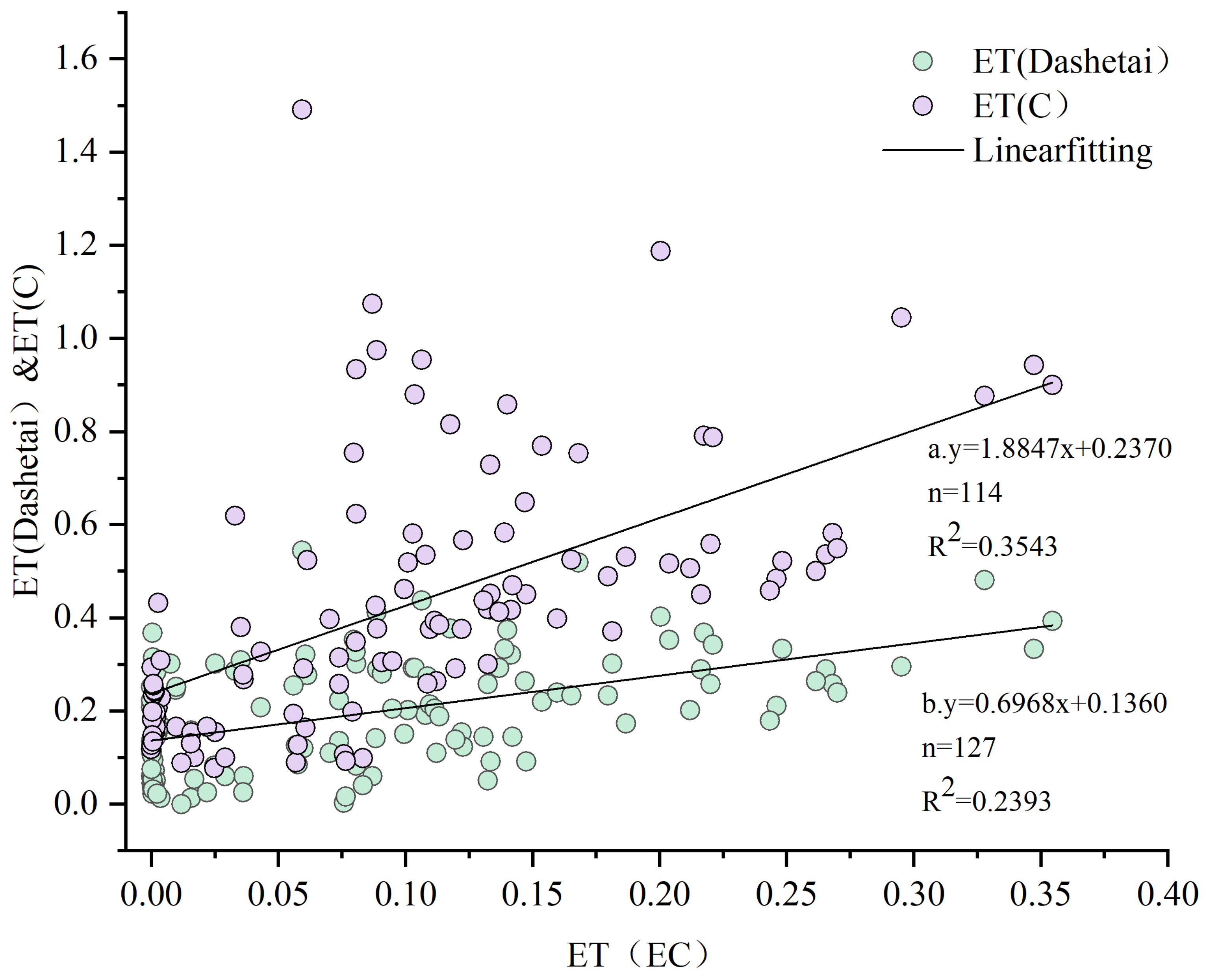
4.3. Comparison of the Model with Evaporation Dish Conversion and Regional Empirical C Formula Method

4.3.1. Comparison of Model and Evaporation Dish Conversion

Since the 18th century, the pan evaporation method has been employed to measure evaporation directly. In China, the majority of meteorological (hydrological) stations have installed 20 cm-diameter pans (and E-601 B pans). The potential evaporation of the water surface can be measured following the conversion of empirical parameters, which retains its relevance due to its classic and practical nature [3]. The eddy covariance technique is widely regarded as one of the most dependable methods for determining lake evaporation [3,20]. Traditionally, evaporation rate, as represented by evaporation capacity, has been employed to estimate actual evaporation. However, this method often results in an overestimation of lake water loss because the evaporation rate alone cannot accurately capture the magnitude of water loss. In a recent study on evaporative water loss in over 1.42 million lakes worldwide, Gang Zhao emphasized the importance of utilizing actual evaporation to assess lake-atmosphere interactions, thereby providing a comprehensive evaluation of the role of global lakes in the climate system [10].
Water surface evaporation is an essential component of the water cycle and balance in natural ecosystems during non-freezing and early freezing periods. Owing to the unique climate characteristics of cold and arid regions, which feature limited precipitation and strong evaporation, it is of utmost importance to accurately assess lake water surface evaporation. To facilitate a more accurate comparison and analysis of the evaporation values measured by the eddy station and Dashetai meteorological station, it is necessary to determine the distance between the two stations, which stands at 24.5 km. This study examined the volume of evaporation per square meter. Supplementary Materials (Tables S11 and S12) present the results of independent sample tests of the average daily evaporation amounts measured by the eddy station and Dashetai station (41°1′15.6″ N, 109°8′5.28″ E), respectively. The findings revealed a difference between the in situ evaporation and evaporation measured by the meteorological station. According to the findings of Liang Guisheng et al. (2002), the multi-year average value of the pan evaporation conversion coefficient in arid and semi-arid regions of the Yellow River Basin was estimated to be between 0.634 and 0.677 [40]. Additionally, Xu Wenhao et al.’s research on lakes in the Ordos Plateau suggested that the lake water evaporation conversion coefficient was approximately 0.85 [15]. The evaporation value at the Dashetai Station was measured using an evaporation pan with a φ20 cm diameter evaporation pan. The Dashetai Station 1 was the calculated result of the evaporation of the Dashetai Station with a conversion coefficient of 0.64, and the Dashetai Station 2 was the calculated result of a conversion coefficient of 0.85. Figure 6 shows that the amount of evaporation water measured in situ by the eddy station was smaller than the amount of evaporation water obtained by the evaporation pan conversion method.
In this study, FH2O displayed an upward flux during most of the monitoring period, indicating that ET was the primary mechanism by which FH2O was transferred to the atmosphere. Eddy station measurements represent the combined evaporation of the water surface and plant transpiration, providing a more accurate representation of the actual state of the lake. By analyzing the evaporation data from Dashetai station, the period between non-glacial and early freezing periods (18 May to 30 November 2018) was estimated for Lake Wuliangsuhai. During this period, the cumulative evaporation was 1333.5 mm, and the lake covered an area of 325 km2. The total evaporation during the non-freezing period was estimated to be between 2.77 and 3.68 × 10⁸ m3, while the eddy station calculated 1.91 × 10⁸ m3. In 2018, the annual ecological water replenishment was 9.59 × 10⁸ m3, and the total annual outflow was 8.07 × 10⁸ m3.
The rate of evaporation on the surface of the water is affected by both wind-induced convection and thermally unstable free convection and is closely related to factors such as water heat storage, heat conduction, temperature stratification at the water-air interface, and turbulence characteristics. First, the measurement of evaporation using a land pan is subject to several limitations, such as the pan’s design, location, effects of vegetation [32,41], water input and leakage, regular cleaning and maintenance, lack of thermal inertia, and ice phenology [23]. In addition, the conversion coefficient used to calculate evaporation is affected by numerous factors and varies with seasonal changes [42,43].
There are three primary reasons why the in situ eddy measurements of evaporation water can be smaller than that of land surface evaporation.
(1)
The first reason is that the thermal conditions and energy dissipation significantly affect the accuracy of the measurements due to the:
(i)
The ability of a lake to absorb solar radiation is greater due to its larger albedo, which means that the energy is quickly dissipated and does not directly contribute to evaporation. Additionally, the high specific heat capacity of natural water bodies like lakes requires more heat to evaporate the same amount of water, resulting in less evaporation under the same thermal radiation.
(ii)
The land surface possesses a greater expanse than both the temperature and the diurnal temperature fluctuation of the lake. Additionally, it presents a more favorable condition for water vaporization.
(iii)
The transverse heat exchange within the evaporator enhances the evaporation rate.
(2)
The second reason is related to the specific conditions of the lake, such as:
(i)
Wuliangsuhai is abundant in emergent plants such as reeds. These plants can effectively block sunlight, thereby reducing evaporation from the water surface. In addition, they can condense the water vapor under their leaves to prevent evaporation.
(ii)
The salinity of lakes is higher than that of pans, and high salinity can reduce water activity, effectively inhibiting evaporation [44].
(3)
The third reason pertains to the wind power and steam conditions such as:
(i)
The relative humidity of the lake is higher than that of the pan, whereas the VPD is lower.
(ii)
Lake evaporation is controlled by wind-driven mixing and the vertical temperature gradient between the lake and the atmosphere. In contrast, the pan is easily fully mixed, and wind-driven mixing maintains its temperature uniformity of the pan [37,45,46,47].

4.3.2. Comparison of the Model with the Regional Empirical C Formula Method

From the range of lake evaporation processes depicted in Figure 7, ET (C) > ET (Dashetai) > ET (EC). During the non-freezing period to the early freezing period (18 May to 30 November 2018), the accumulated ET (C) was 424.2% higher than ET (EC) in Lake Wuliangsuhai. Because of the limitations of the lake’s water storage capacity, it is evident that ET (C) does not accurately represent the actual evaporation situation in Lake Wuliangsuhai. Despite this, the similarity between the ET (EC) and ET (C) trends was higher than that between ET (EC) and ET (Dashetai) (Figure 8). ET (C) was moderated by wind speed, saturated vapor pressure difference, and relative humidity, which led to an overestimation of lake evaporation and a more discrete result. Additionally, formula C was a regional empirical formula based on evaporation pan data from the evaporation station, which was also affected by the evaporation pan conversion algorithm. Upon comparing the values, the lake evaporation calculated using the C formula surpassed the water storage capacity of Lake Wuliangsuhai, indicating that the C formula was incapable of accurately capturing environmental variables. Although the evaporation dish conversion algorithm may occasionally overestimate the evaporation values, it remained relatively stable. Hence, by utilizing the evaporation measurements from the vortex station as a reference, re-calculating the evaporation dish conversion coefficient can enhance the accuracy of the evaporation dish conversion algorithm. In future studies on lake evaporation, incorporating eddy station data with the evaporation dish conversion algorithm can expand the spatial scale while maintaining accuracy.

5. Conclusions

This study investigated the evaporation and environmental parameters of Lake Wuliangsuhai through high-frequency meteorological and water quality monitoring from May 2018 to April 2019. This study shows that the real water surface evaporation of the lake is much smaller than the measured value by the evaporation pan conversion method and the regional empirical C formula method. The amount of evaporated water obtained by the pan method is 1.45~1.92 times that of the model method. The regional empirical C formula method is more than four times that of the model method and exceeds the storage capacity limit. It can be seen that low-frequency and less environmental index observations will overestimate real lake evaporation. Lake evaporation is affected by meteorological–water quality constraints, and water quality indicators significantly related to ET are also affected by lake stratification. Considering the multiple effects of meteorological and water quality can improve the accuracy of describing lake ET. There was a significant diurnal variation of ET during the non-freezing period to the early glacial period, which was affected by the thermal inertia lag. Nighttime ET accounted for a higher proportion of total evaporation loss. Therefore, nighttime ET should be added to the evaluation of lake ET. In future research, more meteorological and water quality monitoring indicators should be added to continue to improve the accuracy of the model. It is necessary to increase the in situ lake surface evaporation pan monitoring to better compare the amount of evaporation water. In addition, evaporation Modelling should be carried out in other lakes or waters to break the regional confinement. The research results can provide new insights into lake evaporation observations in the middle and high latitudes of cold, arid, and semi-arid regions of China.

Supplementary Materials

The following supporting information can be downloaded at: https://www.mdpi.com/article/10.3390/w16040578/s1.

Author Contributions

Y.S.: Conceptualization, Methodology, Investigation, Writing—Original Draft. X.S.: Writing—Review and Editing. S.Z.: Validation, Formal analysis. G.L.: Data Curation, Formal analysis. B.S.: Data Curation, Writing—Review and Editing. J.H.: Writing—Review and Editing, Supervision. All authors have read and agreed to the published version of the manuscript.

Funding

This research was funded by the National Natural Science Foundation of China (grant number 52260028; 52060022; 5236914; 52260029; 52160021); the Inner Mongolia Autonomous Region Science and Technology Plan (grant number 2021GG0089), And The APC was funded by Xiaohong Shi.

Data Availability Statement

The authors do not have permission to share data.

Conflicts of Interest

The authors declare that they have no known competing financial interests or personal relationships that could have appeared to influence the work reported in this paper.

References

  1. Jing, S.; Xiao, W.; Wang, J. Evaporation variability and its control factors of Lake Taihu from 1958 to 2017. J. Lake Sci. 2022, 34, 1697–1711. [Google Scholar] [CrossRef]
  2. Oki, T.; Kanae, S. Global hydrological cycles and world water resources. Science 2006, 313, 1068–1072. [Google Scholar] [CrossRef]
  3. Liu, Y.; Qiu, G.; Zhang, H.; Yang, Y.; Zhang, Y.; Wang, Q.; Zhao, W.; Jia, L.; Ji, X.; Xiong, Y.; et al. Shifting from homogeneous to heterogeneous surfaces in estimating terrestrial evapotranspiration: Review and perspectives. Sci. China Earth Sci. 2022, 65, 197–214. [Google Scholar] [CrossRef]
  4. Liu, H.; Zhang, Y.; Liu, S.; Jiang, H.; Sheng, L.; Williams, Q.L. Eddy covariance measurements of surface energy budget and evaporation in a cool season over southern open water in Mississippi. J. Geophys. Res. Atmos. 2009, 114. [Google Scholar] [CrossRef]
  5. Walter, K.M.; Zimov, S.A.; Chanton, J.P.; Verbyla, D.; Chapin, F.S., III. Methane bubbling from Siberian thaw lakes as a positive feedback to climate warming. Nature 2006, 443, 71–75. [Google Scholar] [CrossRef] [PubMed]
  6. Long, Z.; Perrie, W.; Gyakum, J.; Caya, D.; Laprise, R. Northern lake impacts on local seasonal climate. J. Hydrometeorol. 2007, 8, 881–896. [Google Scholar] [CrossRef]
  7. Yao, X.; Yang, K.; Zhou, X.; Wang, Y.; Lazhu Chen, Y.; Lu, H. Surface friction contrast between water body and land enhances precipitation downwind of a large lake in Tibet. Clim. Dyn. 2021, 56, 2113–2126. [Google Scholar] [CrossRef]
  8. Xu, L.; Liu, H.; Du, Q.; Wang, L.; Yang, L.; Sun, J. Differences of atmospheric boundary layer characteristics between pre-monsoon and monsoon period over the Erhai Lake. Theor. Appl. Climatol. 2019, 135, 305. [Google Scholar] [CrossRef]
  9. Bai, P.; Wang, Y. The Importance of Heat Storage for Estimating Lake Evaporation on Different Time Scales: Insights from a Large Shallow Subtropical Lake. Water Resour. Res. 2023, 59, e2023WR035123. [Google Scholar] [CrossRef]
  10. Zhao, G.; Li, Y.; Zhou, L.; Gao, H. Evaporative water loss of 1.42 million global lakes. Nat. Commun. 2022, 13, 3686. [Google Scholar] [CrossRef]
  11. Ritchie, H.; Roser, M. Water Use and Stress, Our World in Data. 2017. Available online: https://ourworldindata.org/water-use-stress (accessed on 6 November 2023).
  12. Zhao, G.; Gao, H.; Cai, X. Estimating lake temperature profile and evaporation losses by leveraging MODIS LST data. Remote Sens. Environ. 2020, 251, 112104. [Google Scholar] [CrossRef]
  13. Ito, Y.; Momii, K. Potential effects of climate changes on evaporation from a temperate deep lake. J. Hydrol. Reg. Stud. 2021, 35, 100816. [Google Scholar] [CrossRef]
  14. Pérez, A.; Lagos, O.; Lillo-Saavedra, M.; Souto, C.; Paredes, J.; Arumí, J.L. Mountain lake evaporation: A comparative study between hourly estimations models and in situ measurements. Water 2020, 12, 2648. [Google Scholar] [CrossRef]
  15. Xu, W.; Wang, X.; Zhang, J. Research on in-situ test of lake evaporation in the Ordos Plateau. Hydrogeol. Eng. Geol. 2019, 46, 1000–3665. [Google Scholar] [CrossRef]
  16. El-Mahdy ME, S.; El-Abd, W.A.; Morsi, F.I. Forecasting lake evaporation under a changing climate with an integrated artificial neural network model: A case study Lake Nasser, Egypt. J. Afr. Earth Sci. 2021, 179, 104191. [Google Scholar] [CrossRef]
  17. Zhou, W.; Wang, L.; Li, D.; Leung, L.R. Spatial Pattern of Lake Evaporation Increases under Global Warming Linked to Regional Hydroclimate Change. Commun. Earth Environ. 2021, 2, 255. [Google Scholar] [CrossRef]
  18. Wang, W.; Lee, X.; Xiao, W.; Liu, S.; Schultz, N.; Wang, Y.; Zhang, M.; Zhao, L. Global lake evaporation accelerated by changes in surface energy allocation in a warmer climate. Nat. Geosci. 2018, 11, 410–414. [Google Scholar] [CrossRef]
  19. Wang, B.; Ma, Y.; Su, Z.; Wang, Y.; Ma, W. Quantifying the evaporation amounts of 75 high-elevation large dimictic lakes on the Tibetan Plateau. Sci. Adv. 2020, 6, eaay8558. [Google Scholar] [CrossRef]
  20. Cui, Y.; Liu, Y. Advances in observation and calculation of lake evaporation. J. Lake Sci. 2023, 35, 1501–1515. [Google Scholar] [CrossRef]
  21. Phillips, R.C.; Saylor, J.R.; Kaye, N.B.; Gibert, J.M. A multi-lake study of seasonal variation in lake surface evaporation using MODIS satellite-derived surface temperature. Limnology 2016, 17, 273–289. [Google Scholar] [CrossRef]
  22. Momii, K.; Ito, Y. Heat budget estimates for lake Ikeda, Japan. J. Hydrol. 2008, 361, 362–370. [Google Scholar] [CrossRef]
  23. Li, X.Y.; Ma, Y.J.; Huang, Y.M.; Hu, X.; Wu, X.C.; Wang, P.; Li, G.Y.; Zhang, S.Y.; Wu, H.W.; Jiang, Z.Y.; et al. Evaporation and surface energy budget over the largest high-altitude saline lake on the Qinghai-Tibet Plateau. J. Geophys. Res. Atmos. 2016, 121, 10–470. [Google Scholar] [CrossRef]
  24. Assouline, S.; Tyler, S.W.; Tanny, J.; Cohen, S.; Bou-Zeid, E.; Parlange, M.B.; Katul, G.G. Evaporation from three water bodies of different sizes and climates: Measurements and scaling analysis. Adv. Water Resour. 2008, 31, 160–172. [Google Scholar] [CrossRef]
  25. Chapin, F.S., III; McGuire, A.D.; Randerson, J.; Pielke, R.; Baldocchi, D.; Hobbie, S.E.; Roulet, N.; Eugster, W.; Kasischke, E.; Rastetter, E.B.; et al. Arctic and boreal ecosystems of western North America as components of the climate system. Glob. Change Biol. 2000, 6, 211–223. [Google Scholar] [CrossRef]
  26. Webb, E.K.; Pearman, G.I.; Leuning, R. Correction of flux measurements for density effects due to heat and water vapour transfer. Q. J. R. Meteorol. Soc. 1980, 106, 85–100. [Google Scholar] [CrossRef]
  27. McDermitt, D.; Burba, G.; Xu, L.; Anderson, T.; Komissarov, A.; Riensche, B.; Schedlbauer, J.; Starr, G.; Zona, D.; Oechel, W.; et al. A new low-power, open-path instrument for measuring methane flux by eddy covariance. Appl. Phys. B 2011, 102, 391–405. [Google Scholar] [CrossRef]
  28. Foken, T.; Göockede, M.; Mauder, M.; Mahrt, L.; Amiro, B.; Munger, W. Post-field data quality control. In Handbook of Micrometeorology: A Guide for Surface Flux Measurement and Analysis; Springer: Dordrecht, The Netherlands, 2004; pp. 181–208. [Google Scholar]
  29. Massman, W.J.; Lee, X. Eddy covariance flux corrections and uncertainties in long-term studies of carbon and energy exchanges. Agric. For. Meteorol. 2002, 113, 121–144. [Google Scholar] [CrossRef]
  30. Leuning, R.A.Y.; Judd, M.J. The relative merits of open-and closed-path analysers for measurement of eddy fluxes. Glob. Change Biol. 1996, 2, 241–253. [Google Scholar] [CrossRef]
  31. Finch, J.; Hall, R. Estimation of Open Water Evaporation: A Review of Methods; Environment Agency: Bristol, UK, 2001.
  32. Aydin, H.; Karakuş, H. Estimation of evaporation for Lake Van. Environ. Earth Sci. 2016, 75, 1275. [Google Scholar] [CrossRef]
  33. Antonopoulos, V.Z.; Gianniou, S.K.; Antonopoulos, A.V. Artificial neural networks and empirical equations to estimate daily evaporation: Application to lake Vegoritis, Greece. Hydrol. Sci. J. 2016, 61, 2590–2599. [Google Scholar] [CrossRef]
  34. Liu, H.; Zhang, Q.; Dowler, G. Environmental controls on the surface energy budget over a large southern inland water in the United States: An analysis of one-year eddy covariance flux data. J. Hydrometeorol. 2012, 13, 1893–1910. [Google Scholar] [CrossRef]
  35. Boehrer, B.; Schultze, M. Stratification of lakes. Rev. Geophys. 2006, 46. [Google Scholar] [CrossRef]
  36. Wang, W.; Xiao, W.; Cao, C.; Gao, Z.; Hu, Z.; Liu, S.; Shen, S.; Wang, L.; Xiao, Q.; Xu, J.; et al. Temporal and spatial variations in radiation and energy balance across a large freshwater lake in China. J. Hydrol. 2014, 511, 811–824. [Google Scholar] [CrossRef]
  37. Xiao, K.; Griffis, T.J.; Baker, J.M.; Bolstad, P.V.; Erickson, M.D.; Lee, X.; Wood, J.D.; Hu, C.; Nieber, J.L.; Nieber, J.L. Evaporation from a temperate closed-basin lake and its impact on present, past, and future water level. J. Hydrol. 2018, 561, 59–75. [Google Scholar] [CrossRef]
  38. Nordbo, A.; Launiainen, S.; Mammarella, I.; Lepparanta, M.; Huotari, J.; Ojala, A.; Vesala, T. Long-term energy flux measurements and energy balance over a small boreal lake using eddycovariance technique. J. Geophys. Res. 2011, 116. [Google Scholar] [CrossRef]
  39. Li, Z.; Lyu, S.; Ao, Y.; Wen, L.; Zhao, L.; Wang, S. Long-term energy flux and radiation balance observations over Lake Ngoring, Tibetan Plateau. Atmos. Res. 2015, 155, 13–25. [Google Scholar] [CrossRef]
  40. Liang, G.; Lu, S.; Cai, M.J. Conversion coefficient and climate calculation of small evaporator in arid area. J. Yellow River Conserv. Tech. Inst. 2002, 3, 37–39. [Google Scholar] [CrossRef]
  41. Allen, R.G.; Tasumi, M. Evaporation from American Falls Reservoir in Idaho via a combination of Bowen ratio and eddy covariance. In Impacts of Global Climate Change; ASCE: Reston, VA, USA, 2005; pp. 1–17. [Google Scholar] [CrossRef]
  42. Zhao, X.; Li, M.; Wang, S.; Liu, Y. Comparison of actual water evaporation and pan evaporation in summer over the Lake Poyang, China. J. Lake Sci. 2015, 27, 343–351. [Google Scholar] [CrossRef]
  43. Grismer, M.E.; Orang, M.; Snyder, R.; Matyac, R. Pan evaporation to reference evapotranspiration conversion methods. J. Irrig. Drain. Eng. 2002, 128, 180–184. [Google Scholar] [CrossRef]
  44. Mor, Z.; Assouline, S.; Tanny, J.; Lensky, I.M.; Lensky, N.G. Effect of water surface salinity on evaporation: The case of a diluted buoyant plume over the Dead Sea. Water Resour. Res. 2018, 54, 1460–1475. [Google Scholar] [CrossRef]
  45. Blanken, P.D.; Rouse, W.R.; Culf, A.D.; Spence, C.; Boudreau, L.D.; Jasper, J.N.; Kochtubajda, B.; Schertzer, W.M.; Marsh, P.; Verseghy, D. Eddy covariance measurements of evaporation from Great Slave Lake, Northwest Territories, Canada. Water Resour. Res. 2000, 36, 1069–1077. [Google Scholar] [CrossRef]
  46. Martínez, J.M.M.; Alvarez, V.M.; González-Real, M.M.; Baille, A. A simulation model for predicting hourly pan evaporation from meteorological data. J. Hydrol. 2006, 318, 250–261. [Google Scholar] [CrossRef]
  47. Roderick, M.L.; Rotstayn, L.D.; Farquhar, G.D.; Hobbins, M.T. On the attribution of changing pan evaporation. Geophys. Res. Lett. 2007, 34, 17. [Google Scholar] [CrossRef]
Figure 1. Geographic distribution map of sampling points in Lake Wuliangsuhai.
Water 16 00578 g001
Figure 2. High−frequency water quality changes.
Water 16 00578 g002
Figure 3. High−frequency meteorological changes.
Water 16 00578 g003
Figure 4. Correlation of H2O fluxes with environmental factors during the non−freezing period to early freezing period (p < 0.05). Note: The dot size is proportional to the correlation, that is, the larger the circle, the higher the correlation.
Water 16 00578 g004
Figure 5. Instantaneous ET flux changes.
Water 16 00578 g005
Figure 6. Comparison of EC station and evaporation dish discounting methods. Note: orange represents site data, blue represents converted data; ‘**’ represents (p < 0.01), indicating that there is a significant difference between the two site data.
Water 16 00578 g006
Figure 7. ET (EC) vs. ET (C) and ET (Dashetai).
Water 16 00578 g007
Figure 8. ET (EC) fitted with ET (C) and ET (Dashetai).
Water 16 00578 g008
Disclaimer/Publisher’s Note: The statements, opinions and data contained in all publications are solely those of the individual author(s) and contributor(s) and not of MDPI and/or the editor(s). MDPI and/or the editor(s) disclaim responsibility for any injury to people or property resulting from any ideas, methods, instructions or products referred to in the content.

