Water Quality Inversion of a Typical Rural Small River in Southeastern China Based on UAV Multispectral Imagery: A Comparison of Multiple Machine Learning Algorithms

Abstract

Remote sensing technology applications for water quality inversion in large rivers are common. However, their application to medium/small-sized water bodies within rural areas is limited due to the low spatial resolution of remote sensing images. In this work, a typical small rural river was selected, and high-resolution unmanned aerial vehicle (UAV) multispectral images and ground monitoring data of the river were obtained. Then, a comparative analysis of three univariate regression models and nine machine learning models (Ridge Regression (RR), Support Vector Regression (SVR), Grid Search Support Vector Regression (GS-SVR), Random Forest (RF), Grid Search Random Forest (GS-RF), eXtreme Gradient Boosting (XGBoost), Deep Neural Networks (DNN), Convolutional Neural Networks (CNN), and Catboost Regression (CBR)) for their accuracy in the prediction of turbidity (TUB), total nitrogen (TN), and total phosphorus (TP) was performed. TUB can be achieved by simple statistical regression models. The CBR model exhibited the best performance for the three index inversions on the test set evaluation metrics: R² (0.90~0.92), RMSE (7.57 × 10⁻³~1.59 mg/L), MAE (0.01~1.30 mg/L), RPD (3.21~3.56), and NSE (0.84~0.92). The water pollution of the study area was closely related to its land-use pattern, excessive and irrational fertilizer application, and distribution of pollutant outlets.

1. Introduction

Inland water bodies are pivotal freshwater reservoirs, wielding substantial significance not only in terms of their water resource potential but also in their capacity to facilitate vital functions such as irrigation, flood control, and environmental conservation [1]. Medium/small-sized water bodies are an important component of inland water bodies. In China, there exist more than 40,000 medium/small-sized water bodies with a water area of less than 3000 square kilometers (http://www.mwr.gov.cn/ (accessed on 30 October 2023)). This substantial quantity includes a significant proportion of rural rivers, predominantly ensconced within densely inhabited villages, agricultural lands, and aquaculture facilities. Owing to the utilization of pesticides and chemical fertilizers, the discharge of domestic sewage originating from rural communities, and the unmitigated runoff of livestock and poultry waste during the rainy season, the water quality of these small and medium-sized rural rivers faces severe threats. Consequently, it is imperative to conduct sustained, long-term water quality monitoring for these watercourses.

Traditional water quality tests, e.g., COD (Chemical Oxygen Demand), TN (total nitrogen), and TP (total phosphorus), can obtain precise values of water quality parameters, However, to comprehensively measure the quality of the water environment, it is often necessary to carry out chemical analyses of multiple water quality indicators, which is time consuming, significantly increases economic costs, and ultimately obtains only discrete data on the quality of river water [2]. Furthermore, water quality assessment results from individual sampling points are considered inadequate in providing a comprehensive representation of the pollutant distribution within an entire water body. There is an urgent need for an alternative approach that can reduce economic costs, enhance time efficiency, and comprehensively capture the spatiotemporal distribution characteristics of water bodies. Recently, remote sensing technologies have been introduced as novel monitoring approaches for water environment surveillance [3,4,5,6,7,8], ushering in new opportunities. Among the emerging remote sensing methods is satellite remote sensing, which enables the monitoring of vast water areas. However, the majority of satellite images exhibit low spatial resolution, protracted revisit periods, and vulnerability to atmospheric cloud interference, thereby impeding their suitability for real-time monitoring of medium/small-sized water bodies and presenting certain limitations [9]. With the progress of UAV technologies and sensors, UAV remote sensing has gradually emerged as an applicable methodology in water environment monitoring for its enhanced mobility, flexibility, and ease of operation, featuring high spatial resolution. It is especially suitable for the monitoring of medium/small-sized water bodies.

Water quality inversion methods offer an effective means to monitor variations in river water quality, enabling the spatial representation of pollutant distributions within river systems. Traditional water quality inversion models primarily rely on statistical regression analysis, which, while being straightforward, often exhibits lower fitting accuracy. Numerous studies have indicated that machine learning can capture the intricate nonlinear mapping relationships between remote sensing reflectance and water quality parameters [10,11,12,13,14,15,16,17,18,19]. This significantly addresses the underfitting issues encountered in traditional regression models, opening up new possibilities for water quality inversion. For instance, Tan et al. [20] established three machine learning inversion models—Neural Network (NN), Random forest (RF), and Support Vector Regression (SVR)—for TN and TP metrics based on Sentine-2 data and measured data of Minjiang River (Sichuan, China), and concluded that RF had good potential for application. Li et al. [21] utilized Landsat 8 satellite remote sensing image data to establish a machine learning-based inversion model for TN prediction in Donghu Lake, with a high R² of 0.88. Wang et al. [22] inverted the TUB concentration of inland aquaculture water based on UAV and the Dynamic Network Surgery-Deep Neural Networks (DNS-DNN) algorithm, and the RMSE was controlled within 0.18. Sharafti et al. [23] employed three novel ensemble machine learning models—Ada Boost Regression (ABR), Gradient Boost Regression (GBR), and RF—to predict water quality parameters such as five-day biochemical oxygen demand (BOD₅) and chemical oxygen demand (COD).

Currently, instances of water quality inversion are not uncommon, and extensive research has been conducted on methods for water quality inversion in large bodies of water such as lakes, rivers, reservoirs, and urban landscape waterways [24,25,26,27,28]. Successful outcomes have been achieved in lake water quality inversion by Li et al. [29], Fu et al. [30], and Wang et al. [31], while research by Tan et al. [20], Cao et al. [32], and Ding et al. [33] on large river water quality inversion has produced relevant results. Simultaneously, reservoir water quality inversion has been accomplished by He et al. [15], Qian et al. [34], and Jiang et al. [35]. However, in the realm of small to medium-sized rivers, the existing focus tends to be more on urban rivers [16,24,36], with relatively limited exploration of rural rivers. Small rural water bodies, characterized by complex composition, limited areas, and narrow water surfaces, are highly susceptible to significant environmental influences, leading to increased water environment instability. These rivers often play a crucial role in agricultural irrigation and fish farming, highlighting the urgency for developing stable and accurate water quality inversion models, especially considering the general absence of automatic water quality monitoring equipment in rural rivers. Furthermore, existing research has predominantly concentrated on the inversion of optical-sensitive parameters such as Chlorophyll (Chla) and TUB [37,38,39,40,41,42], whereas the exploration of nonoptical sensitive parameters (TN/TP) remains comparatively limited. Nonetheless, nonoptical sensitive parameters are closely tied to pollutant and nutrient levels in water, making them crucial for assessing the status of aquatic ecosystems. Therefore, for a comprehensive understanding of the status of water bodies, there is an urgent need for accurate, timely, and dynamic monitoring of nonoptical sensitive parameters in small/medium-sized rural rivers with the help of remote sensing technology.

In this context, the objectives of this study are as follows: (1) to compare the effectiveness of nine ML methods for predicting three water quality indicators (i.e., TUB, TN, TP) in small/medium-sized rural rivers; (2) to explore the similarities and differences between the water quality inversion methods for optically and nonoptically sensitive parameters; (3) to explore the stability of the optimal model under different sample sizes and the applicability of water quality prediction in different periods; and (4) to analyze the sources of pollution affecting water quality by combining the land-use map of the study area, the results of field surveys, and the distribution map of pollution concentrations. Based on the limited ground monitoring data, this study found a potential machine learning method by comparing the performance of multiple machine learning methods, and successfully realized the water quality inversion of small/medium-sized rivers in rural areas. To a certain extent, this innovative method fills the research gap in the field of water quality inversion of small/medium-sized rivers in rural areas. At the same time, it provides a novel water quality monitoring method for small water bodies, which can be used to achieve high-frequency water quality monitoring and visualize the spatial distribution of water pollution status.

2. Materials and Methods

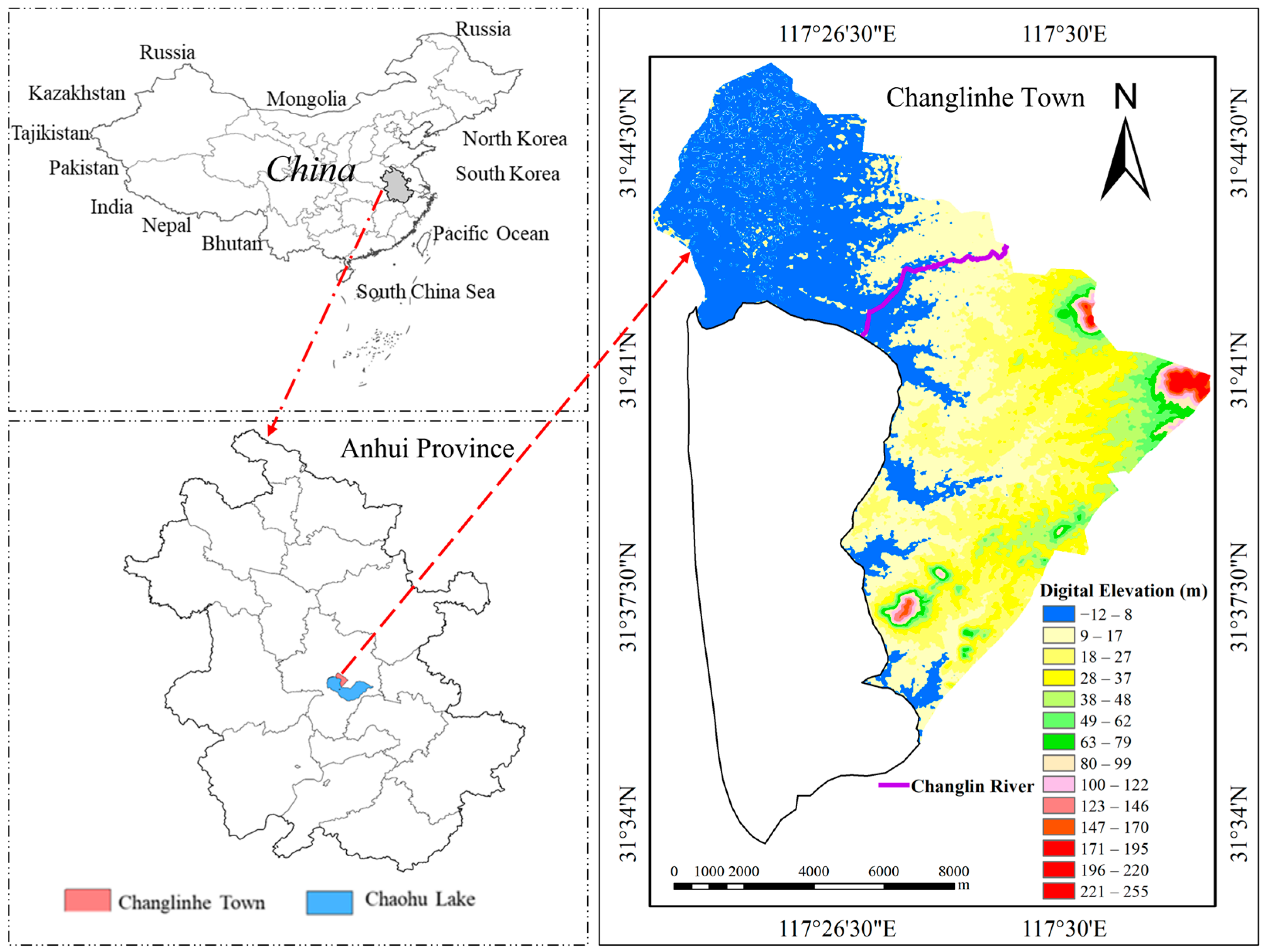
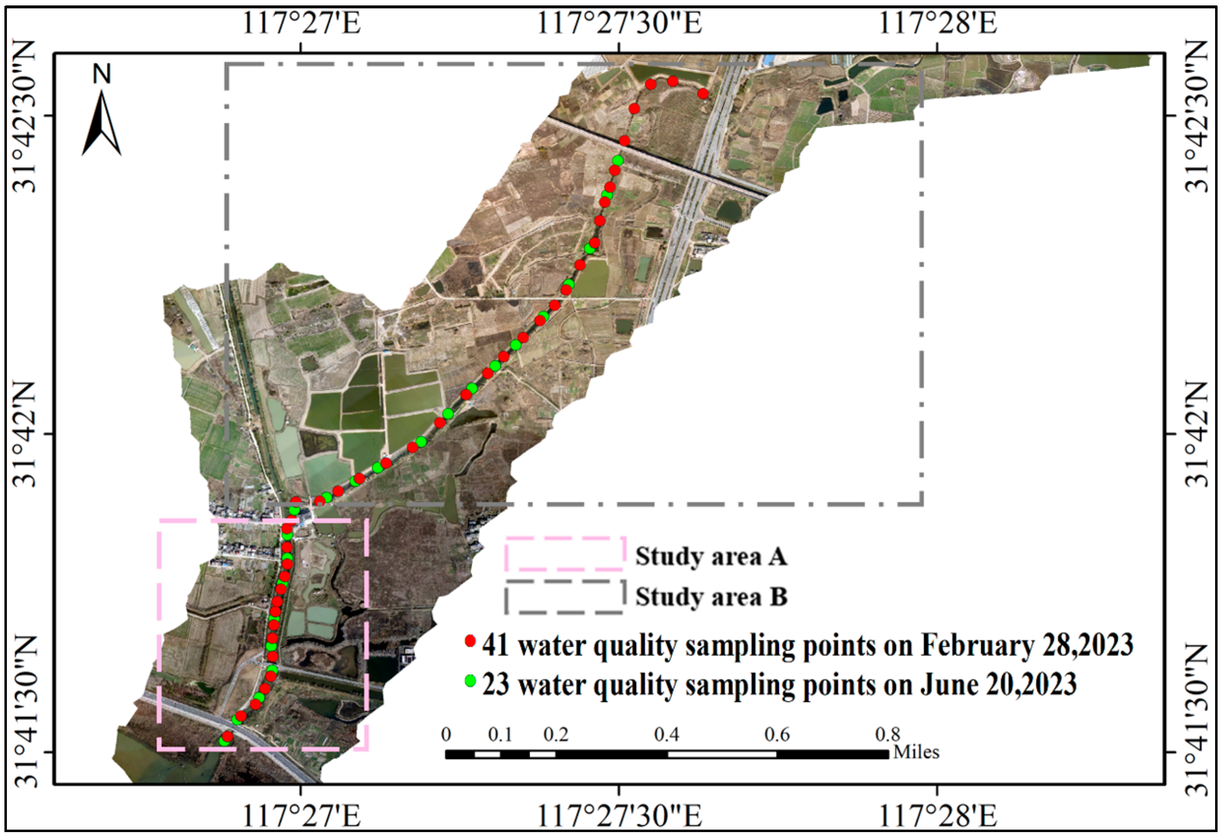
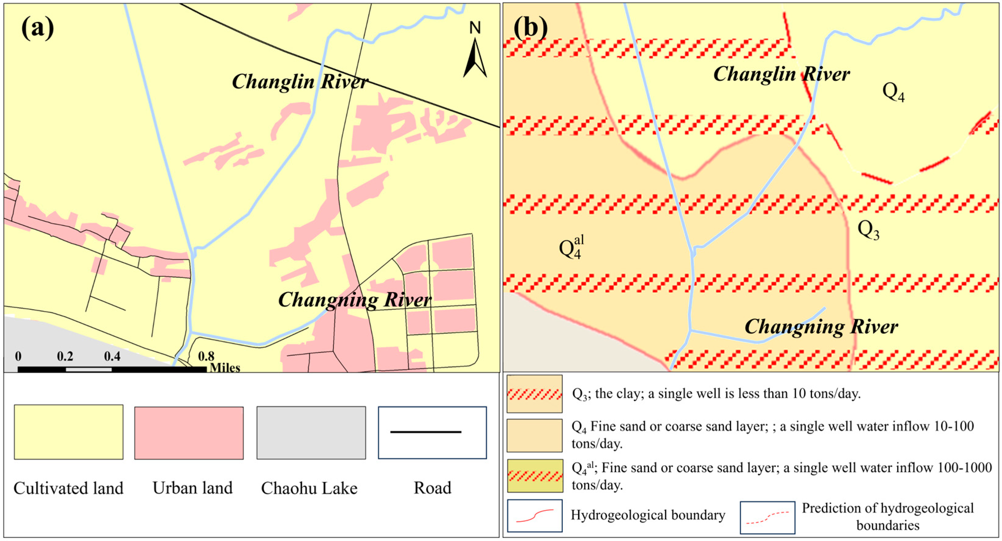
2.1. Study Area

The Changlin River is situated in Feidong County, Hefei City, Anhui Province, Southeast China. It originates from Heihu Mountain and Malong Mountain in Qiaotouji Town, Feidong County, enters into the township of Changlinhe from east to west, and finally flows into the Chaohu Lake (Figure 1). The total length of the Changlin River is about 1.10 × 10⁴ m, and its watershed area is approximately 2.76 × 10⁷ m². The catchment area of the Changlin River belongs to a shallow hillock, and there are large areas of facility agriculture in the middle and upper reaches of the river, with intertwining agricultural production and rural living sources. The Changlin River has heavy pollution loads and a short riparian buffer zone, thus large amounts of pollutants could directly flow into Chaohu Lake. However, the inputs of pollutants (e.g., TN and TP) of the Changlin River to Chaohu Lake have still not been accurately evaluated due to the lack of continuous automatic monitoring data of water quality.

Two representative sections of the Changlin River were selected: Area A and Area B. Area A corresponds to the middle and lower reaches of the Changlin River, and Area B represents the section downstream of the confluence between the Changlin River and the Xinhe River. The detailed location of the study areas and the deployment of sampling points are illustrated in Figure 2. The general investigation procedures are presented in Figure S1, Supporting Information (SI).

2.2. Data Acquisition

2.2.1. UAV Multispectral Images Collection and Processing

A DJI Phantom 4 Multispectral integrated multispectral imaging system (P4M, DJ-Innovations, Shenzhen, China) was used to obtain images of the study area. The multispectral camera comprises six 1/2.9-inch CMOS (Complementary Metal Oxide Semiconductor) sensors, encompassing a single color sensor designed for visible imaging and five monochrome sensors tailored for multispectral imaging. This camera enables the simultaneous acquisition of images in multiple spectral bands, including red (650 ± 16 nm), green (560 ± 16 nm), blue (450 ± 16 nm), near infrared (840 ± 26 nm), and red edge (730 ± 16 nm). The DGI GS Pro can automatically plan flight paths and perform aerial photography tasks based on user-set flight area and camera parameters.

UAV images were obtained on February 28 and 20 June 2023. Notably, the weather on these two days was clear with no or little wind. Firstly, 25%, 50%, and 75% diffuse reflectance standard panels were placed on the ground in the study area, so that the UAV hovered at a certain altitude to take single-band pictures. The complete route task was then automatically planned and completed. The flight altitude was set as 200 m (heading overlap: 60%; side overlap: 70%). Since the UAV flies at a relatively low altitude, no atmospheric correction was required [43].

By using the radiometric calibration page of DJI Terra software (V3.7.6, Shenzhen, China), the calibration plate photos were imported, the calibration plate area was planned, and the calibration plate reflectance coefficients were entered, to achieve the radiometric correction of the multispectral images of the selected area. Then, image stitching was carried out to obtain an orthophoto of the study area with real surface reflectance.

In addition, the latitude and longitude coordinates of the sampling points were imported into ENVI 5.3 software. With the utilization of these coordinates, a region of interest (ROI) measuring 3 × 3 pixels was defined around each sampling site. The average band reflectance within the ROI was then extracted as the final reflectance value for each point.

2.2.2. Manual Monitoring Data

On 28 February and 20 June 2023, 41 and 23 water samples, respectively, were collected at 0.5 m below the water surface using a plexiglass water sampler. The procedures strictly followed the technical guidance specification for sampling of the National Environmental Protection Standard of the People’s Republic of China (HJ 494—2009). One liter of water sample was collected from each sampling site, and the detection of TUB of the collected water samples was obtained via onsite tests by using a turbidimeter (2100Q01-CN, HACH, Shanghai, China). The water samples were quickly transported to the laboratory for storage in a refrigerator under 2–4 °C. A handheld global positioning system (eTrex 229x, Garmin, Taiwan, China) was used throughout the whole sampling process. During sampling, care was taken to avoid places with very narrow channels, shallow water depths, and areas shaded by suspended objects. Attention was also paid to the main river channel, tributaries, and facilities such as agricultural farmland and other incoming water into the mixing place to take water. The determination of TN and TP water quality indicators was completed within 24 h based on HJ 636—2012 (the alkaline potassium persulfate digestion-UV spectrophotometric method) and GB11893-89 (the ammonium molybdate spectrophotometric method) of China, respectively.

2.3. Correlation Analysis and Model Input

Performing band combination operations such as band ratio, addition, subtraction, and normalized index calculation can reduce some background noise, increase the sensitivity of spectral reflectance to water quality parameters, and improve the accuracy of the inversion [41]. Hence, the reflectance of five single bands of red (B1), green (B2), blue (B3), NIR (B4), and red edge (B5) corresponding to the sampling points were first extracted. Then, the following band combinations were used: Bi − Bj, Bi + Bj, Bi/Bj, and (Bi + Bj)/(Bi − Bj) (i and j values can take an integer from 1 to 5, i ≠ j). The results of the band combination calculation were recorded as spectral parameter Vi (Table S1).

Pearson correlation analyses of the 48 spectral parameters were constructed with each water quality indicator. In general, selecting bands or combinations of bands with higher correlation as model inputs can improve the fitting ability and accuracy of a model [26]. The spectral parameters with the highest correlation to the water quality parameters were selected as individual inputs, and the corresponding values of TUB, TN, and TP served as outputs, respectively. The five spectral parameters displaying the highest correlation coefficients with the three metrics (TUB, TN, and TP) were identified as optically sensitive variables. These optically sensitive variables were subsequently used as input features for the subsequent ML modeling. The dataset of 41 water samples collected on 28 February 2023, was divided into a training set (n = 28) and a test set (n = 13) at a ratio of approximately 7:3.

2.4. Machine Learning Models

2.4.1. Ridge Regression (RR)

Ridge Regression, a regularization technique, incorporates a regularization term into least squares regression to address the issue of multicollinearity within regression analysis [44,45]. By striking a balance between model accuracy and generalization across a wider range of samples, it enhances the fitness of the model. The key parameters to be fine-tuned in RR are the regularization strength (λ) and the maximum number of iterations (max iter).

2.4.2. Random Forest (RF) and Grid Search Random Forest (GS-RF)

The basic principle of the RF algorithm is to train multiple CART (Classification and Regression Tree) decision tree weak learners to pack and combine them into one strong learner, and ultimately take the average of the outputs of the multiple weak learners or take a majority vote as the outputs [46,47,48]. RF has two aspects of randomness: (1) there is a sampling procedure on the training set with replacement, which makes the composition of the training set samples random; and (2) each decision tree is modeled by randomly selecting a certain number of features, which gives diversity in the way features are selected for a single decision tree. This makes the RF have strong resistance to overfitting and noises. Therefore, the main parameters to be regulated in the RF regression grid search method are tree (number of decision trees) and max feature (number of features randomly selected per decision tree) [49]. The difference between GS-RF and RF is that RF is realized by manual parameter tuning by the user.

2.4.3. Support Vector Regression (SVR) and Grid Search Support Vector Regression (GS-SVR)

SVR is a regression task that maps linearly indivisible low-dimensional feature data into a high-dimensional space and identifies the optimal hyperplane by a kernel function to minimize the distance between the sample and the hyperplane to build a linear regression [50,51]. In this work, the radial basis kernel function is utilized for support vector regression, and the important parameters C (penalty coefficient) and gamma (coefficient of the kernel function) of the radial basis support vector machine model are adjusted using the grid search method [29].

2.4.4. Extreme Gradient Boosting Regression (XGBoost)

The XGBoost algorithm is an integrated learning method for boosting based on multiple trees [52]. The modeling procedures are as below: a single tree is constructed to make predictions on the training set at first, and then the prediction residuals are fitted iteratively. In this way, n trees are trained, each tree gets a leaf node, and the corresponding scores of each tree are summed up to get the sample prediction value. XGBoost improves prediction ability by reducing the model bias significantly. There are several important parameters during the regression: learning rate, the step size of the iterative decision tree, and the value range (0–1). The smaller the step size is, the slower the training speed is and the easier the model is to overfit. As the value of max depth increases, the more complexly the model will be recorded. The value of gamma ranges from 0 to 1, and the larger the gamma, the more conservative the algorithm [53].

2.4.5. Deep Neural Networks (DNN)

Deep Neural Networks (DNN) represent a deep learning model comprising multiple layers of interconnected neural networks that utilize weighted connections to process and transmit information [34,54]. The Rectified Linear Unit (ReLU) function is chosen as the activation function, introducing nonlinearity to the model. The main parameters regulated are the number of hidden layers, the number of neurons in each hidden layer, and the learning rate. More layers and neurons can improve the expressive enhancement of the model but can also lead to model overfitting. Too large a learning rate may cause the model to oscillate or diverge during training, while too small a learning rate may cause the model to converge slowly.

2.4.6. Convolutional Neural Networks (CNN)

Convolutional Neural Networks (CNN) are a category of feedforward neural networks characterized by their incorporation of convolutional computations and deep structures. The integrated neural network can extract information from input data at a higher level, leveraging its hierarchical structure to obtain profound image details and demonstrating remarkable performance in water quality inversion [14,55]. In this paper, (ReLU) is used as the activation function of each layer and dropout is added to prevent overfitting. The main parameters to be tuned are the number of convolutional layers, the size of the convolutional kernel, the number of convolutional kernels, the number of iterations, and the learning rates.

2.4.7. Catboost Regression (CBR)

CBR is a boost-integrated learning algorithm based on a fully symmetric binary tree-based learner [56]. Prediction bias means that the loss function uses the same dataset to obtain the gradient of the current model, and then trains to obtain the base learner. However, this can lead to biased gradient estimation, which in turn leads to overfitting of the model. The CBR model counters noisy points in the training set with sort boosting, which avoids biased gradient estimation, and thus solves the problem of prediction bias. The main parameters to be adjusted are iterations, learning rate, and depth. The CBR algorithm has a performance of algorithmic accuracy that is excellent for regression problems with multiple input features and noisy sample data, and the model has good robustness and generalization [57].

The degree of fit is compared on the training and test datasets to determine whether overfitting occurs. If the R² on the training set is much higher than the R² on the test set, it is necessary to adjust the relevant parameters that may be an overfitting phenomenon, such as the size of the penalty coefficient C in the SVR, the number of and depth of the trees in the integrated tree model (XG-Boost/RF), and the number of convolutional kernels in the CNN, under the condition of a full understanding of the meaning of the model parameters. The model parameters are adjusted by randomly dividing the training and test sets and modeling them several times to select the model with a good fit. Table S2 represents the optimal hyperparameter values for each model.

2.5. Model Evaluation

The coefficient of determination (R²), the root mean square error (RMSE), the mean absolute error (MAE), the residual prediction deviation (RPD), and the Nash-Sutcliffe efficiency coefficient (NSE) are used to assess the fitness and accuracy of the established models. R² represents the degree of fit of the model, and the closer R² is to 1, the better the model explains the dependent variable. RMSE and MAE are two metrics that quantify the level of disparity between the predicted and actual values. The model’s precision increases as these metrics near zero. RPD is usually used to indicate the reliability of the model. Better predictive performance of the model will be obtained at a higher RPD value. When RPD > 2.0, it indicates that the model is reliable; when 1.4 < RPD < 2.0, it reflects that the model’s predictive performance is ordinary; and when RPD < 1.4, it indicates that the model’s predictive performance is poor. NSE is a statistical index used to evaluate the degree of fit between model simulation results and observation data [58]. This coefficient is used to quantify the prediction accuracy of the model, and its value ranges from negative infinity to 1. The closer the NSE value is to 1, the better the fitting effect is, while the smaller the NSE value is, the worse the fitting effect is.

$$R^2=1-\frac{{\displaystyle {\sum }_{i=1}^n{(\widehat{y}-y_i)}^2}}{{\displaystyle {\sum }_{i=1}^n{(y_i-{\overline{y}}_i)}^2}}$$

(1)

$$MAE=\frac{1}{n}{\displaystyle \sum _1^n|y_i-{\widehat{y}}_i|}$$

(2)

$$RMSE=\sqrt{\frac{{\displaystyle {\sum }_{i=1}^n{(y_i-{\widehat{y}}_i)}^2}}{n}}$$

(3)

$$RPD=\frac{\sqrt{\frac{1}{n}{\displaystyle \sum _{i=1}^n{(y_i-{\widehat{y}}_i)}^2}}}{RMSE}$$

(4)

where $y_i$ indicates measured value, ${\widehat{y}}_i$ indicates predicted value, ${\overline{y}}_i$ indicates the mean of detected values, and n represents the number of samples.

$$\mathit{NSE}=1-\frac{{\displaystyle \sum _{t=1}^T{(y_i^t-{{\widehat{y}}_i}^t)}^2}}{{\displaystyle \sum _{t=1}^T{(y_i^t-{\overline{y}}_i)}^2}}$$

(5)

where $y_i^t$ represents the measured value at a certain time, ${{\widehat{y}}_i}^t$ represents the predicted value at a certain time, and ${\overline{y}}_i$ represents the total average of measured values.

2.6. Model Stability Evaluation

Data segmentation is an important technique in machine learning that helps to validate the stability, generalization, and performance of models. Research has shown that if small changes in input values result in significant alterations in model output, then the model can be deemed unstable and unreliable [59,60]. To evaluate the stability of the established models, a novel arrangement by selecting subsets of the February 2023 dataset was implemented. Specifically, three ratios, 25% (n = 10), 50% (n = 20), and 75% (n = 30), of the 41 collected samples of the training data were utilized while keeping the original test set intact.

2.7. Model Suitability Evaluation

To evaluate whether the established best models possess the applicability to predict the three water environmental indicators at different times in the Changlin River, a new set of data was collected on 20 June 2023. A total of 23 water samples were collected and measured, and corresponding UAV images of the study area were acquired simultaneously. Then, the new data were used to verify the suitability of the model.

3. Results

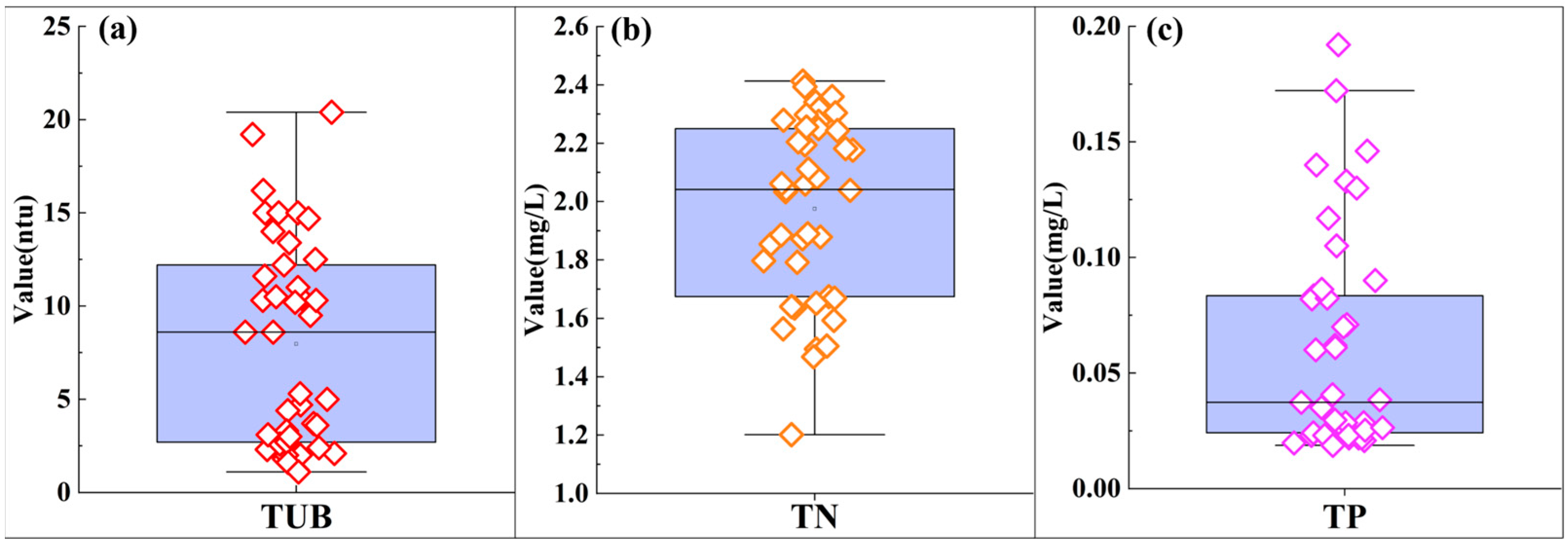
3.1. Water Quality of the Changlin River

The TUB, TN, and TP levels of the 41 water samples collected on 28 February 2023, are shown in Figure 3. The contents of TUB, TN, and TP ranged from 1.10–20.4 ntu (mean value: 7.96 ntu), 1.20–2.41 mg/L (mean value: 1.98 mg/L), and 1.80 × 10⁻²–1.92 × 10⁻¹ mg/L (mean value: 6.10 × 10⁻² mg/L), respectively.

Among 41 water samples, about 56% were lower than the Category V water standard value, about 36.5% were assigned to Category V water, and about 7.5% belonged to Category IV water for TN, based on the limited values stipulated by Environmental Quality Standards for Surface Water of China (GB 3838-2002) (

Table 1. Environmental Quality Standards for Surface Water of China (mg/L).

Water Quality Parameter	I	II	III	IV	V
TN≤	0.2	0.5	1.0	1.5	2.0
TP≤	0.02	0.1	0.2	0.3	0.4

). Meanwhile, about 19% of the water belonged to Category III, and the remaining 81% were Category I or II for TP. Such a result indicated that the major pollution indicator in the study area was TN (Figure 3). When TN accumulates in water over an extended period, it may exacerbate the degradation of the aquatic environment, e.g., by stimulating excessive algae growth and ultimately resulting in eutrophication of the water body [61].

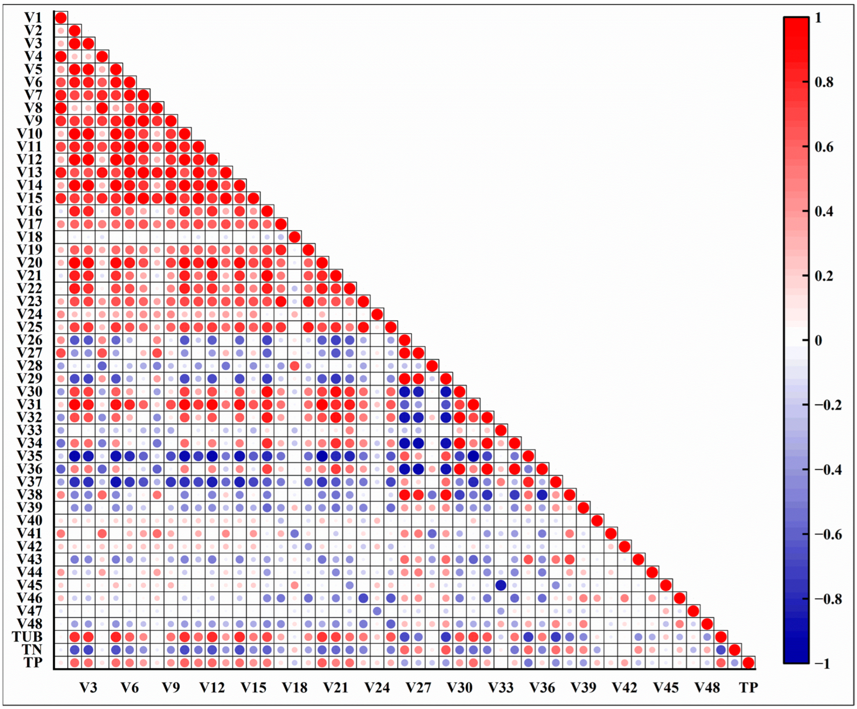
3.2. Correlations between Spectral Parameters and Model Inputs

The spectral profiles of some samples of the preprocessed UAV multispectral images are shown in Figure S2. Strong reflection peaks in the green and near-red spectral ranges demonstrated strong absorption near the red wave. Pearson correlation analyses of the 48 spectral parameters were constructed with each water quality indicator (Figure 4). There was a negative correlation between TN and most of the spectral parameters. While positive correlations between TUB, TP, and most of the spectral parameters were observed, significant correlations were also shown between the spectral parameters.

The five spectral parameters displaying the highest correlation coefficients with the three metrics (TUB, TN, and TP) were identified as optically sensitive variables. These optically sensitive variables were subsequently employed as input features for the ML model. The optically sensitive parameters for TUB were V3 (B3), V5 (B5), V10 (B2 + B3), V12 (B2 + B5), and V14 (B3 + B5), and their Pearson correlation coefficients were ≥0.80. The optically sensitive parameters for TN were V2 (B2), V3 (B3), V10 (B2 + B3), V12 (B2 + B5), and V14 (B3 + B5), with their correlation coefficients ≥0.60. The optically sensitive parameters for TP were V2 (B2), V10 (B2 + B3), V12 (B2 + B5), V16 (B1–B2), and V21 (B2–B4), and their correlation coefficients were ≥0.40. As an optically sensitive parameter, TUB is often able to achieve good correlation results due to its direct influence on water reflectance. The maximum correlation spectral parameters of each water quality parameter are often affected by different water types, water quality parameter concentrations, and water depth. Therefore, the analysis results are somewhat different [62,63].

3.3. Univariate Regression Models

Since it had the highest correlation with TUB and TN according to the correlation analysis, V3 (B3) was selected as an input to establish the univariate model for these two indicators. Similarly, V10 (B2 + B3) was selected as input to build the univariate regression model for TP. The linear, quadratic, and cubic models were constructed separately for each parameter based on Statistics 27 software (

Table 2. Single-variable regression models for three water quality indicators.

Parameter	Index	Modeling Formula	Training Set	Test Set
			R2	R2	RMSE	MAE	RPD
TUB (ntu)	V3	y = −7.2 × 105X3 + 711X − 12.2	0.74	0.79	2.59	1.83	2.19
TN (mg/L)	V3	y = 1410X3 − 28.6X + 2.9	0.55	0.14	0.29	0.24	1.08
TP (mg/L)	V10	y = −34X3 + 16X2 − 1.6X + 0.1	0.52	0.36	0.02	0.02	1.25

and Table S3).

As shown in Table 2, TUB, TN, and TP are well fitted in the univariate cubic regression models. The R² of the three established models for describing TUB, TN, and TP were 0.74, 0.55, and 0.52 in the training set, and 0.79, 0.14, and 0.36 in the test set, respectively. Such results indicated that TUB as a water color parameter could achieve relatively good accuracy in the cubic regression model fitting.

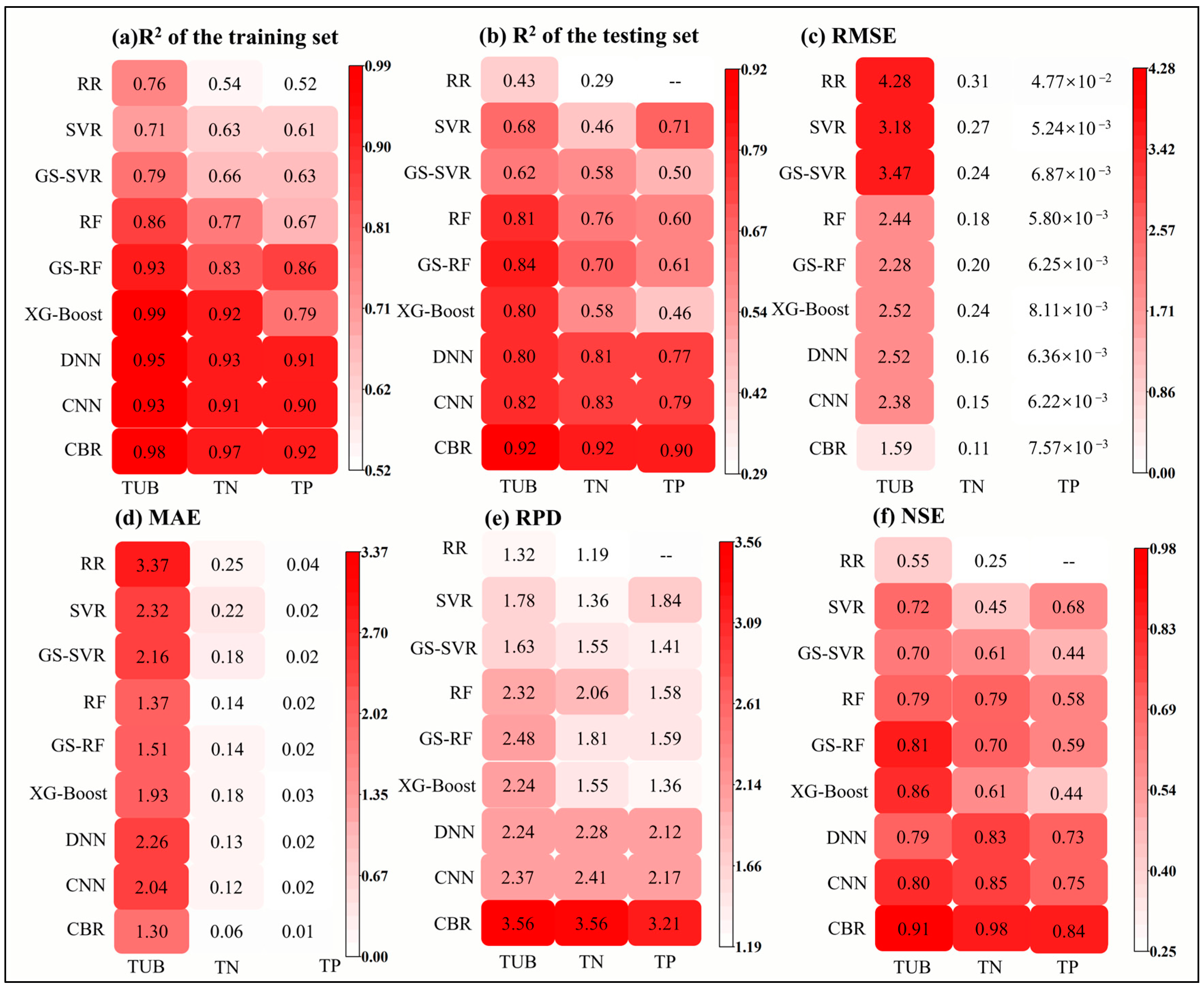
3.4. Fitness of ML Models

Nine different machine models (RR, SVR, GS-SVR, RF, GS-RF, XGBoost, DNN, CNN, and CBR) for TUB, TN, and TP were established independently, and the fitness of these models was evaluated (Figure 5). It was found that the fitness of the nine ML models for TN and TP was better than that of traditional univariate regression methods. This result suggests that indicators with obvious optical activity characteristics, i.e., TUB, can be achieved using simple statistical regression models. Meanwhile, ML algorithms may be more suitable for the quantitative inversion of nonoptically sensitive indicators, e.g., TN and TP [16]. For nonoptical sensitive parameters such as TN and TP, concentrations are typically associated with multiple factors, including chemical composition, biological activity, and so on. These multivariate relationships are better suited for ML algorithms, as they can capture intricate nonlinear associations.

Moreover, CBR was the best model for describing TN, TP, and TUB, with its best performance for TUB (R² = 0.98 of the training set, R² = 0.92, RMSE = 1.59 ntu, MAE = 1.30, RPD = 3.56, NSE = 0.91 of the test set), second for TN (R² = 0.97 of the training set, R² = 0.92, RMSE = 0.11 mg/L, MAE = 0.06, RPD = 3.56, NSE = 0.92 of the test set), and then TP (R² = 0.92 of the training set, R² = 0.90, RMSE = 7.57 × 10⁻³ mg/L, MAE = 0.01, RPD = 3.21, NSE = 0.84 of the test set). The RPD of CBR on the test set for all three metrics (TUB, TN, and TP) was greater than 2.0, indicating that the model was reliable. The residuals between predicted values via CBR models and observed values of TUB, TN, and TP in the test set are presented in Figure 6. Most of the residual values are close to 0, suggesting a better predictive ability of the model. It is noted that the R² values of both CBR and the other eight machine learning algorithms on the training set are greater than those on the test set, indicating overfitting of the model. This is probably due to the presence of noisy data in the sample dataset, which resulted in overlearning of the ML model about individual features of the dataset rather than essential patterns [64].

3.5. Optimal Model Validation

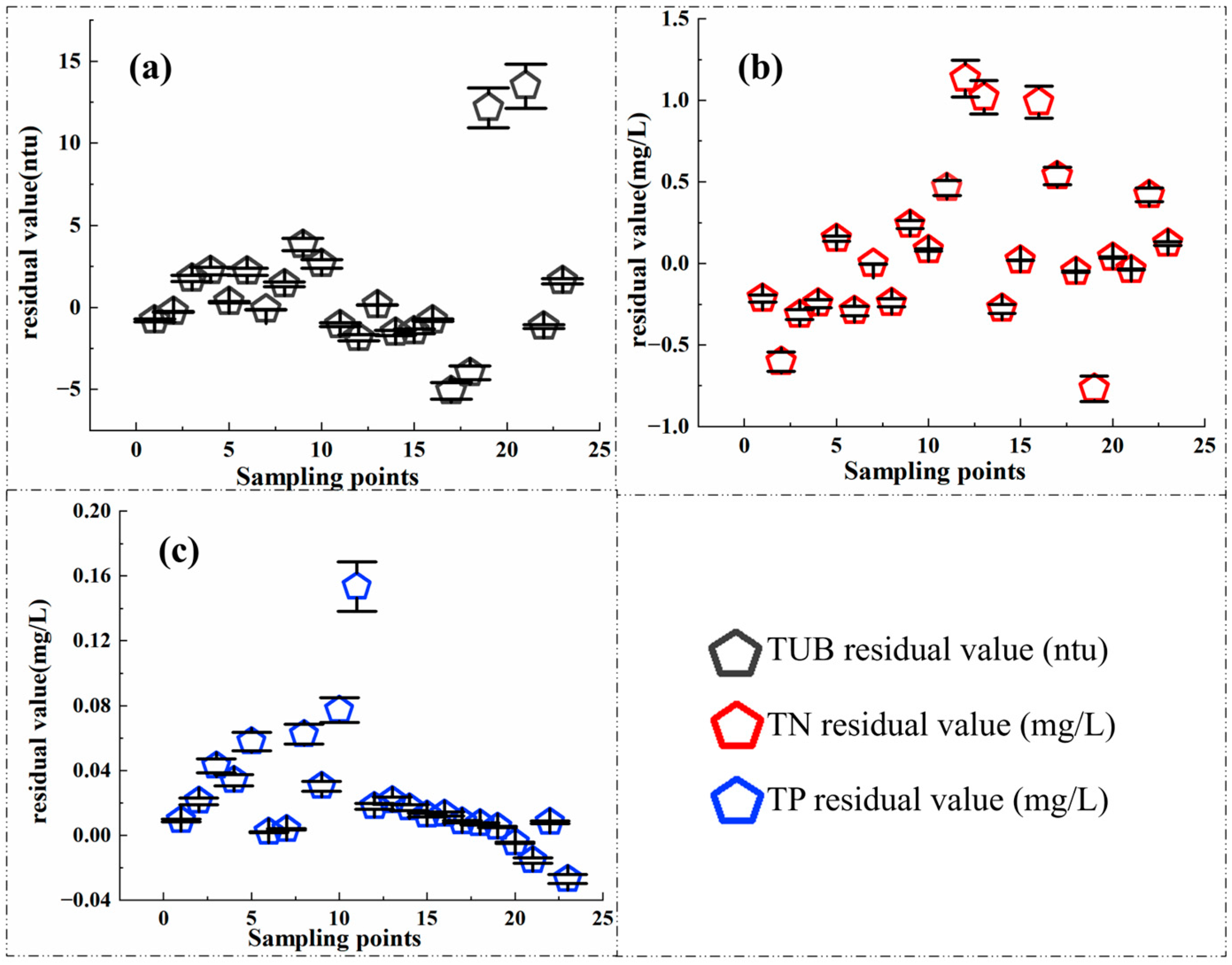
3.5.1. Stability of the ML Models

It was found that the CBR model fits TUB, TN, and TP poorly when only 25% of the samples are available, and the overall coefficient of determination (R²) tends to increase gradually with the incremental increase of the sample size (Figure 7 and

Table 3. The model stability evaluation indexes under different sample sizes.

Sample Size	Evaluation Index	TUB	TN	TP
25%	R2	0.70	0.43	0.49
	RMSE	4.68	0.06	0.03
	MAE	1.67	0.19	0.01
	RPD	1.82	1.33	1.41
50%	R2	0.72	0.61	0.65
	RMSE	4.29	0.04	0.02
	MAE	1.68	0.16	0.01
	RPD	1.90	1.61	1.68
75%	R2	0.77	0.71	0.74
	RMSE	3.52	0.03	0.02
	MAE	1.53	0.14	0.01
	RPD	2.09	1.86	1.96

). When the sample size is reduced to 75%, the model’s predictive accuracy declines compared with the accuracy achieved when using the entire dataset for training. This phenomenon is likely attributed to shifts in sample diversity as the sample size decreases, resulting in what is known as prediction bias [36].

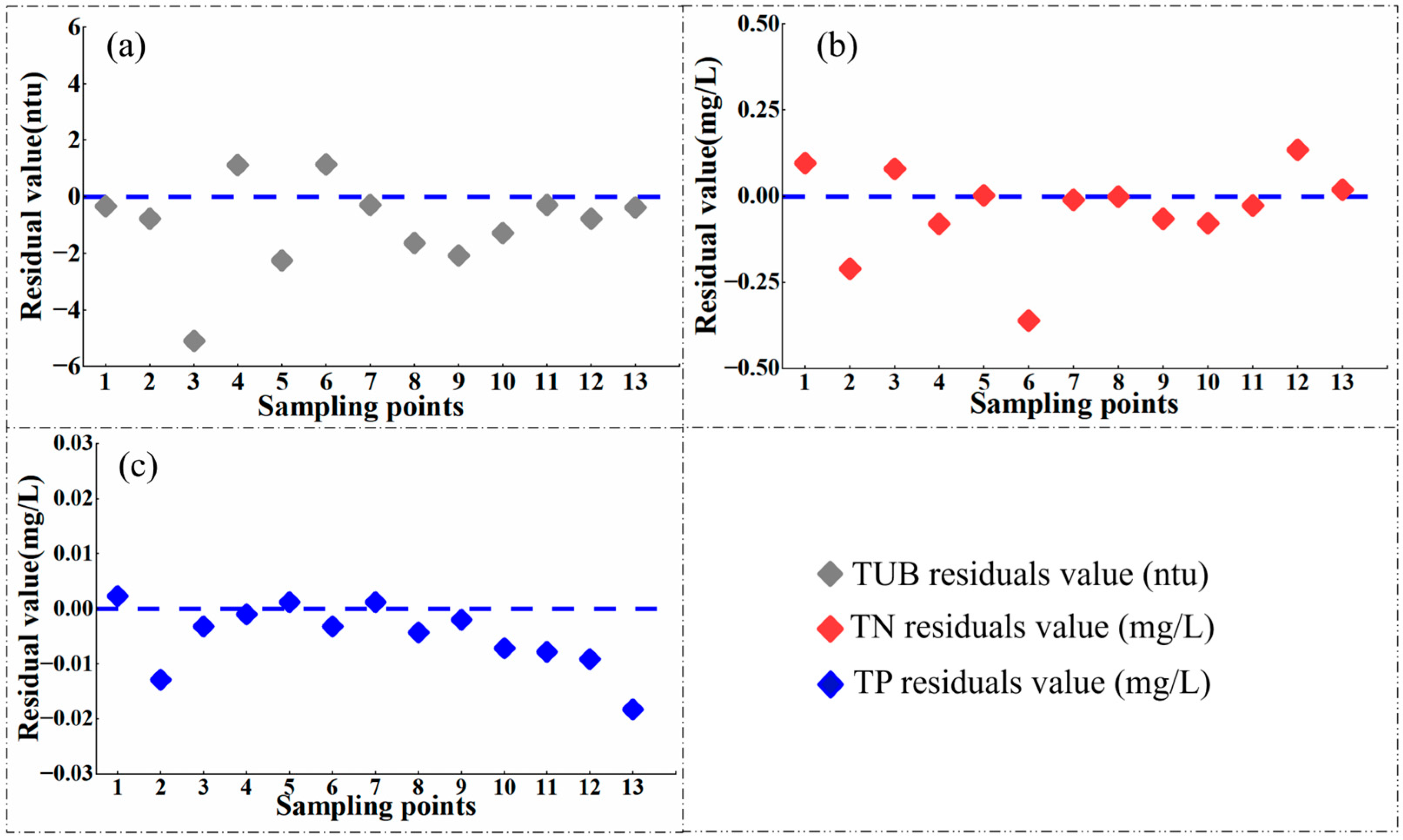
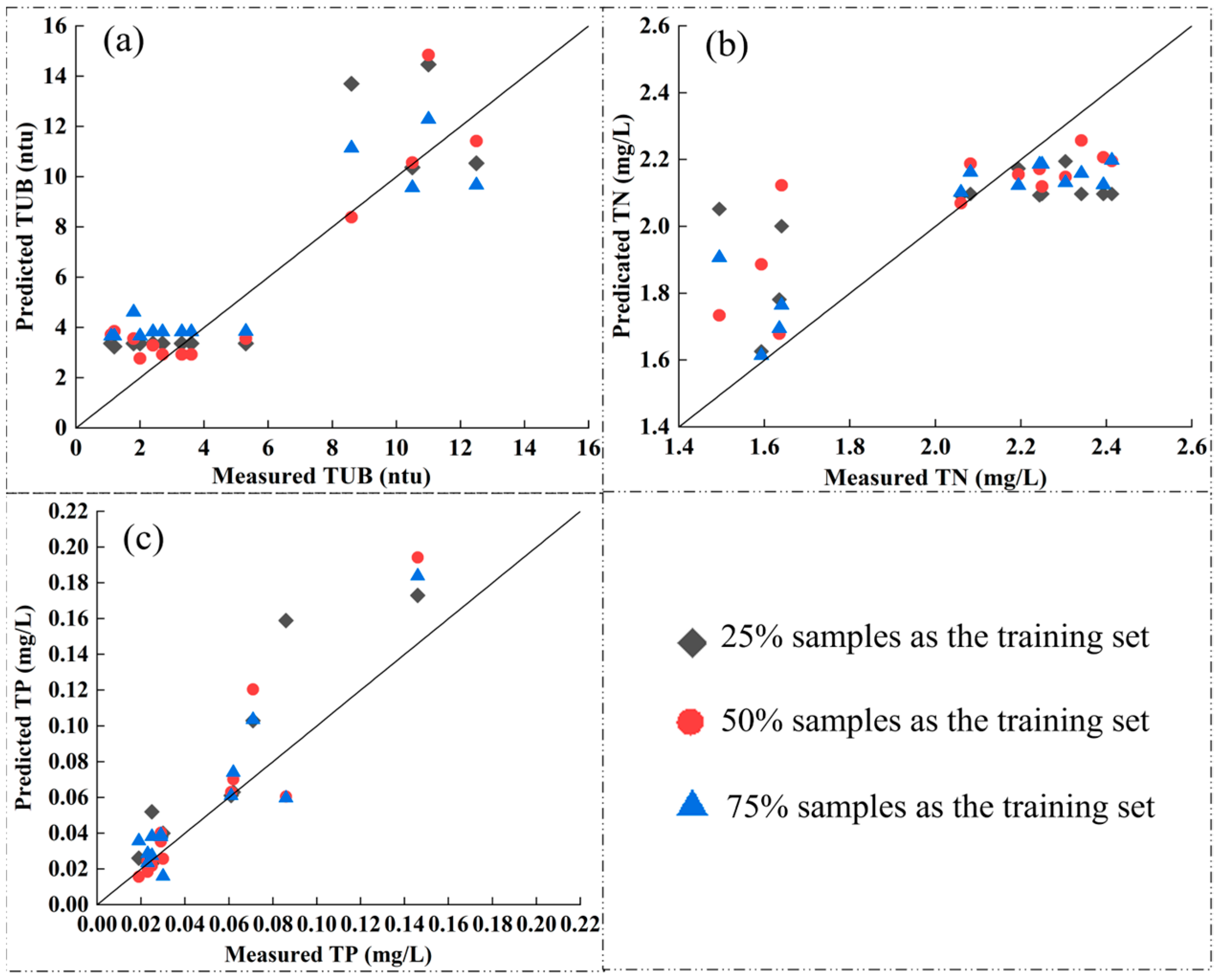
3.5.2. Verification of Model Suitability

The results show that the model had certain applicability at different sample times, and there were also deviations between the predicted values and true values of TN and TUB at several sample sites (Figure 8).

Overall, the values of the three indicators in the dataset obtained in June 2023 were higher than those in the dataset obtained in February. The training set of the CBR model contained little high values, which, to some extent, led to the underestimation of high values in the test set. This phenomenon is possibly due to the large gap in the distribution of indicator values in the training set and the test set, and the sample imbalance in the training set might not cover the whole sample space well [16].

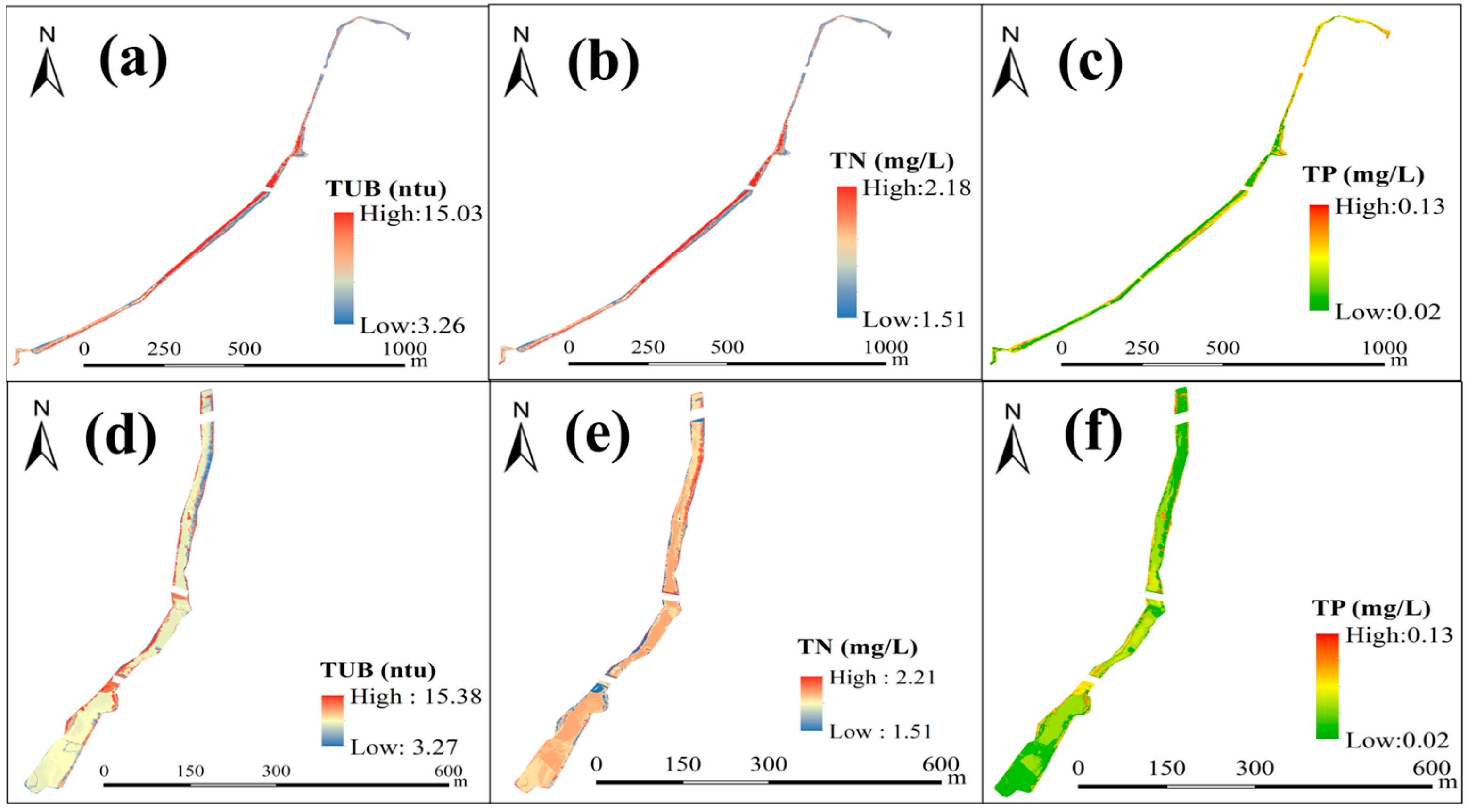
3.6. Spatial Distribution Characteristics of Water Quality Parameters

Firstly, the fusion of five single-band images of the study area was carried out in ENVI 5.3 software using the Layer Stacking module. Based on this, the UAV images of the study area of the river were extracted by using a mask in the visual interpretation method in ENVI 5.3 software. Then, the CBR model and related parameters were saved, and the UAV multispectral images of the river extracted by the mask were inputted to finally obtain the inversion results of each water quality parameter (Figure 9).

The inversion results showed that TUB, TN, and TP were in the ranges of 3.26–15.38 ntu, 1.51–2.21 mg/L, and 0.02–0.13 mg/L, respectively. Based on TN values, the water quality of the Changlin River was Class V and even worse. Meanwhile, based on the TP inversion results, none of the levels exceeded the Class III standard. Thus, the overall water quality in the study area was between Class V and inferior Class V (GB 3838-2002 of China), basically consistent with the actual measured results listed in Section 3.1.

The distribution map of TN and TP concentrations indicates that the colors along the riverbanks are more vibrant than in the central section (Figure 9). This phenomenon is likely attributed to the presence of pollution sources along the riverbanks. As can be seen from Figure 9, the TN pollution in Area B was more severe than that in Area A in general. Area A is a section of the river where two tributaries, the New River and Changning River, converge one after another, and is close to Chaohu Lake. Field investigations suggested that there were no obvious drainage outlets of pollutants on either side of this section, but wastewater generated by the township sewage treatment plants may have been discharged into the river and converged into this section via surface runoff. Hence, it was speculated that the main source of pollutants in this section of the river might be drainage from sewage treatment plants. There are highly concentrated agricultural planting areas and fishpond breeding areas located around Area B, and onsite field investigations found that there are fishpond drainage culverts on both sides of the riverbanks. Several obvious farmland drainage outlets also were found.

3.7. Land-Use Characteristics of the Study Area

Land-use types can influence human production activities and the distribution of pollutants in rivers to a large extent [65]. In general, watershed nitrogen and phosphorus levels are positively correlated with the proportion of agricultural and residential land uses [66,67]. Based on the land-use map (Figure 10a), the area around study areas A and B is generally agricultural land. Through in-depth household surveys conducted in the 11 communities under the jurisdiction of the Changlin River, it was found that the application of fertilizer on farmland is inefficient. Crops often transport unabsorbed nutrients such as nitrogen and phosphorus, along with a certain proportion of applied fertilizers, into rivers via surface runoff and groundwater flow, resulting in adverse impacts on water quality. Analysis of the hydrogeological map (Figure 10b) indicates that the Q₃ region has relatively low soil permeability, making it difficult for pollutants to infiltrate into the groundwater. The Q₄ and Q₄^al areas, on the other hand, exhibit higher soil permeability, facilitating a relatively easier infiltration of pollutants.

According to information provided by the Agricultural and Rural Department of Fei-dong County, the intensity of fertilizer application in Changlinhe Township in 2021 was up to 6.25 × 10⁻² kg/m², which is 2.8-fold the safe level of fertilizer application stipulated by developed countries (2.25 × 10⁻² kg/m²) [68]. Therefore, unreasonable fertilizer application and overfertilization in pursuit of yield are important reasons for the deterioration of the water environment quality in the Changlin River.

According to field investigation results, the water of the Changlin River is mainly used for agricultural irrigation rather than for daily drinking water supply. Given that the Changlin River flows into Chaohu Lake (one of the five major freshwater lakes in China), the local environmental authorities must strengthen their oversight. Strictly regulation of the usage of pesticides and chemical fertilizers by residents and, concurrently, promoting the application of organic fertilizers is required. In addition, the potential introduction of floating bed plant technology should be considered as a means for reducing the presence of pollutants in the river.

4. Discussion

4.1. Model Performance Analysis

For the TUB index, among the nine machine algorithms, the three worst-performing algorithms were RR, SVR, and GS-SVR, and the R² of the test set was below 0.68. This may be because SVR is very sensitive to parameter selection, and GS-SVR may not be able to explore the entire search space and may miss important areas [69,70]. Attention should be drawn to the fact that RR exhibits R² below 0.50 for all three indicators in the test set, indicating notable prediction error. This limitation may stem from the fact that RR relies on the assumptions of linear models, rendering it less adept at capturing the intricacies of complex nonlinear relationships [71]. Upon comparing the fitting effects of the TN and TP indicators, the top three algorithms were DNN, CNN, and CBR, all achieving an R² exceeding 0.77 on the test set. This may be attributed to the sensitivity of DNN and CNN to underlying connections in the dataset, allowing them to adjust weight parameters in reverse to bring predicted values closer to actual values, thereby exhibiting a strong fitting performance. However, during the training process, it was observed that increasing the number of hidden layers did not lead to a significant increase in the coefficient of determination, R². This could be because deep learning algorithms typically require a substantial amount of training data, and the limited dataset in this study restricted the model’s fitting performance to some extent [54,72].

For TUB indicators, the R² accuracy of the test set decreased by 53.75%, 25.82%, 32.46%, 11.67%, 9.12%, 13.09%, 13.00%, and 10.78%, respectively, for the other eight models (RR, SVR, GS-SVR, RF, GS-RF, XGBoost, DNN, CNN) compared with CBR. For the TN, the R² of the test set decreased by 68.02%, 49.47%, 36.25%, 16.32%, 23.81%, 36.13%, 11.44%, and 9.23%, respectively. For the TP index, the R² on the RR model test set was less than 0, and the fitting effect of CBR on TP was much better than that of RR. The coefficients of determination of the other seven models (SVR, GS-SVR, RF, GS-RF, XGBoost, DNN, CNN) compared with the CBR model in the test set decreased by 21.81%, 44.89%, 33.42%, 32.88%, 48.95%, 13.95%, and 12.82%, respectively. CBR has high R², RPD, and NSE, along with low RMSE and MAE in the fitting of the three indicator inversion models, showing good application potential. CBR utilizes adaptive learning rates, which can dynamically fine-tune the learning rate throughout the training process to enhance its alignment with the data’s unique characteristics. Such capability serves to mitigate gradient bias problems during training while upholding the model’s ability to generalize effectively [73].

4.2. Comparison of Inversion Accuracy with Other Research

In an example of studies focusing on small and medium rivers, Zhu et al. [74] successfully inverted the permanganate index (CODMn), N-NH₃ (ammonia nitrogen), and TN in the intricate river network of Qidong (with rivers mostly ranging from 15 to 20 m in width) using Gaofen-1 satellite imagery. The inversion accuracy, represented by R², slightly exceeded 0.5. In a study by Huangfu et al. [75], the inversion of several small/medium-sized rivers (with a minimum width of 10 m) in the Xinyang section of the Huaihe River was achieved based on Sentinel-2 satellite images, yielding R² values ranging from 0.60 to 0.67. Yan et al. [76] successfully inverted dissolved oxygen (DO) and TUB in the Biyu River (with a water area of 10⁵ m² and a length of 2.5 × 10³ m) using UAV multispectral imagery and XGBoost and RF models, with inversion accuracies (R²) ranging from 0.75 to 0.81. Hou et al. [16] conducted a study around the Fuyang River section (with a water area covering about 1.5 × 10⁵ m² and a length of 700 m), achieving the inversion of six water quality indicators based on UAV images and employing partial least squares (PLS), RF, and Lasso models, with R² reaching up to 0.90. In the current study, the inversion of TN, TP, and TUB in the Changlin River (with a water area of 2.76 × 10⁷ m² and a length of 1.10 × 10⁴ m) was realized using the CBR model, and the R² values ranged from 0.90 to 0.92. Compared with satellite imagery, UAV imagery has a high spatial resolution and smaller pixel size, which greatly attenuates the influence of mixed pixels. Due to this characteristic, the error between the actual reflectance of the water at the sampling point and the reflectance of the corresponding pixel is significantly reduced [30]. To sum up, these results show the advantages of high-resolution UAV multispectral imagery in the field of water quality inversion for small/medium-sized rivers.

4.3. Implications of This Study

Low-altitude remote sensing technology is still in its early stage in the field of water quality inversion in small/medium-sized rural rivers, and there is an urgent need to explore more machine learning methods with potential applications. In this study, we validated the predictive performance of the CBR machine learning model in predicting water color parameters (TUB) and nonwater color parameters (TN/TP) and conducted model stability and applicability tests. Our model demonstrated higher reliability and generality relative to those studies focusing on the inversion of a single water quality parameter. This study provides technical support for remote sensing for monitoring of water quality parameters in typical small rural water bodies in the Chaohu Lake Basin, as well as demonstrates the potential application of combining low-altitude remote sensing technology and machine learning algorithms in the field of water quality in small rural water bodies with limited measured data. The superior performance of the CBR model establishes a dependable scientific foundation for water quality monitoring and management. It holds promising potential to play a constructive role in future research and practical applications within the field of water quality monitoring. By using high-resolution multispectral images from UAVs and limited ground monitoring data, remote sensing dynamic monitoring in the study area can be achieved to gain insights into pollution trends and thus formulate effective water pollution prevention and control strategies.

4.4. Limitations and Perspective

Firstly, although the CBR model was well applied in the field of water quality monitoring of medium-/small-sized rural water bodies in the current work, the applicability of the model over time and in different regions needs to be evaluated. The water quality inversion model is more likely to achieve much better accuracy because the individual water quality parameters may exhibit specific spectral characteristics for a fixed area within a fixed period with a relatively fixed source of effluent [74]. The development of a water quality inversion model for the study area in seasons and sub-basins and the applicability of the model in different years over a larger period should be conducted. Secondly, more data are needed to be collected to obtain models for the inversions of other water quality parameters, e.g., DOM (colored dissolved organic matter) and N-NH₃, plankton biomass. Thirdly, we will look for datasets with large standard deviation changes to reveal the effect of training set standard deviation changes on the predictive ability of the model. In addition, Zhu et al. [77] obtained impressive results by employing a transfer learning model to predict DO in Lake Taihu. Chen et al. [78], utilizing a BPNN model, successfully predicted the total suspended solids concentration in Poyang Lake with an R² of 0.89, demonstrating excellent transferability. Future studies could delve deeper into the potential applications of deep learning techniques and transferable machine learning algorithms in the field of water quality monitoring, aiming to further enhance the performance and applicability of monitoring models [79,80,81,82]. Finally, we are considering applying the hyperspectral camera carried by the UAV to the water quality inversion in our subsequent work, to acquire more spectral information, capture finer spectral details, and more accurately obtain the intrinsic optical properties of different components of the water body [83].

5. Conclusions

In summary, based on the UAV images and ground monitoring data of a typical small-sized water body (the Changlin River), the inversion models using nine ML algorithms (i.e., RR, SVR, GS-SVR, RF, GS-RF, XGBoost, DNN, CNN, and CBR) and three univariate regression models (i.e., linear, quadratic, and cubic) for TUB, TN, and TP were established and their inversion performances were compared. The major finds are: (1) significant differences between the algorithms suitable for optical-sensitive parameters and nonoptical-sensitive parameter inversion; (2) the water color parameter TUB can be effectively inverted by a simple univariate regression model, and ML models are more suitable for the inversion of the TN and TP water quality parameters; (3) the CBR model exhibits reliable predictive performance on evaluation metrics, with a test set R² greater than 0.90; (4) based on the examination of diverse sample sizes within the training set and the assessment of the model’s applicability across varying time intervals, the CBR model demonstrates a certain degree of stability and adaptability, showcasing promising application potential; and (5) regional water pollution is significantly related to land-use type, excessive and unreasonable fertilizer application, and the distribution of discharge outlets.

References

1. Hu, W.; Liu, J.; Wang, H.; Miao, D.; Shao, D.; Gu, W. Retrieval of TP Concentration from UAV Multispectral Images Using IOA-ML Models in Small Inland Waterbodies. Remote Sens. 2023, 15, 1250. [Google Scholar] [CrossRef]
2. Sayers, M.J.; Bosse, K.R.; Shuchman, R.A.; Ruberg, S.A.; Fahnenstiel, G.L.; Leshkevich, G.A.; Stuart, D.G.; Johengen, T.H.; Burtner, A.M.; Palladino, D. Spatial and Temporal Variability of Inherent and Apparent Optical Properties in Western Lake Erie: Implications for Water Quality Remote Sensing. J. Great Lakes Res. 2019, 45, 490–507. [Google Scholar] [CrossRef]
3. Brando, V.E.; Dekker, A.G. Satellite Hyperspectral Remote Sensing for Estimating Estuarine and Coastal Water Quality. IEEE Trans. Geosci. Remote Sens. 2003, 41, 1378–1387. [Google Scholar]
4. Alparslan, E.; Aydöner, C.; Tufekci, V.; Tüfekci, H. Water Quality Assessment at Ömerli Dam Using Remote Sensing Techniques. Environ. Monit Assess 2007, 135, 391–398. [Google Scholar] [CrossRef] [PubMed]
5. Tong, X.; Xie, H.; Qiu, Y.; Zhang, H.; Song, L.; Zhang, Y.; Zhao, J. Quantitative Monitoring of Inland Water Using Remote Sensing of the Upper Reaches of the Huangpu River, China. Int. J. Remote Sens. 2010, 31, 2471–2492. [Google Scholar] [CrossRef]
6. Dlamini, S.; Nhapi, I.; Gumindoga, W.; Nhiwatiwa, T.; Dube, T. Assessing the Feasibility of Integrating Remote Sensing and In-Situ Measurements in Monitoring Water Quality Status of Lake Chivero, Zimbabwe. Phys. Chem. Earth Parts A/B/C 2016, 93, 2–11. [Google Scholar] [CrossRef]
7. Smith, V.H.; Tilman, G.D.; Nekola, J.C. Eutrophication: Impacts of Excess Nutrient Inputs on Freshwater, Marine, and Terrestrial Ecosystems. Environ. Pollut. 1999, 100, 179–196. [Google Scholar] [CrossRef]
8. Odermatt, D.; Gitelson, A.; Brando, V.E.; Schaepman, M. Review of Constituent Retrieval in Optically Deep and Complex Waters from Satellite Imagery. Remote Sens. Environ. 2012, 118, 116–126. [Google Scholar] [CrossRef]
9. Sagan, V.; Peterson, K.T.; Maimaitijiang, M.; Sidike, P.; Sloan, J.; Greeling, B.A.; Maalouf, S.; Adams, C. Monitoring Inland Water Quality Using Remote Sensing: Potential and Limitations of Spectral Indices, Bio-Optical Simulations, Machine Learning, and Cloud Computing. Earth-Sci. Rev. 2020, 205, 103187. [Google Scholar] [CrossRef]
10. Virdis, S.G.P.; Xue, W.; Winijkul, E.; Nitivattananon, V.; Punpukdee, P. Remote Sensing of Tropical Riverine Water Quality Using Sentinel-2 MSI and Field Observations. Ecol. Indic. 2022, 144, 109472. [Google Scholar] [CrossRef]
11. Lu, H.; Ma, X. Hybrid Decision Tree-Based Machine Learning Models for Short-Term Water Quality Prediction. Chemosphere 2020, 249, 126169. [Google Scholar] [CrossRef]
12. Cortes, C.; Vapnik, V. Support-Vector Networks. Mach. Learn. 1995, 20, 273–297. [Google Scholar] [CrossRef]
13. Zhou, Y.; He, B.; Xiao, F.; Feng, Q.; Kou, J.; Liu, H. Retrieving the Lake Trophic Level Index with Landsat-8 Image by Atmospheric Parameter and RBF: A Case Study of Lakes in Wuhan, China. Remote Sens. 2019, 11, 457. [Google Scholar] [CrossRef]
14. Pyo, J.; Park, L.J.; Pachepsky, Y.; Baek, S.-S.; Kim, K.; Cho, K.H. Using Convolutional Neural Network for Predicting Cyanobacteria Concentrations in River Water. Water Res. 2020, 186, 116349. [Google Scholar] [CrossRef]
15. He, Y.; Gong, Z.; Zheng, Y.; Zhang, Y. Inland Reservoir Water Quality Inversion and Eutrophication Evaluation Using BP Neural Network and Remote Sensing Imagery: A Case Study of Dashahe Reservoir. Water 2021, 13, 2844. [Google Scholar] [CrossRef]
16. Hou, Y.; Zhang, A.; Lv, R.; Zhang, Y.; Ma, J.; Li, T. Machine Learning Algorithm Inversion Experiment and Pollution Analysis of Water Quality Parameters in Urban Small and Medium-Sized Rivers Based on UAV Multispectral Data. Environ. Sci Pollut Res 2023, 30, 78913–78932. [Google Scholar] [CrossRef] [PubMed]
17. Huo, A.; Zhang, J.; Qiao, C.; Li, C.; Xie, J.; Wang, J.; Zhang, X. Multispectral Remote Sensing Inversion for City Landscape Water Eutrophication Based on Genetic Algorithm-Support Vector Machine. Water Qual. Res. J. 2014, 49, 285–293. [Google Scholar] [CrossRef]
18. Shen, L.Q.; Amatulli, G.; Sethi, T.; Raymond, P.; Domisch, S. Estimating Nitrogen and Phosphorus Concentrations in Streams and Rivers, within a Machine Learning Framework. Sci. Data 2020, 7, 161. [Google Scholar] [CrossRef] [PubMed]
19. Li, X.; Huang, M.; Wang, R. Numerical Simulation of Donghu Lake Hydrodynamics and Water Quality Based on Remote Sensing and MIKE 21. Int. J. Geo-Inf. 2020, 9, 94. [Google Scholar] [CrossRef]
20. Tan, Z.; Ren, J.; Li, S.; Li, W.; Zhang, R.; Sun, T. Inversion of Nutrient Concentrations Using Machine Learning and Influencing Factors in Minjiang River. Water 2023, 15, 1398. [Google Scholar] [CrossRef]
21. Xiaojuan, L.; Mutao, H.; Jianbao, L. Remote Sensing Inversion of Lake Water Quality Parameters Based on Ensemble Modelling. E3S Web Conf. 2020, 143, 02007. [Google Scholar] [CrossRef]
22. Wang, L.; Yue, X.; Wang, H.; Ling, K.; Liu, Y.; Wang, J.; Hong, J.; Pen, W.; Song, H. Dynamic Inversion of Inland Aquaculture Water Quality Based on UAVs-WSN Spectral Analysis. Remote Sens. 2020, 12, 402. [Google Scholar] [CrossRef]
23. Sharafati, A.; Asadollah, S.B.H.S.; Hosseinzadeh, M. The Potential of New Ensemble Machine Learning Models for Effluent Quality Parameters Prediction and Related Uncertainty. Process Saf. Environ. Prot. 2020, 140, 68–78. [Google Scholar] [CrossRef]
24. Xiao, Y.; Guo, Y.; Yin, G.; Zhang, X.; Shi, Y.; Hao, F.; Fu, Y. UAV Multispectral Image-Based Urban River Water Quality Monitoring Using Stacked Ensemble Machine Learning Algorithms—A Case Study of the Zhanghe River, China. Remote Sens. 2022, 14, 3272. [Google Scholar] [CrossRef]
25. Li, S.; Song, K.; Wang, S.; Liu, G.; Wen, Z.; Shang, Y.; Lyu, L.; Chen, F.; Xu, S.; Tao, H.; et al. Quantification of Chlorophyll-a in Typical Lakes across China Using Sentinel-2 MSI Imagery with Machine Learning Algorithm. Sci. Total Environ. 2021, 778, 146271. [Google Scholar] [CrossRef] [PubMed]
26. Tran, M.D.; Vantrepotte, V.; Loisel, H.; Oliveira, E.N.; Tran, K.T.; Jorge, D.; Mériaux, X.; Paranhos, R. Band Ratios Combination for Estimating Chlorophyll-a from Sentinel-2 and Sentinel-3 in Coastal Waters. Remote Sens. 2023, 15, 1653. [Google Scholar] [CrossRef]
27. Yang, H.; Kong, J.; Hu, H.; Du, Y.; Gao, M.; Chen, F. A Review of Remote Sensing for Water Quality Retrieval: Progress and Challenges. Remote Sens. 2022, 14, 1770. [Google Scholar] [CrossRef]
28. Shi, K.; Wang, P.; Yin, H.; Lang, Q.; Wang, H.; Chen, G. Dissolved Oxygen Inversion Based on Himawari-8 Imagery and Machine Learning: A Case Study of Lake Chaohu. Water 2023, 15, 3081. [Google Scholar] [CrossRef]
29. Li, Y.; He, L.; Peng, B.; Fan, K.; Tong, L. Remote Sensing Inversion of Water Quality Parameters in Longquan Lake Based on PSO-SVR Algorithm. In Proceedings of the IGARSS 2018—2018 IEEE International Geoscience and Remote Sensing Symposium, Valencia, Spain, 22–27 July 2018; pp. 9268–9271. [Google Scholar]
30. Fu, B.; Lao, Z.; Liang, Y.; Sun, J.; He, X.; Deng, T.; He, W.; Fan, D.; Gao, E.; Hou, Q. Evaluating Optically and Non-Optically Active Water Quality and Its Response Relationship to Hydro-Meteorology Using Multi-Source Data in Poyang Lake, China. Ecol. Indic. 2022, 145, 109675. [Google Scholar] [CrossRef]
31. Wang, X.; Zhang, F.; Ding, J. Evaluation of Water Quality Based on a Machine Learning Algorithm and Water Quality Index for the Ebinur Lake Watershed, China. Sci. Rep. 2017, 7, 12858. [Google Scholar] [CrossRef]
32. Cao, X.; Zhang, J.; Meng, H.; Lai, Y.; Xu, M. Remote Sensing Inversion of Water Quality Parameters in the Yellow River Delta. Ecol. Indic. 2023, 155, 110914. [Google Scholar] [CrossRef]
33. Ding, H.; Li, R.R.; Lin, H.; Wang, X. Monitoring and Evaluation on Water Quality of Hun River Based on Landsat Satellite Data. In Proceedings of the 2016 Progress in Electromagnetic Research Symposium (PIERS), Shanghai, China, 8–11 August 2016; IEEE: Shanghai, China, 2016; pp. 1532–1537. [Google Scholar]
34. Qian, J.; Liu, H.; Qian, L.; Bauer, J.; Xue, X.; Yu, G.; He, Q.; Zhou, Q.; Bi, Y.; Norra, S. Water Quality Monitoring and Assessment Based on Cruise Monitoring, Remote Sensing, and Deep Learning: A Case Study of Qingcaosha Reservoir. Front. Environ. Sci. 2022, 10, 979133. [Google Scholar] [CrossRef]
35. Qun’ou, J.; Lidan, X.; Siyang, S.; Meilin, W.; Huijie, X. Retrieval Model for Total Nitrogen Concentration Based on UAV Hyper Spectral Remote Sensing Data and Machine Learning Algorithms—A Case Study in the Miyun Reservoir, China. Ecol. Indic. 2021, 124, 107356. [Google Scholar] [CrossRef]
36. Chen, B.; Mu, X.; Chen, P.; Wang, B.; Choi, J.; Park, H.; Xu, S.; Wu, Y.; Yang, H. Machine Learning-Based Inversion of Water Quality Parameters in Typical Reach of the Urban River by UAV Multispectral Data. Ecol. Indic. 2021, 133, 108434. [Google Scholar] [CrossRef]
37. Li, Y.; Li, S.; Song, K.; Liu, G.; Wen, Z.; Fang, C.; Shang, Y.; Lyu, L.; Zhang, L. Sentinel-3 OLCI Observations of Chinese Lake Turbidity Using Machine Learning Algorithms. J. Hydrol. 2023, 622, 129668. [Google Scholar]
38. Chen Yuli, S.F. Influence of Suspended Particulate Matter on Chlorophyll\|a Retrieval Algorithms in Yangtze River Estuary and Adjacent Turbid Waters. Remote Sens. Technol. Appl. 2016, 31, 126–133. [Google Scholar]
39. Dehkordi, A.T.; Javad Valadan Zoej, M.; Chegoonian, A.M.; Mehran, A.; Jafari, M. Improved Water Chlorophyll-A Retrieval Method Based On Mixture Density Networks Using In-Situ Hyperspectral Remote Sensing Data. In Proceedings of the IGARSS 2023—2023 IEEE International Geoscience and Remote Sensing Symposium, Pasadena, CA, USA, 16 July 2023; IEEE: Pasadena, CA, USA, 2023; pp. 3745–3748. [Google Scholar]
40. Dingtian, Y.; Delu, P.; Xiaoyu, Z.; Xiaofeng, Z.; Xianqiang, H.; Shujing, L. Retrieval of Chlorophyll a and Suspended Solid Concentrations by Hyperspectral Remote Sensing in Taihu Lake, China. Chin. J. Ocean. Limnol. 2006, 24, 428–434. [Google Scholar] [CrossRef]
41. Ha, N.; Koike, K.; Nhuan, M. Improved Accuracy of Chlorophyll-a Concentration Estimates from MODIS Imagery Using a Two-Band Ratio Algorithm and Geostatistics: As Applied to the Monitoring of Eutrophication Processes over Tien Yen Bay (Northern Vietnam). Remote Sens. 2013, 6, 421–442. [Google Scholar]
42. Na, Z.-L.; Yao, H.-M.; Chen, H.-Q.; Wei, Y.-M.; Wen, K.; Huang, Y.; Liao, P.-R. Retrieval and Evaluation of Chlorophyll-A Spatiotemporal Variability Using GF-1 Imagery: Case Study of Qinzhou Bay, China. Sustainability 2021, 13, 4649. [Google Scholar] [CrossRef]
43. Su, T.-C. A Study of a Matching Pixel by Pixel (MPP) Algorithm to Establish an Empirical Model of Water Quality Mapping, as Based on Unmanned Aerial Vehicle (UAV) Images. Int. J. Appl. Earth Obs. Geoinf. 2017, 58, 213–224. [Google Scholar] [CrossRef]
44. Hoerl, A.E.; Kennard, R.W. Ridge Regression: Applications to Nonorthogonal Problems. Technometrics 1970, 12, 69–82. [Google Scholar] [CrossRef]
45. McDonald, G.C. Ridge Regression. WIREs Comput. Stat. 2009, 1, 93–100. [Google Scholar] [CrossRef]
46. Breiman, L. Random Forests. Mach. Learn. 2001, 45, 5–32. [Google Scholar] [CrossRef]
47. Lei, C.; Deng, J.; Cao, K.; Ma, L.; Xiao, Y.; Ren, L. A Random Forest Approach for Predicting Coal Spontaneous Combustion. Fuel 2018, 223, 63–73. [Google Scholar] [CrossRef]
48. Liaw, A.; Wiener, M. Classification and Regression by randomForest. R News 2002, 2, 18–22. [Google Scholar]
49. Mutanga, O.; Adam, E.; Cho, M.A. High Density Biomass Estimation for Wetland Vegetation Using WorldView-2 Imagery and Random Forest Regression Algorithm. Int. J. Appl. Earth Obs. Geoinf. 2012, 18, 399–406. [Google Scholar]
50. Smola, A.J.; Schölkopf, B. A Tutorial on Support Vector Regression. Stat. Comput. 2004, 14, 199–222. [Google Scholar] [CrossRef]
51. Leong, W.C.; Bahadori, A.; Zhang, J.; Ahmad, Z. Prediction of Water Quality Index (WQI) Using Support Vector Machine (SVM) and Least Squaresupport Vector Machine (LS-SVM). Int. J. River Basin Manag. 2021, 19, 149–156. [Google Scholar] [CrossRef]
52. Chen, T.; Guestrin, C. XGBoost: A Scalable Tree Boosting System. In Proceedings of the 22nd ACM SIGKDD International Conference on Knowledge Discovery and Data Mining, San Francisco, CA, USA, 13–17 August 2016; ACM: San Francisco, CA, USA, 2016; pp. 785–794. [Google Scholar]
53. Dong, W.; Huang, Y.; Lehane, B.; Ma, G. XGBoost Algorithm-Based Prediction of Concrete Electrical Resistivity for Structural Health Monitoring. Autom. Constr. 2020, 114, 103155. [Google Scholar] [CrossRef]
54. Asghar, S.; Gilanie, G.; Saddique, M.; Ullah, H.; Mohamed, H.G.; Abbasi, I.A.; Abbas, M. Water Classification Using Convolutional Neural Network. IEEE Access 2023, 11, 78601–78612. [Google Scholar] [CrossRef]
55. Wei, Z.; Wei, L.; Yang, H.; Wang, Z.; Xiao, Z.; Li, Z.; Yang, Y.; Xu, G. Water Quality Grade Identification for Lakes in Middle Reaches of Yangtze River Using Landsat-8 Data with Deep Neural Networks (DNN) Model. Remote Sens. 2022, 14, 6238. [Google Scholar] [CrossRef]
56. Hancock, J.T.; Khoshgoftaar, T.M. CatBoost for Big Data: An Interdisciplinary Review. J. Big Data 2020, 7, 94. [Google Scholar] [CrossRef] [PubMed]
57. Jabeur, S.B.; Gharib, C.; Mefteh-Wali, S.; Arfi, W.B. CatBoost Model and Artificial Intelligence Techniques for Corporate Failure Prediction. Technol. Forecast. Soc. Change 2021, 166, 120658. [Google Scholar] [CrossRef]
58. Lamontagne, J.R.; Barber, C.A.; Vogel, R.M. Improved Estimators of Model Performance Efficiency for Skewed Hydrologic Data. Water Resour. Res. 2020, 56, e2020WR027101. [Google Scholar] [CrossRef]
59. Chen, P.; Wang, B.; Wu, Y.; Wang, Q.; Huang, Z.; Wang, C. Urban River Water Quality Monitoring Based on Self-Optimizing Machine Learning Method Using Multi-Source Remote Sensing Data. Ecol. Indic. 2023, 146, 109750. [Google Scholar] [CrossRef]
60. Chen, K.; Chen, H.; Zhou, C.; Huang, Y.; Qi, X.; Shen, R.; Liu, F.; Zuo, M.; Zou, X.; Wang, J.; et al. Comparative analysis of surface water quality prediction performance and identification of key water parameters using different machine learning models based on big data. Water Res 2020, 171, 115454. [Google Scholar] [CrossRef] [PubMed]
61. Yang, X.; Wu, X.; Hao, H.; He, Z. Mechanisms and Assessment of Water Eutrophication. J. Zhejiang Univ. Sci. B 2008, 9, 197–209. [Google Scholar] [CrossRef]
62. Cózar, A. Light Control of the Productivity of Aquatic Ecosystems. WIT Trans. Ecol. Environ. 2005, 81, 9. [Google Scholar]
63. Dong, G.; Hu, Z.; Liu, X.; Fu, Y.; Zhang, W. Spatio-Temporal Variation of Total Nitrogen and Ammonia Nitrogen in the Water Source of the Middle Route of the South-To-North Water Diversion Project. Water 2020, 12, 2615. [Google Scholar] [CrossRef]
64. Ke Wang, E.; Wang, F.; Sun, R.; Liu, X. Harbin Institute of Technology, Shenzhen, 518055, China. A New Privacy Attack Network for Remote Sensing Images Classification with Small Training Samples. Math. Biosci. Eng. 2019, 16, 4456–4476. [Google Scholar] [CrossRef]
65. Tong, S.T.Y.; Chen, W. Modeling the Relationship between Land Use and Surface Water Quality. J. Environ. Manag. 2002, 66, 377–393. [Google Scholar] [CrossRef]
66. Wang, B. Correlation Analysis between Ammonia Nitrogen and Total Nitrogen in Wastewater. Environ. Sci. Manag. 2015, 40, 107–109. [Google Scholar]
67. Galbraith, L.M.; Burns, C.W. Linking Land-Use, Water Body Type and Water Quality in Southern New Zealand. Landsc. Ecol. 2007, 22, 231–241. [Google Scholar] [CrossRef]
68. Liu, Q.; Wu, T.Y.; Pu, L.; Sun, J. Comparison of Fertilizer Use Efficiency in Grain Production between Developing Countries and Developed Countries. J. Sci. Food Agric. 2022, 102, 2404–2412. [Google Scholar] [CrossRef] [PubMed]
69. Açıkkar, M.; Altunkol, Y. A Novel Hybrid PSO- and GS-Based Hyperparameter Optimization Algorithm for Support Vector Regression. Neural Comput. Appl. 2023, 35, 19961–19977. [Google Scholar] [CrossRef]
70. Wu, J.; Wei, Y.; Huang, H. GS-SVR: Analysis and Prediction of Henan Province Grain Production Using Support Vector Regression. In Proceedings of the 2021 33rd Chinese Control and Decision Conference (CCDC), Kunming, China, 22–24 May 2021; IEEE: Kunming, China, 2021; pp. 2264–2268. [Google Scholar]
71. Zhong, S.; Guan, X. Count-Based Morgan Fingerprint: A More Efficient and Interpretable Molecular Representation in Developing Machine Learning-Based Predictive Regression Models for Water Contaminants’ Activities and Properties. Environ. Sci. Technol. 2023, 57, 18193–18202. [Google Scholar] [CrossRef]
72. El Bilali, A.; Lamane, H.; Taleb, A.; Nafii, A. A Framework Based on Multivariate Distribution-Based Virtual Sample Generation and DNN for Predicting Water Quality with Small Data. J. Clean. Prod. 2022, 368, 133227. [Google Scholar] [CrossRef]
73. Lu, Q.; Si, W.; Wei, L.; Li, Z.; Xia, Z.; Ye, S.; Xia, Y. Retrieval of Water Quality from UAV-Borne Hyperspectral Imagery: A Comparative Study of Machine Learning Algorithms. Remote Sens. 2021, 13, 3928. [Google Scholar] [CrossRef]
74. Zhu, X.; Wen, Y.; Li, X.; Yan, F.; Zhao, S. Remote Sensing Inversion of Typical Water Quality Parameters of a Complex River Network: A Case Study of Qidong’s Rivers. Sustainability 2023, 15, 6948. [Google Scholar] [CrossRef]
75. Huangfu, K.; Li, J.; Zhang, X.; Zhang, J.; Cui, H.; Sun, Q. Remote Estimation of Water Quality Parameters of Medium- and Small-Sized Inland Rivers Using Sentinel-2 Imagery. Water 2020, 12, 3124. [Google Scholar] [CrossRef]
76. Yan, Y.; Wang, Y.; Yu, C.; Zhang, Z. Multispectral Remote Sensing for Estimating Water Quality Parameters: A Comparative Study of Inversion Methods Using Unmanned Aerial Vehicles (UAVs). Sustainability 2023, 15, 10298. [Google Scholar] [CrossRef]
77. Ni, J.; Shen, K.; Chen, Y.; Yang, S.X. An Improved SSD-Like Deep Network-Based Object Detection Method for Indoor Scenes. IEEE Trans. Instrum. Meas. 2023, 72, 1–15. [Google Scholar] [CrossRef]
78. Zhu, N.; Ji, X.; Tan, J.; Jiang, Y.; Guo, Y. Prediction of Dissolved Oxygen Concentration in Aquatic Systems Based on Transfer Learning. Comput. Electron. Agric. 2021, 180, 105888. [Google Scholar] [CrossRef]
79. Chen, J.; Huang, J.; Zhang, X.; Chen, J.; Chen, X. Monitoring Total Suspended Solids Concentration in Poyang Lake via Machine Learning and Landsat Images. J. Hydrol. Reg. Stud. 2023, 49, 101499. [Google Scholar] [CrossRef]
80. Ni, J.; Liu, R.; Li, Y.; Tang, G.; Shi, P. An Improved Transfer Learning Model for Cyanobacterial Bloom Concentration Prediction. Water 2022, 14, 1300. [Google Scholar] [CrossRef]
81. Li, J.; Liu, C.; Lu, X.; Wu, B. CME-YOLOv5: An Efficient Object Detection Network for Densely Spaced Fish and Small Targets. Water 2022, 14, 2412. [Google Scholar] [CrossRef]
82. Granata, F.; Di Nunno, F.; Modoni, G. Hybrid Machine Learning Models for Soil Saturated Conductivity Prediction. Water 2022, 14, 1729. [Google Scholar] [CrossRef]
83. Rocha, A.D.; Groen, T.A.; Skidmore, A.K.; Darvishzadeh, R.; Willemen, L. The Naïve Overfitting Index Selection (NOIS): A New Method to Optimize Model Complexity for Hyperspectral Data. ISPRS J. Photogramm. Remote Sens. 2017, 133, 61–74. [Google Scholar] [CrossRef]
Figure 1. The location and digital elevation of the study area.
Water 16 00553 g001
Figure 2. The distribution of sampling sites in the Changlin River.
Water 16 00553 g002
Figure 3. The measured values of TUB, TN, and TP from 41 sample sites on 28 February 2023. (a) TUB; (b) TN; and (c) TP.
Water 16 00553 g003
Figure 4. Correlations between spectral parameters and water quality indicators.
Water 16 00553 g004
Figure 5. The accuracy comparisons of each machine learning model. (a) R2 of the training set; (b) R2 of the test set; (c) RMSE; (d) MAE; (e) RPD; and (f) NSE.
Water 16 00553 g005
Figure 6. Errors between the predicted values via CBR models and the observed values of TUB, TN, and TP in the test set. (a) TUB; (b) TN, and (c) TP.
Water 16 00553 g006
Figure 7. Correlations between predicted values and observed values of TUB (a), TN (b), and TP (c) in different sample sizes.
Water 16 00553 g007
Figure 8. Analysis of the applicability of the inversion model developed in the previous period (28 February 2023) at different periods (20 June 2023) (ac).
Water 16 00553 g008
Figure 9. The water quality inversion of the Changlin River is based on the CBR model. (af) are the distribution of TUB, TN, and TP concentrations in study areas A and B of the Changlin River on 28 February 2023, respectively.
Water 16 00553 g009
Figure 10. (a) General land-use patterns in the study area; (b) Hydrogeological map of the study area.
Water 16 00553 g010