Abstract
Reliable runoff modeling is essential for water resource allocation and management. However, a key uncertainty source is that the true precipitation field is difficult to measure, making reliable runoff modeling still challenging. To account for this uncertainty, this study developed a two-step approach combining ensemble average and cumulative distribution correction (i.e., EC) to incorporate information from the GR4J (modèle du Génie Rural à 4 paramètres Journalier) hydrological model and multiple remotely sensed precipitation datasets. In the EC approach, firstly, the ensemble average is applied to construct transitional fluxes using the reproduced runoff information, which is yielded by applying various remotely sensed precipitation datasets to drive the GR4J model. Subsequently, the cumulative distribution correction is applied to enhance the transitional fluxes to model runoff. In our experiments, the effectiveness of the EC approach was investigated by runoff modeling to incorporate information from the GR4J model and six precipitation datasets in the Pingtang Watershed (PW; Southwest China), and the single precipitation dataset-based approaches and the ensemble average were used as benchmarks. The results show that the EC method performed better than the benchmarks and had a satisfactory performance with Nash–Sutcliffe values of 0.68 during calibration and validation. Meanwhile, the EC method exhibited a more stable performance than the ensemble averaging method under different incorporation scenarios. However, the single precipitation dataset-based approaches tended to underestimate runoff (regression coefficients < 1), and there were similar errors between the calibration and validation stages. To further illustrate the effectiveness of the EC model, five watersheds (including the PW) of different hydrometeorological features were used to test the EC model and its benchmarks. The results show that both the EC model and the ensemble averaging had good transferability, but the EC model had better performance across all the test watersheds. Conversely, the single precipitation dataset-based approaches exhibited significant regional variations and, therefore, had low transferability. The current study concludes that the EC approach can be a robust alternative to model runoff and highlights the value of the incorporation of multiple precipitation datasets in runoff modeling.
1. Introduction
Reliable runoff modeling is essential for hydro-energy exploitation [1], water resource utilization [2,3], and sustainable water resource strategy-making [4]. The first attempts for runoff modeling were based on correlation analysis between precipitation and runoff measurements that date back to the 19th century [5,6]. Since then, runoff modeling has been progressively developed through the empirical (or experimental) formulas of subsurface physical processes and the incorporation of key physical terms to develop hydrological models [7]. Particularly, as a typical representative of hydrological models, the GR4J (modèle du Génie Rural à 4 paramètres Journalier) was developed with a continuous improvement process over 15 years based on approximately 429 catchments [8]. It is a lumped precipitation-runoff model which has a simple structure and a small number of parameters. Meanwhile, the GR4J has been widely identified to produce satisfactory realism for hydrological behavior in different topographic conditions, including plateaus [9], mountains [10], and karst areas [11].
However, besides hydrological realism, a reliable precipitation dataset is also important for runoff modeling [12]. The widely used approach for precipitation estimation is based on point-scale gauge devices [13]. Unfortunately, the gauge measurements suffer from limited spatial coverage, potential incompleteness, and missing values. More importantly, gauge measurements usually take short periods [14] or are not even recorded in remote mountainous areas. These factors cause the true precipitation field to remain difficult to retrieve. As an alternative, remotely sensed precipitation datasets (RSPDs) can be used as precipitation approximations owing to their spatiotemporal continuity and large-scale coverage [15]. These datasets are typically produced using advanced retrieval algorithms and/or assimilating remotely sensed information from multiple satellites [16,17]. Some of the state-of-the-art RSPDs include climate hazards infrared precipitation with stations (CHIRPS) [18], integrated multi-satellite retrievals for GPM (IMERG) [19], climate prediction center morphing method (CMORPH) [20], global satellite mapping of precipitation (GSMaP) [21], and precipitation estimation from remotely sensed information using artificial neural networks (PERSIANN) [22], and multi-source weather (MSWX) [23]. These precipitation datasets provide consistent and continuous precipitation estimates that have been explored and applied in runoff modeling [24,25].
Nevertheless, errors exist within the RSPDs [26], rendering runoff modeling based on a single precipitation dataset highly uncertain [27,28]. Therefore, several studies have attempted to incorporate multiple precipitation datasets into runoff modeling to improve accuracy [29,30,31], and the widely used methods include machine learning [31], Bayesian model averaging [32], deep learning [31], Kalman filter model [33], and multi-objective optimization [34]. However, there has been little research on the incorporation explorations of up to six or more kinds of RSPDs in runoff modeling simultaneously, and the potential of RSPDs still needs to be investigated. More importantly, although the aforementioned methods have obtained better performance in some regions, they are strongly based on solid mathematical assumptions and suffer from various application limitations. For instance, Bayesian statistics assume that the prior distribution is known [35], but this is often not the case in practical applications. Machine learning is weak at capturing temporal correlations and is susceptible to data noise [36]. Kalman filtering requires the input data to obey a Gaussian distribution; however, runoff data is typically distributed as a Pearson type III [37]. The reliability of deep learning relies on a large number of observations as training data, which are difficult to collect in remote mountainous regions. These application limitations often make the aforementioned methods difficult to transfer to other watersheds with various hydrometeorological features.
An application-friendly approach for incorporating information from multiple sources is the ensemble average. This approach reduces application uncertainty by assigning equal weight to its incorporation members and summing those members. The approach has been successfully practiced in tropical cyclone tracking [38], drought process reconstruction [39], and hydrological modeling under model structure (and parameters) uncertain [40,41]. However, to the best of our knowledge, there are limited studies that attempted to apply the ensemble average to incorporate information from a hydrological model and multiple RSPDs. For example, Strauch et al. [42] found that the ensemble average with multiple precipitation inputs can provide reliable deterministic streamflow estimates. In addition, a clear feature of the ensemble average approach is that it may be highly effective when its information source biases are anisotropic (e.g., overestimation and underestimation). However, it tends to be like or even worse than its incorporation membership when the source biases are isotropic. Therefore, it remains a challenge to effectively incorporate information from a hydrological model and multiple RSPDs to enhance the accuracy of runoff modeling.
To address the aforementioned concerns, this study proposes a two-step approach combining ensemble average and cumulative distribution correction (i.e., EC) to incorporate information from the GR4J hydrological model and multiple RSPDs. In the EC approach, firstly, the ensemble average is applied to construct transitional fluxes using the reproduced runoff information, which is yielded by applying various remotely sensed precipitation datasets to drive the GR4J model. Subsequently, the cumulative distribution correction is applied to enhance the transitional fluxes to model runoff. The main objectives of this study are the following: (1) to analyze the error patterns of reproduced runoff information from the GR4J model and six remotely sensed precipitation datasets (CHIRPS, IMERG, CMORPH, GSMaP, PERSIANN, and MSWX; see detail in Section 2.2); (2) to compare the performance of the EC approach with those of the single precipitation dataset-based approaches and the ensemble average under different scenarios; (3) to identify the effectiveness and transferability of the EC approach in watersheds of different hydrometeorological features. This study is expected to explore the potential of RSPDs and improve the accuracy of runoff modeling.
2. Study Watersheds and Runoff Data
2.1. Study Watersheds and Runoff Data
The Pingtang Watershed (Figure 1b) was selected as a case region to explore the value of RSPDs and to investigate the effectiveness of the EC approach in runoff modeling. This catchment has an area of 1326 km2 and is located at the Chengbi River (Guangxi, China), which has a long history of fieldwork [43,44]. There is a large reservoir located downstream of the outlet of the Pingtang Watershed, and the reservoir has the functions of power generation, flood control, irrigation, and water supply [45]. Therefore, reliable runoff modeling is essential for local hydro-energy exploitation and water resource allocation. However, the Pingtang Watershed is equipped with only eight rain gauges, which makes it difficult to provide reliable precipitation information for runoff modeling. The features of the Pingtang Watershed make it a suitable region for testing the effectiveness of the EC approach. The runoff measurements of the Pingtang Watershed were provided by the Chengbi River Reservoir Bureau, and their reliability was verified in previous works [46].
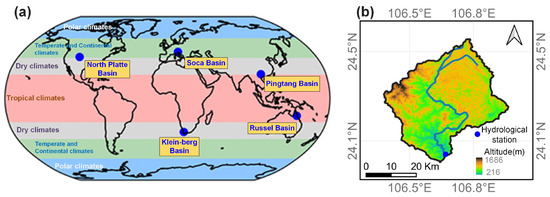
Figure 1.
Approximate profile of the study watersheds: (a) location of the study watersheds in the world map under climate zones and (b) detailed information of the Pingtang watershed. The world map and climate zones were provided by the UK Met Office (www.metoffice.gov.uk; last accessed on 31 August 2023).
To further test the effectiveness of the EC approach, we conducted tests on five watersheds (including the Pingtang Watershed) with different hydrometeorological features (Table 1). These watersheds were selected as they have sufficient runoff data (daily missing = 0 during 2003–2018) for model calibration and validation. The area of these watersheds is approximately distributed between 300 and 60,000 km2. Meanwhile, the climate types of these watersheds cover dry, tropical, temperate, and continental climates. The runoff and geographic boundary data of these study watersheds (except for the Pingtang Watershed) were downloaded from the global runoff data center, and their quality has been controlled by the World Meteorological Organization. The approximate locations and hydrometeorological features of these watersheds are shown in Figure 1a and Table 1, respectively.

Table 1.
Summary of hydrometeorological features for the study watersheds.
2.2. Multiple Remotely Sensed Precipitation Datasets (RSPDs)
The precipitation datasets were selected based on the following criteria: (1) open access, (2) spatial resolution ≤ 0.25°, (3) temporal resolution ≤ 1 day, (4) continuous update, and (5) global coverage (spatial extent ≥ 50° N/S). These criteria are applied to ensure that each product is suitable for use in a variety of terrains, including plains and mountainous areas, as well as to support practical applications, including runoff forecasting and reproduction. Meanwhile, for the same family of products, the gauge enhancement version was adopted because of its reduced systematic bias. Finally, six precipitation datasets were adopted. Specific information about these RSPDs is summarized in Table 2.
Table 2.
Overview of the precipitation datasets adopted in this study. The abbreviation NRT in the temporal range/resolution column stands for near real-time.
CHIRPS is a quasi-global precipitation dataset, and it combines satellite imagery, gauge measurements, and high-resolution precipitation climatology to produce gridded precipitation estimates. CHIRPS V 2.0 is an enhanced version by using increased (~13,900) stations. This dataset is available at daily scales and 0.05° spatial resolutions. IMERG combines information from the GPM satellite constellation, using the Goddard Profiling Algorithm to compute precipitation estimates [19]. Meanwhile, IMERG is available in three versions: Early, Late, and Final Runs, which differ in the latency and input data sources. The IMERG Final Run (V6.0) was collected in this study from the NASA website (Table 2). CMORPH is a satellite precipitation product that uses the morphing technique to estimate global precipitation. In particular, the CMORPH gauge blended version was collected in this study for its reduced systematic bias. GSMaP is a product of the Global Precipitation Measurement mission, which aims to improve the understanding and prediction of the global water cycle and weather. The V6.0 gauge-adjusted GSMaP was adopted in this study. PERSIANN combines information from passive microwave and infrared sensors on multiple satellites, using a cloud classification scheme and a precipitation retrieval model. PERSIANN has different versions and resolutions, such as PERSIANN-CCS and PERSIANN-CDR. Among PERSIANN products, the PERSIANN-CDR is an improved version using radar and hourly rain gauge data. MSWX is a high-resolution (3-hourly 0.1°) meteorological product that provides global coverage of 10 near-surface variables, including precipitation, air temperature, and surface pressure. Compared to ERA5, the MSWX has a better performance and reduced systematic bias [23]. The MSWX-PAST version spans from 1981 to the present, and its reliability has been validated in global and regional applications [23,47]. It is important to note that satellite information has been applied directly (or indirectly) to all of these products. For example, satellite information was used in ERA5 to improve initial conditions. Therefore, for the sake of convenience, all these products are collectively referred to as remotely sensed precipitation datasets.
In summary, these datasets offer continuous precipitation information with high temporal and spatial resolution and global coverage. However, the production strategists used in these datasets vary significantly, especially regarding the precipitation retrieval algorithm (Table 2). These differences may considerably affect the performance of various datasets. Therefore, it is essential to investigate the potential of these precipitation datasets in runoff modeling.
2.3. Potential Evaporation Product
Potential evapotranspiration is also an important input needed for runoff modeling. In this study, we used the potential evapotranspiration data provided by GLEAM (https://www.gleam.eu/; last accessed on 15 May 2023) [48], which covers a long period with a spatial resolution of 0.25°. This product applies the Priestley–Taylor formula to invert the potential evapotranspiration over land. Meanwhile, it is available in two versions (V3.7a and V3.7b), which differ in the temporal coverage and input data sources. GLEAM v3.7a is a global dataset spanning 43 years from 1 January 1980 to 31 December 2022, and GLEAM v3.7b is a dataset spanning 20 years from 1 January 2003 to 31 December 2022. GLEAM v3.7a was adopted in this study for its longer period of coverage.
2.4. Data Pre-Processing and Experimental Period
This study was conducted at a daily spatial resolution and watershed scale for the period of 2003–2018. Therefore, all RSPDs were pre-processed to daily resolution by aggregating sub-daily data. Meanwhile, we applied the average of the precipitation dataset cells within the study watersheds to create watershed-scale precipitation estimates because of the internal resolution consistency of each dataset. Consequently, six basin-scale precipitation time series data that correspond to the adopted precipitation datasets were generated. The runoff and precipitation data from 2003 to 2012 were used for model calibration, while data from 2013 to 2018 was used for model validation.
3. Methodology
The principal methodology used in this study can be divided into three parts: (1) GR4J was used as a representative hydrological model to reproduce runoff, and the GLEAM product and multiple precipitation datasets were used as the inputs of GR4J; (2) the proposed EC approach was used to incorporate the reproduced runoff for enhancing accuracy, and the single precipitation dataset-based approaches and the ensemble average were used as benchmarks; (3) collective approaches, including three metrics, were applied to evaluate the performance of various models.
3.1. The GR4J Model and Its Parameter Determination
GR4J is a daily lumped precipitation-runoff model that originates from Cemagref [49]. It has been validated in more than 400 regions with different hydrological conditions in France, Australia, and other countries. The GR4J model adopts two nonlinear reservoirs for precipitation-runoff modeling, of which the first reservoir represents the production process, and the second reservoir is employed to conceptualize the confluent process. The GR4J contains only four parameters (Table 3). Meanwhile, the model does not rely on geographic observations of the target watershed and is therefore suitable for runoff modeling in remote mountainous and data-poor areas. In this study, the GR4J was calibrated by using the Shuffled Complex Evolution Algorithm with the Nash–Sutcliffe efficiency as a fitness function. Meanwhile, the GR4J calibration for various precipitation datasets was carried out in parallel. The repetitions of the calibration were set as 10,000 times, and the parameter intervals are summarized in Table 3.
Table 3.
Value interval of GR4J parameters for calibration.
3.2. The EC Approach and Its Procedure
To incorporate the reproduced runoff information from the GR4J model and multiple remotely sensed precipitation datasets, this study developed the EC approach. It comprises two components, namely, the ensemble average and the cumulative distribution correction. The core mathematical ideas and physical background are as follows: (i) various precipitation datasets have different biases in a specific precipitation event and, hence, the biases propagation can be mitigated by incorporating the reproduced runoff from different datasets; (ii) there are no significant hydroclimatic disturbances of the target watersheds and, therefore, the model parameters are stationary over the experimental period and the cumulative distribution of runoff is characterized by consistency across temporal periods; (iii) precipitation input is a major source of uncertainty and, thus, there are similar errors between the calibration and validation stages. These ideas have also been partially adopted by previous studies [9,50]. The rationale and limitations of these ideas are elaborated in detail using a case study in Section 4.1 and a discussion in Section 5, respectively. The EC procedure is shown in Figure 2, and the detailed process of the EC is as follows:
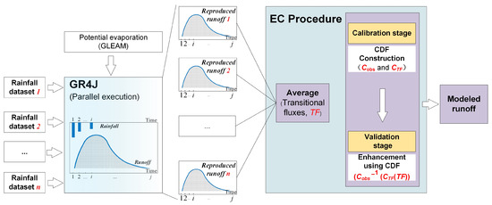
Figure 2.
Procedure overview of the EC approach for incorporating information from the GR4J model and multiple precipitation datasets, where C and CDF are abbreviations for Cumulative Probability Density Function; the subscripts obs and TF represent the observed runoff and transitional fluxes, respectively.
The runoff information reproduced by the n precipitation datasets driving the GR4J model is defined as {}. These reproduced runoffs are averaged to construct transitional fluxes (), which are formulated as follows:
The transitional fluxes and measured runoff during the calibration stage are used to construct empirical and , respectively. CDF are abbreviations for Cumulative Distribution Function.
These empirical cumulative distributions are used to enhance the transitional fluxes during the validation stage, and the process can be formulated as follows:
Finally, the complete form of the EC approach is developed as follows:
where is the modeled runoff in the period ; and represents the empirical cumulative distribution function and its inverse function, respectively; the subscripts and are the modeled and measured runoff, respectively. Overall, the EC method is still simple and easy to use without increasing observed hydrogeographic data.
3.3. Performance Metrics
The Nash–Sutcliffe efficiency (NSE), mean absolute error (MAE), and root mean square error (RMSE) were used as performance metrics. These metrics were adopted based on research practices [50,51]. Among these metrics, the NSE normalizes model performance into an interpretable scale, and NSE = 0 is regularly used as a benchmark to distinguish “good” and “bad” models [52]. MAE is useful when the distribution of the model errors is uniform, while RMSE is largely applicable when the distribution is normal [53]. The definitions of these indicators are as follows:
where and denote the observed and modeled runoff, respectively; N indicates the evaluation sample size. NSE compares the mean square error against observation variance. A higher NSE represents better performance, and the perfect value is 1. The value of NSE is positive (negative) when modeled runoff outperforms (underperforms) reference, taking the form of the mean value of observations. RMSE and MAE are non-negative metrics with an unbiased value of 0.
3.4. Experimental Procedures
This study was conducted following the experimental procedures as shown in Figure 3. Firstly, the reproduced runoff information from GR4J and different precipitation datasets was visualization surveys and preliminary presentations to show its characteristics and errors during calibration and validation stages. Secondly, EC was compared with the single precipitation dataset-based approaches and the ensemble average method using various performance metrics to show the EC’s superiorities under various scenarios. Finally, the superiorities and transferability of EC were verified in watersheds of different hydrometeorological features.
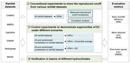
Figure 3.
Schematic workflow of experimental approaches.
4. Results
4.1. The Reproduced Runoff from GR4J and Different Precipitation Datasets
Six precipitation datasets were used separately to drive the GR4J model to reproduce the daily runoff of the Pingtang Watershed. Figure 4 shows these reproduced runoffs for the calibration stage (2003–2012) and validation stage (2013–2018). Generally, all the single precipitation dataset-based approaches tended to have a high uncertainty on high-value runoff events. However, the biases of reproduced runoff based on different precipitation products are anisotropic for localized events in some periods. For instance, around July 2017, the CMORPH- and MSWX-based approaches tended to underestimate and overestimate runoff, respectively. Similarly, around July 2013, there was an overestimation of the PERSIANN-based approach but an underestimation of the CMORPH-based strategy. This anisotropic bias phenomenon suggests that incorporating the reproduced runoff information from various precipitation datasets may be able to improve accuracy. In addition, there are similar biases between the calibration and validation stages. For example, all approaches underestimate runoff around July 2018 in the validation stage and around July 2007 in the calibration period. Overall, although there were errors in these reproduced runoffs, the single precipitation dataset-based approaches reproduced the seasonal fluctuations very well, indicating great value in supporting practical applications.
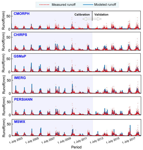
Figure 4.
The modeled runoff driven by different precipitation datasets during the calibration and validation stages for the Pingtang Watershed.
A correlation plot was used to further analyze these single precipitation dataset-based approaches (Figure 5). As can be seen from Figure 5, there was a clear tendency for the single precipitation dataset-based approaches to underestimate runoff. Specifically, at the validation stage, the regression coefficients between reproduced and measured runoffs in the scenarios based on CMORPH, CHIRPS, and GSMaP are 0.21, 0.59, and 0.56, respectively, which were lower than the ideal coefficient 1. These underestimates were also observed in other single precipitation dataset-based approaches (i.e., IMERG, PERSIANN, and MSWX), suggesting that the precipitation input is a major source of uncertainty. In addition, the errors were highly similar for the calibration and validation periods, reaffirming that precipitation inputs are a key source of uncertainty in runoff modeling. Overall, the errors of reproduced runoffs are characterized by consistency across temporal periods. Therefore, it is worthwhile to further explore the value of these reproduced runoffs to enhance accuracy by information incorporation.
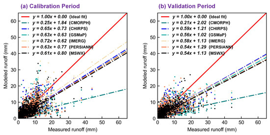
Figure 5.
Scatterplot of the single precipitation dataset-based approaches during the calibration and validation periods for the Pingtang Watershed.
4.2. Superiorities Investigation of the EC Approach
The EC method was used to incorporate reproduced runoff information (Figure 4) from the GR4J hydrological model and six remotely sensed precipitation datasets. Meanwhile, the ensemble average and the single precipitation dataset-based approaches were used as benchmarks. Figure 6 shows an initial indication of the overall accuracy of these approaches. A closer distance between the point representing the approaches and the point representing the runoff observations indicates a higher performance. As can be seen in Figure 6, among the single dataset-based approaches, the IMERG-based approach had the best performance. The EC demonstrated better performance than the ensemble average and all the single precipitation dataset-based approaches for both the calibration and validation stages, suggesting a robust superiority of the EC approach. Overall, the ensemble averaging approach possessed a higher correlation than the single dataset-based approaches, indicating the value of integrating information from multiple sources. However, the spread between the measured values and the standard deviation based on the ensemble average is pronounced and even worse than the single dataset-based approaches. Therefore, it is necessary to further compare the performance of different models using performance metrics.
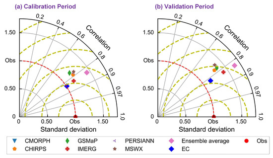
Figure 6.
Taylor chart of eight approaches during calibration and validation periods for the Pingtang Watershed.
Table 4 summarizes the statistical performance metrics of different models for calibration and validation stages. Generally, all approaches exhibited outstanding performance (NSE ≥ 0.34). Among the single dataset-based approaches, the IMERG-based approach exhibited the best performance during both the calibration and validation stages. Meanwhile, the CMORPH-based approach showed the worst performance, with the smallest NSE values as well as the largest MAE and RMSE values. The ensemble averaging approach tended to have better overall performance than most of the single precipitation dataset-based approaches, including CMORPH, CHIRPS, GSMaP, and PERSIANN. However, the ensemble averaging had a worse performance than the IMERG-based approach. This phenomenon suggests the unstable superiority of ensemble averaging with respect to the single precipitation dataset-based approaches. As a comparison, the EC approach demonstrated robust superiority compared to all other approaches. Specifically, at the validation stage, the EC approach had superior performance metric values, acquiring good NSE, MAE, and RMSE values of 0.68, 1.32, and 2.45, respectively, which improves the NSE, MAE, and RMSE by 6.25%, 7%, and 4.67%, respectively, compared with the ensemble average. Therefore, the EC approach is an effective option to enhance runoff modeling.
Table 4.
Statistical metrics for various approaches during calibration and validation stages for Pingtang Watersheds.
The effectiveness of incorporation approaches (i.e., EC and ensemble average) is directly related to their incorporation membership. Therefore, the performance differences between the EC method and the ensemble average were further investigated under various incorporation scenarios. We randomly resampled the six incorporation memberships (Figure 4) to form four incorporation scenarios, with two to five memberships in each scenario (Figure 7). Scenarios P2, P2, P3, P4, and P5 represent incorporation memberships of 2, 3, 4, and 5, respectively. As shown in Figure 7, the number of incorporated memberships has a significant effect on runoff modeling accuracy, with scenarios with more members tending to have higher accuracy. For instance, when the membership number is 5 (Scenario P5), the NSE values of the ensemble average are both 0.69 and 0.66 for the calibration and validation stages, respectively. However, when the membership number is 2 (Scenario P2), the NSE values of the ensemble average are 0.57 and 0.54 for the calibration and validation stages, respectively. Overall, the EC exhibited less performance variation across incorporation scenarios than the ensemble average, indicating it has a more stable performance. Meanwhile, at the validation stage, the EC approach had a robust superiority. For example, the NSE values of the EC are 0.63, 0.66, 0.64, and 0.67 for the P2–5 scenarios, respectively, which increases the NSE values by 16.67%, 1.53%, 4.92%, and 1.52% in P2–5 scenarios, respectively, compared with the ensemble average. The above results reaffirm that the EC method had a superior performance to ensemble averaging.
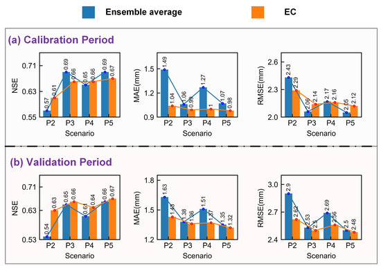
Figure 7.
Comparison of the performance of ensemble average and EC methods under different incorporation scenarios for (a) calibration period and (b) validation period.
4.3. Transferability Verification in Watersheds of Different Hydrometeorological Features
To further test the effectiveness of the EC approach, we conducted tests in five watersheds of different hydrometeorological features (including the Pingtang catchment). The climate types of these watersheds cover four climates. Meanwhile, the area of these watersheds is approximately distributed between 300 and 60,000 km2 (Table 2). Figure 8 shows a radar chart about the accuracy metrics of the eight approaches in the five test watersheds. All approaches exhibited variation in performance from different watersheds, indicating that hydrometeorological characteristics have an important impact on the accuracy of runoff modeling. Overall, the single precipitation dataset-based approaches tended to have higher fluctuations in performance than the incorporation approaches (i.e., ensemble average and EC). For example, the NSE of the GSMaP-based approach ranged from −1.35 to 0.80 and from −0.04 to 0.59 at the calibration and validation stages, respectively. However, the NSE of the ensemble average ranged from 0.31 to 0.75 and from 0.34 to 0.64 at the calibration and validation stages, respectively. Although the MSWX-based approach demonstrated a slight advantage over the incorporation approaches in the So and Kl watersheds, it performed poorly in the NPR watershed and worse than the EC approach in all other watersheds. Therefore, the incorporation approaches exhibited better transferability than single precipitation dataset-based approaches. In addition, at the validation stage, the average NSE of the single precipitation dataset-based approaches is 0.36, which is lower than that of the ensemble average (0.51) and EC (0.63). Furthermore, the NSE values of the EC approach are 0.68, 0.52, 0.64, 0.59, and 0.74 for the Pi, NP, Ru, So, and Kl watersheds, respectively, which increases the NSE values by 5.40%, 53.38%, 36.17%, 4.65%, and 73.84% in the Pi-to-Kl watersheds, respectively, compared with the ensemble average. Therefore, the proposed EC approach achieved reasonable superiority and transferability.
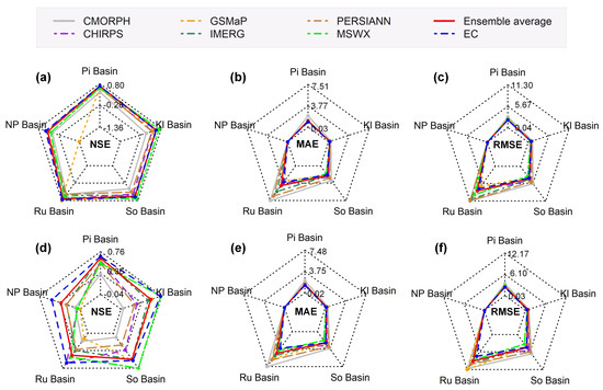
Figure 8.
Radar plots of the performance of the eight runoff modeling strategies in the five test watersheds during the calibration stage: (a) NSE; (b) MAE; (c) RMSE and the validation stage; (d) NSE; (e) MAE; (f) RMSE. The units of the MAE and RMSE metrics are mm.
5. Discussion
A unique aspect of this study is the investigation of six RSPDs in runoff modeling. Therefore, we further discussed the error characteristics and value of RSPDs. The study found that the single precipitation dataset-based approaches tended to underestimate runoff, which is consistent with references [54,55]. This phenomenon may be attributed to error propagation. Specifically, RSPDs suffer from an underestimation of heavy precipitation [56], and this error propagates through the precipitation-runoff process. An indirect evidence to support the above attribution is the significant similarity between the errors in the reproduced runoff during the calibration and calibration stages (Figure 4 and Figure 5). Interestingly, this study found that the single precipitation dataset-based approaches exhibited outstanding performance in reproducing seasonal fluctuations, indicating their great value in supporting long-term applications. In addition, we found that the single precipitation dataset-based approaches have limited transferability (Figure 8). The possible reason is that there are huge regional performance differences in RSPDs [26,57]. For example, IMERG has satisfactory performance in plains but is highly uncertain in mountainous regions [57]. PERSIANN tends to be better and worse than GSMaP in China and CONUS, respectively [57,58]. The incorporation approaches (i.e., ensemble averaging and EC) exhibited better overall performance and transferability than the single precipitation dataset-based approaches (Table 4 and Figure 8). Therefore, the results of this study highlight the value of the incorporation of multiple precipitation datasets in runoff modeling.
The key novelty of this study lies in the development of a two-step approach (i.e., EC) to incorporate information from the GR4J hydrological model and multiple remotely sensed precipitation datasets. Compared to ensemble averaging, the EC method exhibited superior transferability and performance (Figure 8). The possible reason is that a distribution correction process is introduced in the EC method (Equation (2)). Specifically, all the single precipitation dataset-based approaches suffer from a similar underestimation, which would make the performance of ensemble averaging methods unstable (Figure 5 and Table 4). The distribution correction is effective in reducing systematic errors, which in turn may make the EC method perform better than the ensemble average. In addition to runoff modeling, the EC method can also be extended to near real-time runoff forecasts with short lag times consistent with precipitation datasets. Meanwhile, the EC method only relies on reproduced runoff information without increasing observed hydrogeographic data. Therefore, this methodology is valuable and replicable for other regions that are characterized by different hydrometeorological features.
Although this study provides some new insights into the hydrological application of RSPDs and the proposed EC approach has achieved reasonable performance and transferability, some limitations still need to be discussed. The assumptions within EC cover the consistency of hydrometeorological behavior across calibration and validation stages. This assumption has also been adopted in a large number of precipitation-runoff modeling studies [12,50]. However, with global industrialization and geographic resource exploitation, non-stationarity in hydrometeorological behavior has been progressively observed [59]. Severe environmental disturbances can disrupt the statistical distribution of hydrometeorological elements and the consistency of the precipitation-runoff process, which in turn may make the EC no longer applicable. Therefore, it is not realistic to extrapolate the findings of this study to other regions with severe hydrometeorological disturbances. In addition, only global precipitation datasets were considered in the study owing to the need to support transferability testing. However, regional precipitation datasets, e.g., the China Meteorological Forcing Dataset [60], tended to be more accurate in their coverage areas than global precipitation products. Therefore, if the conditions permit, more precipitation datasets can be included to further enhance runoff modeling for a special application.
6. Conclusions
The potential of six remotely sensed precipitation datasets was investigated in runoff modeling, and a new two-step approach (i.e., EC) was proposed to incorporate the reproduced runoff information from these datasets to enhance accuracy. Meanwhile, the single precipitation dataset-based approaches and the ensemble average were used as benchmarks. We found that
- (1)
- The single precipitation dataset-based approaches reproduced the seasonal fluctuations well but tended to have a high uncertainty on high-value runoff events. Meanwhile, these approaches tended to underestimate runoff, and there were similar errors between the calibration and validation stages.
- (2)
- The EC method had a satisfactory performance with Nash–Sutcliffe values of 0.68 during calibration and validation. Meanwhile, the EC method performed better than all the benchmarks and exhibited a more stable performance than the ensemble averaging method under different incorporation scenarios.
- (3)
- Both the EC model and ensemble averaging have good transferability but the EC model has better performance across all test watersheds. However, the single precipitation dataset-based approaches exhibited significant regional variations and, therefore, had low transferability.
The current study highlights the value of the incorporation of multiple precipitation datasets in runoff modeling and provides an effective alternative to enhance accuracy. Further research can be directed to the inclusion of regional precipitation datasets for a special application.
Author Contributions
Data curation, X.L.; Funding acquisition, C.M., R.M., Y.H. and G.S.; Investigation, Q.S. and Y.H.; Methodology, X.L.; Project administration, C.M.; Resources, C.M., R.M., Y.H. and G.S.; Validation, X.L.; Visualization, Q.S. and X.L.; Writing—original draft, X.L.; Writing—review and editing, X.L. and C.F. All authors have read and agreed to the published version of the manuscript.
Funding
This research was funded by the National Natural Science Foundation of China (Grant Nos. 52269002 and 51969004) and the Guangxi Water Resource Technology Promotion Foundation (Grant Nos. SK2022-021 and SK2021-3-23).
Data Availability Statement
The data presented in this study are available on request from the corresponding author. The data are not publicly available due to policy constraints.
Conflicts of Interest
Author Yi Huang was employed by the company Guangxi Water & Power Design Institute Co., Ltd. The remaining authors declare that the research was conducted in the absence of any commercial or financial relationships that could be construed as a potential conflict of interest.
References
- Liu, Y.; Ji, C.; Wang, Y.; Zhang, Y.; Hou, X.; Ma, H. Consideration of streamflow forecast uncertainty in the development of short-term hydropower station optimal operation schemes: A novel approach based on mean-variance theory. J. Clean Prod. 2021, 304, 126929. [Google Scholar] [CrossRef]
- Letcher, R.A.; Croke, B.F.W.; Jakeman, A.J. Integrated assessment modelling for water resource allocation and management: A generalised conceptual framework. Environ. Modell. Softw. 2007, 22, 733–742. [Google Scholar] [CrossRef]
- Stergiadi, M.; Di Marco, N.; Avesani, D.; Righetti, M.; Borga, M. Impact of Geology on Seasonal Hydrological Predictability in Alpine Regions by a Sensitivity Analysis Framework. Water 2020, 12, 2255. [Google Scholar] [CrossRef]
- Niu, W.; Feng, Z. Evaluating the performances of several artificial intelligence methods in forecasting daily streamflow time series for sustainable water resources management. Sust. Cities Soc. 2021, 64, 102562. [Google Scholar] [CrossRef]
- Kuichling, E. The relation between the rainfall and the discharge of sewers in populous districts. Trans. Am. Soc. Civil Eng. 1889, 20, 1–56. [Google Scholar] [CrossRef]
- Peel, M.C.; Mcmahon, T.A. Historical development of rainfall-runoff modeling. Wiley Interdiscip. Rev. Water 2020, 7, e1471. [Google Scholar] [CrossRef]
- Zuo, G.; Luo, J.; Wang, N.; Lian, Y.; He, X. Two-stage variational mode decomposition and support vector regression for streamflow forecasting. Hydrol. Earth Syst. Sci. 2020, 24, 5491–5518. [Google Scholar] [CrossRef]
- Perrin, C.; Michel, C.; Andréassian, V. Improvement of a parsimonious model for streamflow simulation. J. Hydrol. 2003, 279, 275–289. [Google Scholar] [CrossRef]
- Yu, Z.; Wu, J.; Yao, H.; Chen, X.; Cai, Y. Calibrating a hydrological model in ungauged small river basins of the northeastern Tibetan Plateau based on near-infrared images. J. Hydrol. 2023, 618, 129158. [Google Scholar] [CrossRef]
- Ghimire, U.; Agarwal, A.; Shrestha, N.K.; Daggupati, P.; Srinivasan, G.; Than, H.H. Applicability of Lumped Hydrological Models in a Data-Constrained River Basin of Asia. J. Hydrol. Eng. 2020, 25, 05020018. [Google Scholar] [CrossRef]
- Sezen, C.; Bezak, N.; Bai, Y.; Šraj, M. Hydrological modelling of karst catchment using lumped conceptual and data mining models. J. Hydrol. 2019, 576, 98–110. [Google Scholar] [CrossRef]
- Moosavi, V.; Gheisoori Fard, Z.; Vafakhah, M. Which one is more important in daily runoff forecasting using data driven models: Input data, model type, preprocessing or data length? J. Hydrol. 2022, 606, 127429. [Google Scholar] [CrossRef]
- Kidd, C.; Becker, A.; Huffman, G.J.; Muller, C.L.; Joe, P.; Skofronick-Jackson, G.; Kirschbaum, D.B. So, How Much of the Earth’s Surface Is Covered by Rain Gauges? Bull. Amer. Meteorol. Soc. 2017, 98, 69–78. [Google Scholar] [CrossRef]
- Lewis, E.; Fowler, H.; Alexander, L.; Dunn, R.; Mcclean, F.; Barbero, R.; Guerreiro, S.; Li, X.; Blenkinsop, S. GSDR: A Global Sub-Daily Rainfall Dataset. J. Clim. 2019, 32, 4715–4729. [Google Scholar] [CrossRef]
- Sujud, L.H.; Jaafar, H.H. A global dynamic runoff application and dataset based on the assimilation of GPM, SMAP, and GCN250 curve number datasets. Sci. Data 2022, 9, 706. [Google Scholar] [CrossRef] [PubMed]
- Beck, H.E.; Wood, E.F.; Pan, M.; Fisher, C.K.; Miralles, D.G.; van Dijk, A.I.J.M.; Mcvicar, T.R.; Adler, R.F. MSWEP V2 Global 3-Hourly 0.1° Precipitation: Methodology and Quantitative Assessment. Bull. Amer. Meteorol. Soc. 2019, 100, 473–500. [Google Scholar] [CrossRef]
- Sun, Q.; Miao, C.; Duan, Q.; Ashouri, H.; Sorooshian, S.; Hsu, K.L. A Review of Global Precipitation Data Sets: Data Sources, Estimation, and Intercomparisons. Rev. Geophys. 2018, 56, 79–107. [Google Scholar] [CrossRef]
- Funk, C.; Peterson, P.; Landsfeld, M.; Pedreros, D.; Verdin, J.; Shukla, S.; Husak, G.; Rowland, J.; Harrison, L.; Hoell, A.; et al. The climate hazards infrared precipitation with stations-a new environmental record for monitoring extremes. Sci. Data 2015, 2, 150066. [Google Scholar] [CrossRef] [PubMed]
- Huffman, G.J.; Bolvin, D.T.; Braithwaite, D.; Hsu, K.; Joyce, R.J.; Kidd, C.; Nelkin, E.J.; Sorooshian, S.; Stocker, E.F.; Tan, J.; et al. Integrated Multi-satellite Retrievals for the Global Precipitation Measurement (GPM) Mission (IMERG). In Satellite Precipitation Measurement: Volume 1; Levizzani, V., Kidd, C., Kirschbaum, D.B., Kummerow, C.D., Nakamura, K., Turk, F.J., Eds.; Springer International Publishing: Cham, Switzerland, 2020; pp. 343–353. ISBN 978-3-030-24568-9. [Google Scholar]
- Joyce, R.J.; Janowiak, J.E.; Arkin, P.A.; Xie, P. CMORPH: A Method that Produces Global Precipitation Estimates from Passive Microwave and Infrared Data at High Spatial and Temporal Resolution. J. Hydrometeorol. 2004, 5, 487–503. [Google Scholar] [CrossRef]
- Mega, T.; Ushio, T.; Takahiro, M.; Kubota, T.; Kachi, M.; Oki, R. Gauge-Adjusted Global Satellite Mapping of Precipitation. IEEE Trans. Geosci. Remote Sens. 2019, 57, 1928–1935. [Google Scholar] [CrossRef]
- Ashouri, H.; Hsu, K.; Sorooshian, S.; Braithwaite, D.K.; Knapp, K.R.; Cecil, L.D.; Nelson, B.R.; Prat, O.P. PERSIANN-CDR: Daily Precipitation Climate Data Record from Multisatellite Observations for Hydrological and Climate Studies. Bull. Amer. Meteorol. Soc. 2015, 96, 69–83. [Google Scholar] [CrossRef]
- Beck, H.E.; van Dijk, A.I.J.M.; Larraondo, P.R.; Mcvicar, T.R.; Pan, M.; Dutra, E.; Miralles, D.G. MSWX Global 3-Hourly 0.1° Bias-Corrected Meteorological Data Including Near-Real-Time Updates and Forecast Ensembles. Bull. Amer. Meteorol. Soc. 2022, 103, 710–732. [Google Scholar] [CrossRef]
- Liao, M.; Barros, A.P. Toward optimal rainfall—Hydrologic QPE correction in headwater basins. Remote Sens. Environ. 2022, 279, 113107. [Google Scholar] [CrossRef]
- Wu, W.; Yang, Z.; Zhao, L.; Lin, P. The impact of multi-sensor land data assimilation on river discharge estimation. Remote Sens. Environ. 2022, 279, 113138. [Google Scholar] [CrossRef]
- Beck, H.E.; Vergopolan, N.; Pan, M.; Levizzani, V.; van Dijk, A.I.J.M.; Weedon, G.P.; Brocca, L.; Pappenberger, F.; Huffman, G.J.; Wood, E.F. Global-scale evaluation of 22 precipitation datasets using gauge observations and hydrological modeling. Hydrol. Earth Syst. Sci. 2017, 21, 6201–6217. [Google Scholar] [CrossRef]
- Mei, Y.; Nikolopoulos, E.I.; Anagnostou, E.N.; Borga, M. Evaluating Satellite Precipitation Error Propagation in Runoff Simulations of Mountainous Basins. J. Hydrometeorol. 2016, 17, 1407–1423. [Google Scholar] [CrossRef]
- Tang, G.; Clark, M.P.; Knoben, W.J.M.; Liu, H.; Gharari, S.; Arnal, L.; Beck, H.E.; Wood, A.W.; Newman, A.J.; Papalexiou, S.M. The Impact of Meteorological Forcing Uncertainty on Hydrological Modeling: A Global Analysis of Cryosphere Basins. Water Resour. Res. 2023, 59, e2022WR033767. [Google Scholar] [CrossRef]
- Ehsan Bhuiyan, M.A.; Nikolopoulos, E.I.; Anagnostou, E.N.; Polcher, J.; Albergel, C.; Dutra, E.; Fink, G.; Martínez-De La Torre, A.; Munier, S. Assessment of precipitation error propagation in multi-model global water resource reanalysis. Hydrol. Earth Syst. Sci. 2019, 23, 1973–1994. [Google Scholar] [CrossRef]
- Liu, J.; Yuan, X.; Zeng, J.; Jiao, Y.; Li, Y.; Zhong, L.; Yao, L. Ensemble streamflow forecasting over a cascade reservoir catchment with integrated hydrometeorological modeling and machine learning. Hydrol. Earth Syst. Sci. 2022, 26, 265–278. [Google Scholar] [CrossRef]
- Zhu, S.; Wei, J.; Zhang, H.; Xu, Y.; Qin, H. Spatiotemporal deep learning rainfall-runoff forecasting combined with remote sensing precipitation products in large scale basins. J. Hydrol. 2023, 616, 128727. [Google Scholar] [CrossRef]
- Jiang, S.; Ren, L.; Hong, Y.; Yong, B.; Yang, X.; Yuan, F.; Ma, M. Comprehensive evaluation of multi-satellite precipitation products with a dense rain gauge network and optimally merging their simulated hydrological flows using the Bayesian model averaging method. J. Hydrol. 2012, 452, 213–225. [Google Scholar] [CrossRef]
- Koster, T.; El-Serafy, G.; van den Boogaard, H.; Heemink, A.W.; Mynett, A. Input correction in rainfall runoff models using the Ensemble Kalman filter. In Proceedings of the 4th International Symposium on Environmental Hydraulics, Hong Kong, China, 15–18 December 2004. [Google Scholar]
- Hazra, A.; Maggioni, V.; Houser, P.; Antil, H.; Noonan, M. A Monte Carlo-based multi-objective optimization approach to merge different precipitation estimates for land surface modeling. J. Hydrol. 2019, 570, 454–462. [Google Scholar] [CrossRef]
- Lei, H.; Zhao, H.; Ao, T. A two-step merging strategy for incorporating multi-source precipitation products and gauge observations using machine learning classification and regression over China. Hydrol. Earth Syst. Sci. 2022, 26, 2969–2995. [Google Scholar] [CrossRef]
- Sharma, N.; Zakaullah, M.; Tiwari, H.; Kumar, D. Runoff and sediment yield modeling using ANN and support vector machines: A case study from Nepal watershed. Model. Earth Syst. Environ. 2015, 1, 23. [Google Scholar] [CrossRef]
- Jia, Y.; Song, S.; Ge, L. Trimmed L-Moments of the Pearson Type III Distribution for Flood Frequency Analysis. Water Resour. Manag. 2023, 37, 1321–1340. [Google Scholar] [CrossRef]
- Qi, L.; Yu, H.; Chen, P. Selective ensemble-mean technique for tropical cyclone track forecast by using ensemble prediction systems. Q. J. R. Meteorol. Soc. 2014, 140, 805–813. [Google Scholar] [CrossRef]
- Van Loon, A.F.; Van Huijgevoort, M.H.J.; Van Lanen, H.A.J. Evaluation of drought propagation in an ensemble mean of large-scale hydrological models. Hydrol. Earth Syst. Sci. 2012, 16, 4057–4078. [Google Scholar] [CrossRef]
- Kasiviswanathan, K.S.; Cibin, R.; Sudheer, K.P.; Chaubey, I. Constructing prediction interval for artificial neural network rainfall runoff models based on ensemble simulations. J. Hydrol. 2013, 499, 275–288. [Google Scholar] [CrossRef]
- Mo, C.; Liu, G.; Lei, X.; Zhang, M.; Ruan, Y.; Lai, S.; Xing, Z. Study on the Optimization and Stability of Machine Learning Runoff Prediction Models in the Karst Area. Appl. Sci. 2022, 12, 4979. [Google Scholar] [CrossRef]
- Strauch, M.; Bernhofer, C.; Koide, S.; Volk, M.; Lorz, C.; Makeschin, F. Using precipitation data ensemble for uncertainty analysis in SWAT streamflow simulation. J. Hydrol. 2012, 414, 413–424. [Google Scholar] [CrossRef]
- Mo, C.; Cen, W.; Lei, X.; Ban, H.; Ruan, Y.; Lai, S.; Shen, Y.; Xing, Z. Simulation of dam-break flood and risk assessment: A case study of Chengbi River Dam in Baise, China. J. Hydroinform. 2023, 25, 1276–1294. [Google Scholar] [CrossRef]
- Zhang, X. Evaluation of design flood estimates in karst areas–a case study of Chengbi river. J. China Hydrol. 1994, 2, 30–33. [Google Scholar] [CrossRef]
- Jiang, H.; Yu, Z.; Mo, C. Ensemble Method for Reservoir Flood Season Segmentation. J. Water Resour. Plan. Manag.-Asce 2017, 143, 04016079. [Google Scholar] [CrossRef]
- Mo, C.; Lai, S.; Yang, Q.; Huang, K.; Lei, X.; Yang, L.; Yan, Z.; Jiang, C. A comprehensive assessment of runoff dynamics in response to climate change and human activities in a typical karst watershed, southwest China. J. Environ. Manag. 2023, 332, 117380. [Google Scholar] [CrossRef]
- Araghi, A.; Martinez, C.J.; Olesen, J.E. Evaluation of MSWX gridded data for modeling of wheat performance across Iran. Eur. J. Agron. 2023, 144, 126769. [Google Scholar] [CrossRef]
- Martens, B.; Miralles, D.G.; Lievens, H.; van der Schalie, R.; de Jeu, R.A.M.; Fernández-Prieto, D.; Beck, H.E.; Dorigo, W.A.; Verhoest, N.E.C. GLEAM v3: Satellite-based land evaporation and root-zone soil moisture. Geosci. Model Dev. 2017, 10, 1903–1925. [Google Scholar] [CrossRef]
- Edijatno; DE Oliveira Nascimento, N.; Yang, X.; Makhlouf, Z.; Michel, C. GR3J: A daily watershed model with three free parameters. Hydrol. Sci. J. 1999, 44, 263–277. [Google Scholar] [CrossRef]
- Dou, Y.; Ye, L.; Gupta, H.V.; Zhang, H.; Behrangi, A.; Zhou, H. Improved Flood Forecasting in Basins With No Precipitation Stations: Constrained Runoff Correction Using Multiple Satellite Precipitation Products. Water Resour. Res. 2021, 57, e2021WR029682. [Google Scholar] [CrossRef]
- Huang, Z.; Zhao, T. Predictive performance of ensemble hydroclimatic forecasts: Verification metrics, diagnostic plots and forecast attributes. Wiley Interdiscip. Rev. Water 2022, 9, e1580. [Google Scholar] [CrossRef]
- Knoben, W.J.M.; Freer, J.E.; Woods, R.A. Technical note: Inherent benchmark or not? Comparing Nash-Sutcliffe and Kling-Gupta efficiency scores. Hydrol. Earth Syst. Sci. 2019, 23, 4323–4331. [Google Scholar] [CrossRef]
- Chai, T.; Draxler, R.R. Root mean square error (RMSE) or mean absolute error (MAE)?—Arguments against avoiding RMSE in the literature. Geosci. Model Dev. 2014, 7, 1247–1250. [Google Scholar] [CrossRef]
- Getirana, A.; Kirschbaum, D.; Mandarino, F.; Ottoni, M.; Khan, S.; Arsenault, K. Potential of GPM IMERG Precipitation Estimates to Monitor Natural Disaster Triggers in Urban Areas: The Case of Rio de Janeiro, Brazil. Remote Sens. 2020, 12, 4095. [Google Scholar] [CrossRef]
- Yuan, F.; Wang, B.; Shi, C.; Cui, W.; Zhao, C.; Liu, Y.; Ren, L.; Zhang, L.; Zhu, Y.; Chen, T.; et al. Evaluation of hydrological utility of IMERG Final run V05 and TMPA 3B42V7 satellite precipitation products in the Yellow River source region, China. J. Hydrol. 2018, 567, 696–711. [Google Scholar] [CrossRef]
- Chen, H.; Wen, D.; Du, Y.; Xiong, L.; Wang, L. Errors of five satellite precipitation products for different rainfall intensities. Atmos. Res. 2023, 285, 106622. [Google Scholar] [CrossRef]
- Beck, H.E.; Pan, M.; Roy, T.; Weedon, G.P.; Pappenberger, F.; van Dijk, A.I.J.M.; Huffman, G.J.; Adler, R.F.; Wood, E.F. Daily evaluation of 26 precipitation datasets using Stage-IV gauge-radar data for the CONUS. Hydrol. Earth Syst. Sci. 2019, 23, 207–224. [Google Scholar] [CrossRef]
- Wang, Y.; Zhao, N. Evaluation of Eight High-Resolution Gridded Precipitation Products in the Heihe River Basin, Northwest China. Remote Sens. 2022, 14, 1458. [Google Scholar] [CrossRef]
- Yang, Y.; Roderick, M.L.; Yang, D.; Wang, Z.; Ruan, F.; Mcvicar, T.R.; Zhang, S.; Beck, H.E. Streamflow stationarity in a changing world. Environ. Res. Lett. 2021, 16, 64096. [Google Scholar] [CrossRef]
- He, J.; Yang, K.; Tang, W.; Lu, H.; Qin, J.; Chen, Y.; Li, X. The first high-resolution meteorological forcing dataset for land process studies over China. Sci. Data 2020, 7, 25. [Google Scholar] [CrossRef]
Disclaimer/Publisher’s Note: The statements, opinions and data contained in all publications are solely those of the individual author(s) and contributor(s) and not of MDPI and/or the editor(s). MDPI and/or the editor(s) disclaim responsibility for any injury to people or property resulting from any ideas, methods, instructions or products referred to in the content. |
© 2024 by the authors. Licensee MDPI, Basel, Switzerland. This article is an open access article distributed under the terms and conditions of the Creative Commons Attribution (CC BY) license (https://creativecommons.org/licenses/by/4.0/).