Article

Phreatic Line Calculation of Reservoir Landslide under Complex Hydraulic Conditions—A Case Study

1
Technology Innovation Center for Geohazard Monitoring and Risk Early Warning, Beijing 100084, China
2
Key Laboratory of Ministry of Education for Geomechanics and Embankment Engineering, Hohai University, Nanjing 210023, China
3
School of Water Resources and Environment, China University of Geosciences, Beijing 100084, China
4
School of Civil Engineering, Suzhou University of Science and Technology, Suzhou 215011, China
5
School of Resources and Environmental Engineering, Hefei University of Technology, Hefei 230009, China
*
Author to whom correspondence should be addressed.
Water 2024, 16(3), 375; https://doi.org/10.3390/w16030375
Submission received: 15 December 2023 / Revised: 11 January 2024 / Accepted: 21 January 2024 / Published: 23 January 2024
(This article belongs to the Special Issue Recent Research on Reservoir Landslide Stability)

Abstract

:
A seepage field, influenced by rainfall and reservoir water level fluctuation, is closely associated with the stability of the reservoir landslide. Understanding the phreatic line variation inside the landslide is of significant importance for the analysis and evaluation of slope stability. Currently, most of the boundaries of phreatic line analytical models and the hydrological conditions are simplified, resulting in discrepancies between the outcomes derived from these models and the actual situation. Given this, the newly proposed analytical model is refined by addressing the following two issues. Firstly, the consideration of variable-speed reservoir level fluctuations is incorporated, and secondly, the reservoir bank within the water-level fluctuation zone is treated as non-vertical. Under the combined effect of reservoir water level fluctuation and rainfall, the Boussinesq Differential Equation of unsteady seepage is established and applied to the Majiagou landslide in Three Gorges reservoir area. The results of the analytical solution are basically consistent with the measured groundwater level results, which has demonstrated the accuracy of the proposed model. Consequently, the proposed model can quickly and accurately calculate the groundwater level of landslides, which provides an effective means for the prediction and early warning of reservoir landslides.

1. Introduction

Since the completion of the Three Gorges Dam in 2003, a total of 4429 geologic hazards have been identified in the Three Gorges Region (TGR) [1]. Compared with other types of landslides, the failure of a reservoir landslide will not only pose a direct threat to the lives and property of the residents, but also induce secondary surge waves, which can cause serious harm to the downstream roads, bridges, housing and other facilities [2,3,4,5,6]. In October 1963, the failure of the Italy Vaiont landslide was triggered, and about 2 billion cubic meters of the mountain mass ran into the reservoir. This event induced nearly 250 m high surge waves, resulting in the direct destruction of downstream villages and towns and causing a tragic loss of approximately 2000 lives [7,8,9,10]. In July 2003, with the reservoir’s water level reaching 135 m, the failure of Qianjiangping landslide occurred. The volume of the Qianjiangping landslide was approximately 15 million cubic meters, precipitating a surge of 24.5 m. This event led to 14 deaths [11,12].
The evolution of the seepage field within reservoir landslides is intricately influenced by rainfall and reservoir water level fluctuation [13,14,15,16,17]. This dynamic interplay disrupts the pre-existing equilibrium of the landslide, thereby exerting a consequential impact on its stability [18,19,20,21,22,23,24,25,26]. Particularly, the phreatic line serves as an effective delineator of seepage flow information within the landslide. Consequently, how to accurately calculate the phreatic line of landslides has become a hot topic. Physical model tests, numerical simulation and analytical methods are the most commonly used methods to solve landslide phreatic lines [27,28,29]. Many scholars have carried out studies through physical model tests and numerical simulation, and a series of achievements have been made [30,31,32,33,34]. However, numerical methods often entail substantial computational time, and physical model tests consume a lot of manpower and material resources. Alternatively, employing an analytical solution method necessitates the adoption of certain assumptions so as to derive an exact solution. In cases where these assumptions hold valid, the analytical solution proves to be a straightforward and pragmatic approach for exploring the phreatic line variation within the reservoir landslide.
Based on the Boussinesq’s Differential Equation of unsteady seepage, a simplified formula of the phreatic line calculation in landslide stability evaluation was proposed during reservoir drawdown [35]. Wu et al. (2007, 2009) elucidated an approximate analytical solution for the phreatic line within the context of a homogeneous bank slope model featuring a water-resistant foundation characterized by a gentle dip angle [36,37]. This solution comprehensively incorporated the combined effect of reservoir water level fluctuation and rainfall. Subsequently, an analysis of the analytical solution of the phreatic line was carried out under the combined effect of rainfall and a constant velocity change of the reservoir water level [38,39,40]. Despite the extensive efforts invested by numerous scholars in the analytical investigation of the landslide phreatic line under the joint influence of rainfall and reservoir water level fluctuation, the prevailing models still have the following limitations. Primarily, certain researchers have simplified the boundary conditions by presuming that the initial water table is horizontally oriented and the bank slope within the water-level fluctuation zone is vertical, a simplification that deviates significantly from the actual scenario. Furthermore, the assumption that the fluctuation rate of the reservoir water level is constant does not align with the dynamic nature of reservoir water level fluctuation, wherein the fluctuation rate is changing with time.
In this study, based on the Boussinesq Differential Equation of unsteady seepage theory, a new phreatic line analytical model was proposed, considering the initial boundary condition and actual reservoir water level fluctuation. Subsequently, the proposed model was applied to a traditional reservoir landslide—the Majiagou landslide. The derived analytical results were compared against the measured results, and the feasibility and accuracy of the proposed method were demonstrated.

2. Method

Given that the governing equation of the Boussinesq method is a second-order non-homogeneous partial differential equation, the attainment of an analytical solution for the phreatic line necessitates the imposition of certain assumptions and linearization of the equation [35]. In the course of solving the groundwater phreatic line, the Dupuit Assumption is incorporated, stipulating that the water head in the landslide is constant in the vertical direction, with the seepage flow rate being significantly smaller than the horizontal flow rate. The fundamental assumptions delineated in this study are listed as follows.

2.1. Basic Assumptions

(1) The aquifer is assumed to be isotropic and homogeneous, possessing infinite lateral extension, and featuring a horizontal impermeable layer;
(2) The flow within the aquifer is assumed to be one-dimensional;
(3) The bank slope within the water-level fluctuation zone is considered with respect to its actual geometric inclination;
(4) Prior to the change in reservoir water level, groundwater flow within the reservoir bank slope is assumed to be steady;
(5) The fluctuation rate of the reservoir water level is in accordance with actual conditions;
(6) Groundwater flow within soil is considered as saturated seepage.
In instances characterized by unsteady seepage flow, the analytical derivation of the phreatic line, under the combined influence of reservoir water level fluctuation and rainfall, the foundational differential equation governing the one-dimensional unsteady motion of Boussinesq phreatic water can be established as follows:
μ H t = x ( K h H x ) + W ,
where H denotes water head (m); h denotes aquifer thickness (m); K denotes the aquifer permeability coefficient (m/d); x denotes the horizontal distance of the calculated point to the origin (m); μ denotes the gravity water yield; W denotes rainfall intensity (m/d); t denotes the duration of time (d).

2.2. Simplification of Differential Equations
In the actual situation, although there will be some changes in the thickness of aquifer h, these changes are relatively small in the space-time scale and can be almost ignored. Consequently, for analytical purposes, the aquifer thickness h is treated as a constant parameter, replaced by the average thickness hm of the phreatic flow at the beginning and end time of the time interval:
H t = K h m μ 2 H x 2 + W μ ,
Defining α = K h m μ , β = W μ , Equation (2) can be modified as:
H t = α 2 H x 2 + β ,
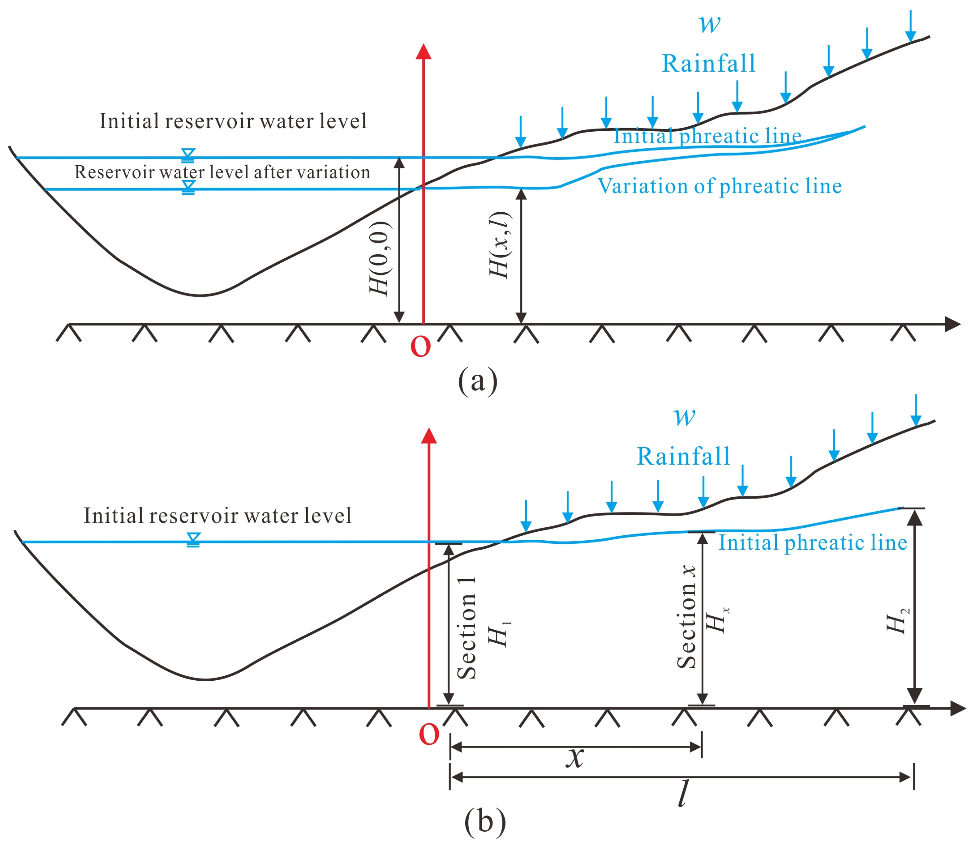
As shown in Figure 1a, the temporal evolution of groundwater levels along the reservoir landslide at time t with a given instance x is:
u ( x , t ) = H ( x , t ) H ( x , 0 ) ,
where H (x, 0) is the initial water level at the x position, which is a fixed value and can be determined via in situ monitoring.
When t = 0:
u ( x , t ) = 0 ,
When x = 0:
u ( 0 , t ) = H ( 0 , t ) H ( 0 , 0 ) = f ( t ) ,
where the variation of the reservoir water level, expressed by the function f (t), is measurable and can be regarded as a known quantity.
Figure 1. Computational framework of phreatic line. (a) Basic calculation model diagram of the phreatic line when the reservoir water level fluctuation, (b) water balance profle of unsteady two-dimensional fow of phreatic water.
Water 16 00375 g001
Therefore, the unstable seepage of groundwater can be described with the following equation:
{ u ( x , 0 ) = 0   ( 0 < x < ) u ( 0 , t ) = f ( t )   ( t > 0 ) u ( , t ) = β t   ( t > 0 ) H t = α 2 H x 2 + β   ( 0 < x < , t > 0 ) ,
where u (∞, t) = βt represents the change of groundwater level at time t with an infinite distance from the origin. It is assumed that the fluctuation of reservoir water level has no effect on the groundwater level in the infinite distance, which is only affected by rainfall infiltration, and the rainfall intensity can be obtained via in situ monitoring.

2.3. Calculation of Differential Equations

2.3.1. The Solution of the Initial Phreatic Line

In order to solve the initial phreatic line under steady state, the Dupuit Assumption is adopted in this study. As shown in Figure 1b, the flow rate at Section 1 and Section 2 is set as q1, and the flow rate at the 1~x is set as q2.
q 1 = K H 2 + H 1 2 H 2 H 1 L q 2 = K H + H 1 2 H H 1 x ,
Based on the principle of water balance, that is, q1 = q2, the water head of x section can be derived:
H ( x , 0 ) = x L ( H 2 2 H 1 2 ) + H 1 2 ,

2.3.2. The Solution of Differential Equation

Equation (7) can be solved by Laplace integral transformation. Both sides of the model equation are multiplied by eat at the same time, and the equation after integral transformation is as follows:
{ u ¯ ( x , 0 ) = 0 u ¯ ( 0 , t ) = F ( a ) u ¯ ( , t ) = β t 2 u ¯ x 2 = u ¯ a α + β a α ,
Assuming u ¯ = 0 + u e a t d t , 0 + f ( t ) d t = F ( t ) , the general solution of the second-order nonhomogeneous differential equation is:
u ¯ = ( F ( a ) β t ) e a α x + β t ,
Equation (11) can be further simplified by taking the inverse Laplace transform:
u = L 1 [ u ¯ ] = ( f ( t ) β t ) L 1 [ e a α x ] + β t ,
L 1 [ e a α λ ] = 4 i 2 e r f c ( λ ) = ( 1 + 2 λ 2 ) e r f c ( λ ) 2 π e λ 2 ,
where e r f c ( λ ) = 2 π λ + e t 2 d t is the residual error function, which can be obtained by looking up the error function table. λ = x 2 α t is the groundwater influence factor. K , h m , μ are constants, λ is a function of x (distance from the origin) and t (duration). λ is positively correlated with x and negatively correlated with t.
R(λ) is the groundwater influence coefficient:
R ( λ ) = L 1 [ e a α λ ] ,
The relationship between λ and R(λ) is illustrated in Figure 2; it can be seen that R(λ) is a decreasing function with the increasing of λ; when λ ≥ 2, R(λ) is approximately equal to 0.
As can be seen from Equation (13), it is very difficult to solve R(λ) directly. Observation of Figure 2 reveals that R(λ) manifests as a continuous and smooth curve. Consequently, the polynomial fitting method is adopted to fit R(λ), and the fitting result is as follows:
R ( λ ) = 0.1091 λ 4 0.750 λ 3 + 1.9283 λ 2 2.2319 λ + 1 ,
By substituting R(λ) into Equation (12), the following equation can be obtained:
u ( x , t ) = ( f ( t ) β t ) R ( λ ) + β t ,
Based on Equations (4) and (16), the ensuing equation is derived:
H ( x , t ) = H ( x , 0 ) ( f ( t ) β t ) R ( λ ) β t ,
By combining Equations (15) and (17), the groundwater level infiltration line calculation expression can be expressed as:
H ( x , t ) = { H ( x , 0 ) ( f ( t ) W μ t ) ( 0.1091 λ 4 0.750 λ 3 + 1.9283 λ 2 2.2319 λ + 1 ) W μ t   ( 0 < λ < 2 ) 0   ( λ 2 )

3. Case Study: Majiagou Landslide

3.1. Regional Geological Setting

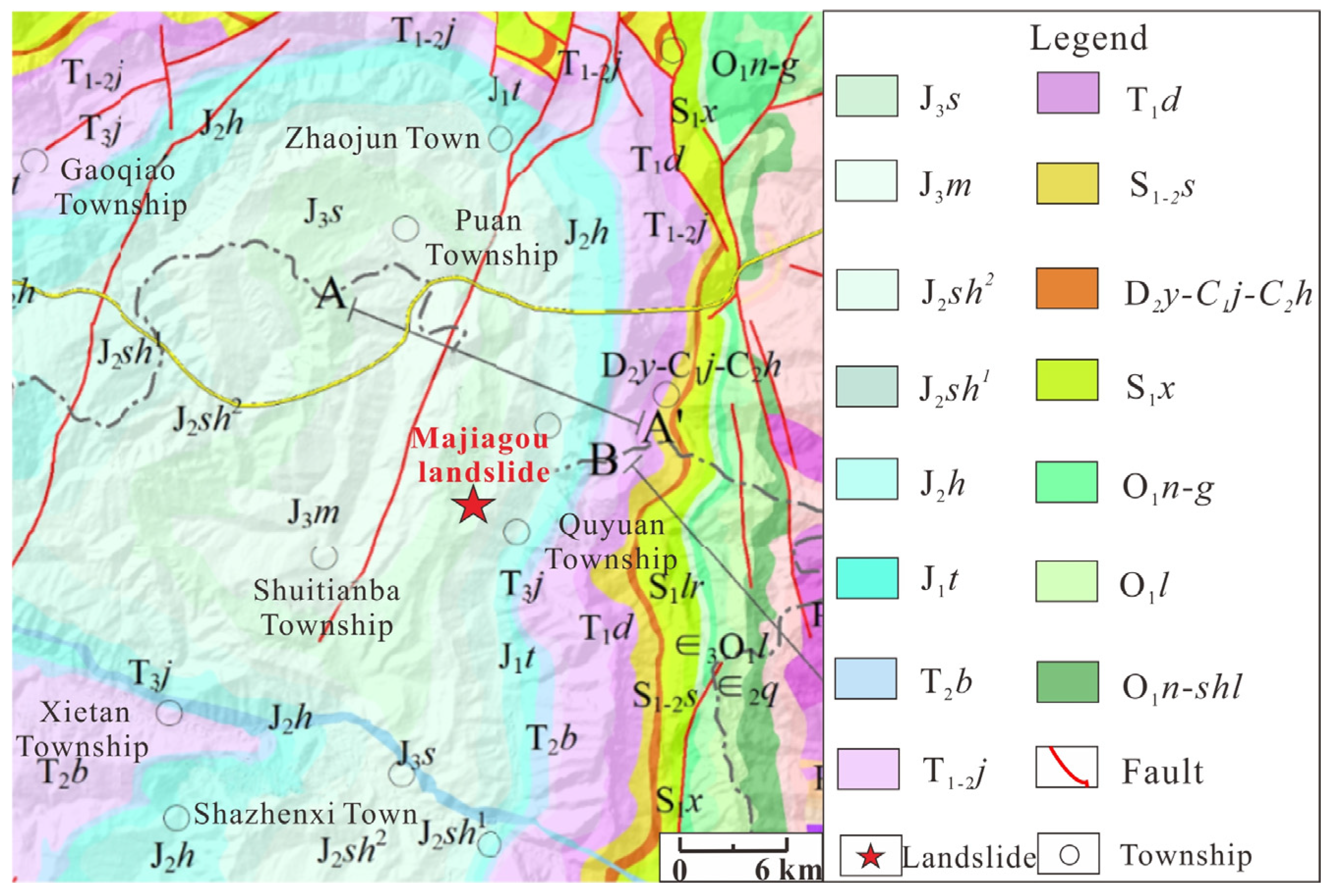
The geological SketchUp map of the study area is illustrated in Figure 3. The regional stratigraphy is well developed, with exposures ranging from the Jurassic to the Ordovician stratum. The main formations around the Majiagou landslide include the Jurassic stratum (Upper Jurassic, Middle Jurassic) and the Quaternary stratum. Within the Jurassic stratum, there are formations such as the Penglai Formation (J2p), the Suining Formation (J2sh2), the Shaximiao Formation (J2sh1), and the Niejiashan Formation (J2n). The Quaternary deposits are sporadically distributed in the study area, including river terraces, various levels of erosion surfaces, slope depressions, etc.
The study area is located on the eastern margin of the Ziguitai fold belt in the Upper Yangtze Platform, mostly within the Zigui Basin. The eastern part extends into the Huangling anticline, which trends in a north–northeast direction. The structural system is situated at the northern end of the Emei uplift zone in the New Cathaysia tectonic system and the composite area of the Huaiyangshan-shaped tectonic system. The folding structures are mainly represented by the nearly north–south trending Zigui syncline, while the fault structures include the north–northeast-oriented compressional Shuitianba fault and the compressional to transpressional Huangjingshuping fault, which are approximately parallel in distribution.

3.2. Engineering Geological Setting of Majiagou Landslide

3.2.1. Location of Majiagou Landslide

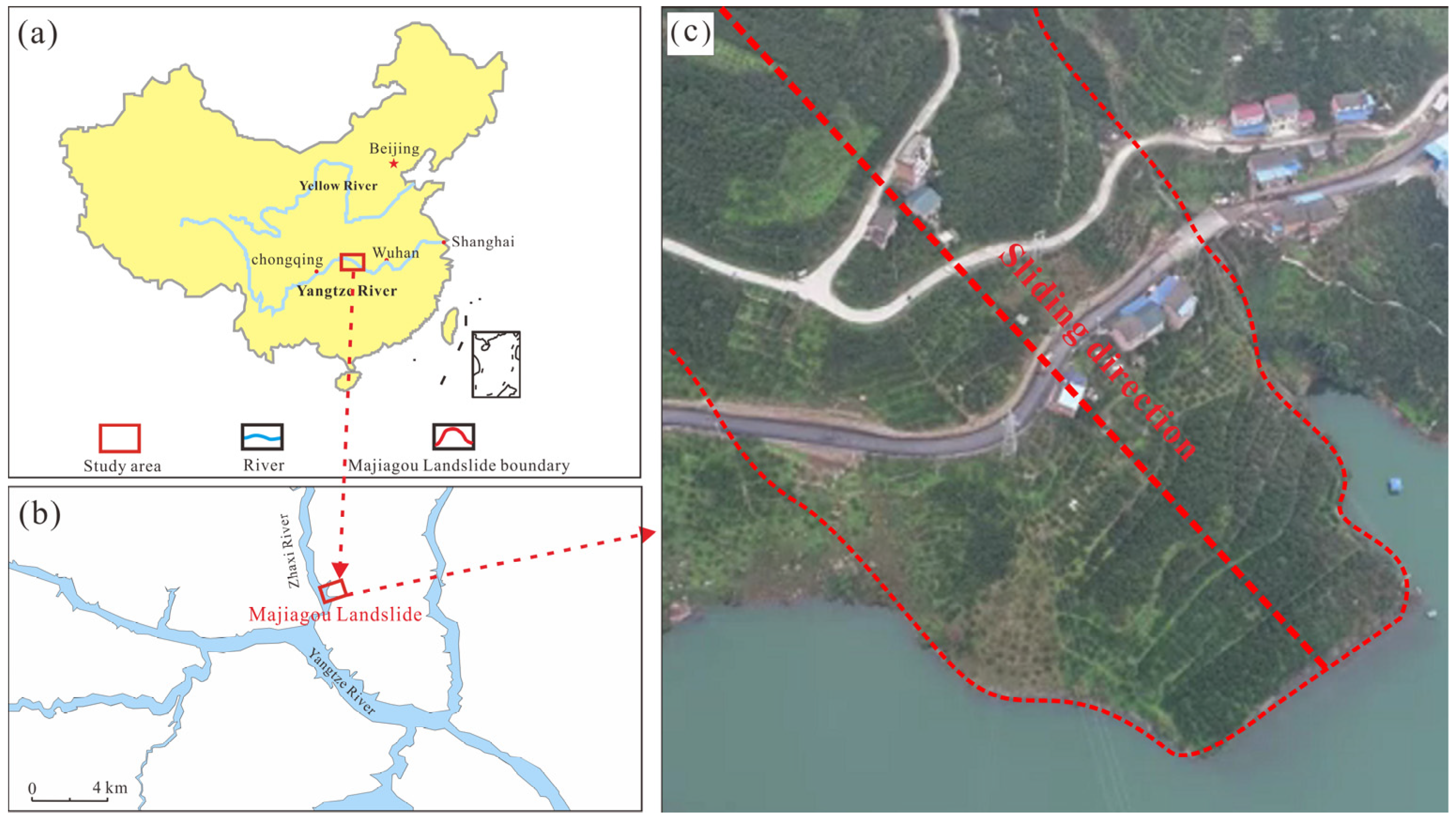
The Majiagou landslide is located in Pengjiapo Village, Guizhou Town, Zigui County, Hubei Province, within the vicinity of TGR area (see Figure 4a,b). It is 2.1 km away from the Yangtze River estuary.

3.2.2. Geomorphological Setting of Majiagou Landslide

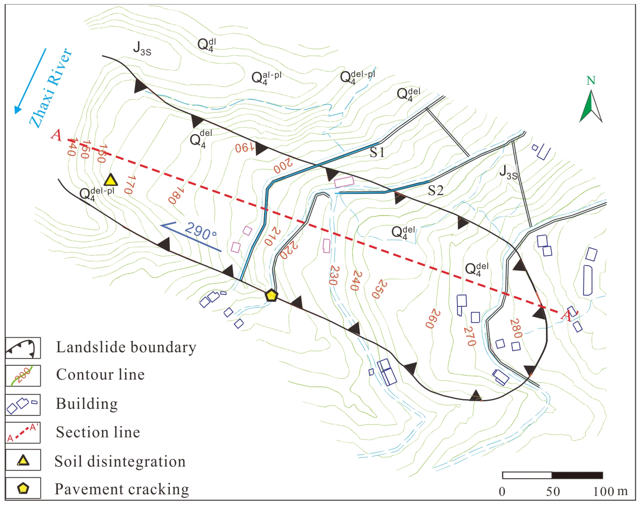
The Majiagou landslide exhibits a configuration characterized by a cohesive tongue-shaped distribution, featuring numerous gently inclined platforms interspersed with steep ridges (Figure 4c). The sliding direction is approximately 290° (Figure 5). The cumulative extent of the slope spans approximately 560 m, with a frontal edge elevation of approximately 125 m and a width of approximately 150 m. In addition, the rear edge is situated at an elevation of about 286 m, accompanied by a width of approximately 210 m. The area of the slope is about 9.8 × 10⁴ m2 (Figure 5), encapsulating a volume of approximately 1.36 × 10⁶ m3. The overall inclination of the slope is approximately 15°.

3.2.3. Stratigraphic Lithology

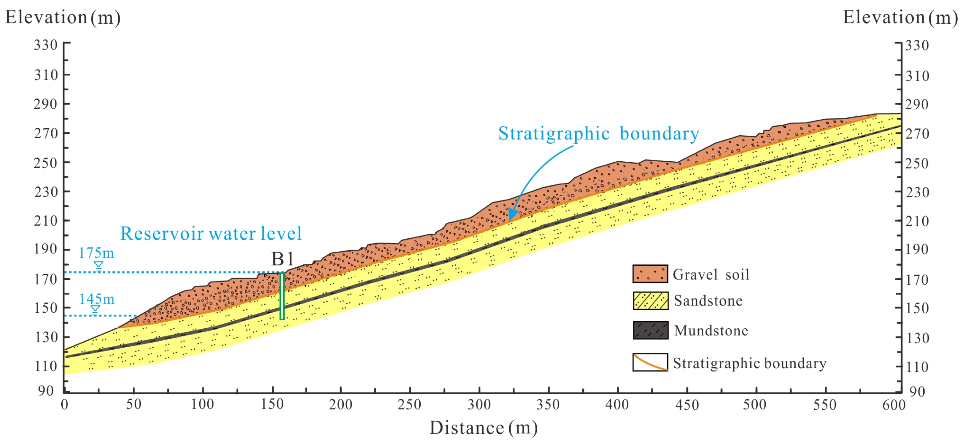
The geological profile of the Majiagou landslide can be characterized into overlying and bedrock strata, delineated in Figure 6. The overlying strata consist of loose accumulations of Quaternary soil, primarily comprised of residual and alluvial soils. The residual soil, constituting a more prevalent occurrence, is characterized by loosely structured gravel soil, exhibiting a thickness ranging from 8 to 15 m. Concurrently, the alluvial soil is widespread on the landslide’s surface, primarily composed of clay with gravel soil. The bedrock stratum is predominantly identified as the Suining Formation (J2sh2), a terrestrial clastic deposition widely distributed in the TGR area. The lithological composition of the rock strata is characterized by gray–white feldspathic quartz sandstone and fine sandstone, interbedded with a thin purple layer of mudstone.

3.3. Monitoring System

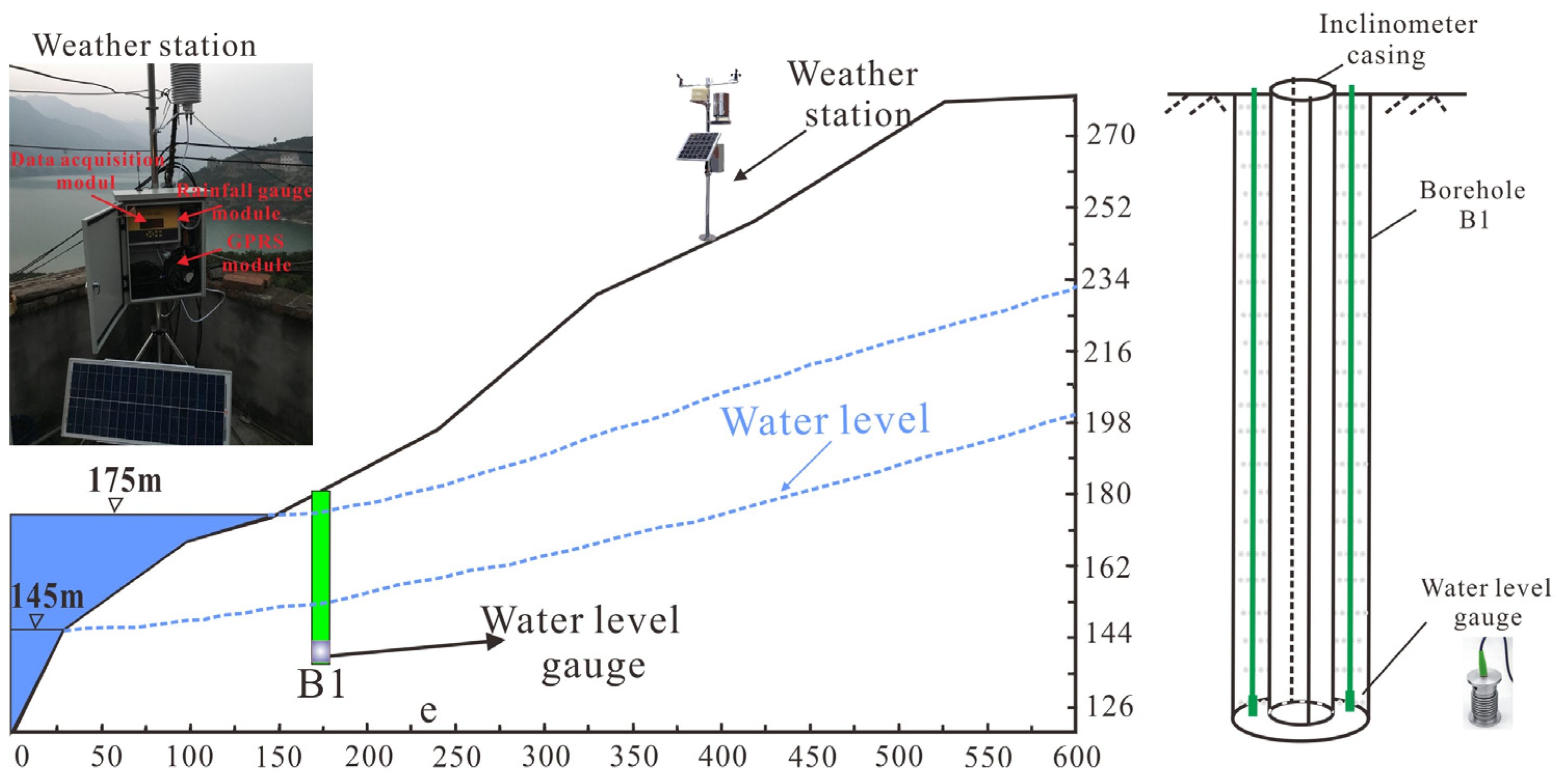
In order to investigate the response of groundwater level to rainfall and reservoir water level fluctuation, a hydrological monitoring station was set up in Majiagou landslide in July 2017. The groundwater level of the landslide could be monitored in real time by installed water level gauges at the bottom of the borehole. In addition, a weather station had been installed on the landslide to record the real-time rainfall data.

3.3.1. Rainfall Monitoring

In order to realize the measurement of Majiagou landslide rainfall, a weather station monitoring system was established in the landslide monitoring center in July 2017 (Figure 7). The station uses a traditional tip-bucket rainfall sensor to measure the amount and intensity of rainfall. The diameter of the rainfall gauge is 200 mm. The measurement accuracy of the sensor is ±4% with a monitoring resolution of 0.1 mm. The monitoring results can be transmitted by a wireless network based on the PH1000 GPRS wireless protocol.

3.3.2. Reservoir Water Level and Groundwater Level Monitoring

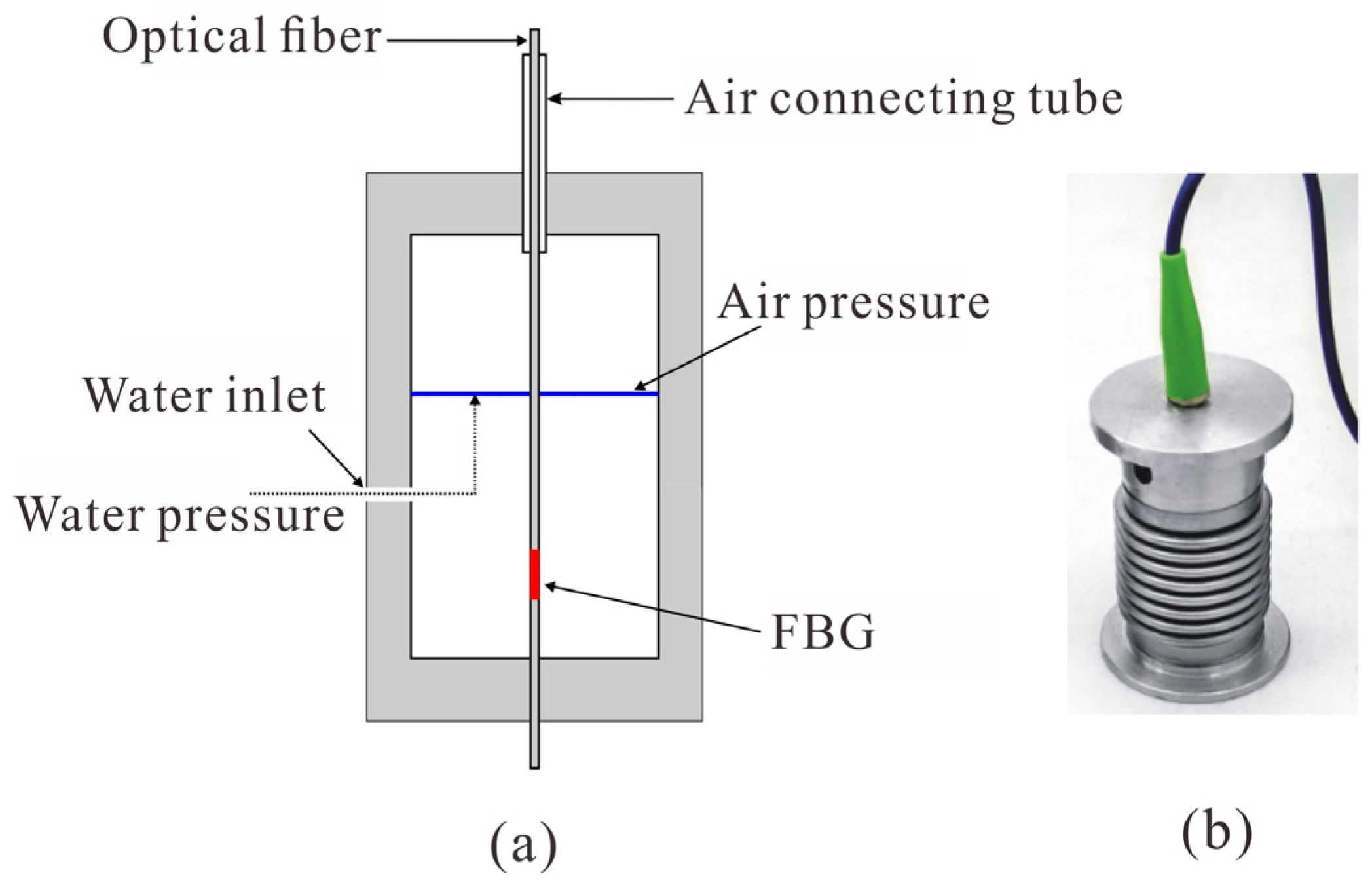
The daily reservoir water level of the Majiagou landslide could be obtained through the website (http://www.xiaoyuka.com/ziguixian/alarm_water/ (accessed on 1 January 2012)), which was released by the Three Gorges hydrology station of the Yangtze River. The groundwater-level fluctuation of the landslide could be recorded by the water level gauges installed in boreholes B1. Figure 8 shows the schematic sketch and physical diagram of the Fiber Bragg Grating (FBG) water level gauge. As shown in Figure 8a, the pressure membrane separates the sensor cavity into two parts: the air pressure cavity and the water pressure cavity. The air pressure chamber is connected to the atmosphere. The monitoring principle of the FBG water level sensor is: the hydrostatic pressure at different water levels will lead to corresponding deformation of the pressure film. By analyzing the deformation of the pressure film, the water level can be determined. It is noted that the water level sensor has a monitoring error of ±1 mm [41].

3.4. Results and Analysis

3.4.1. Rainfall

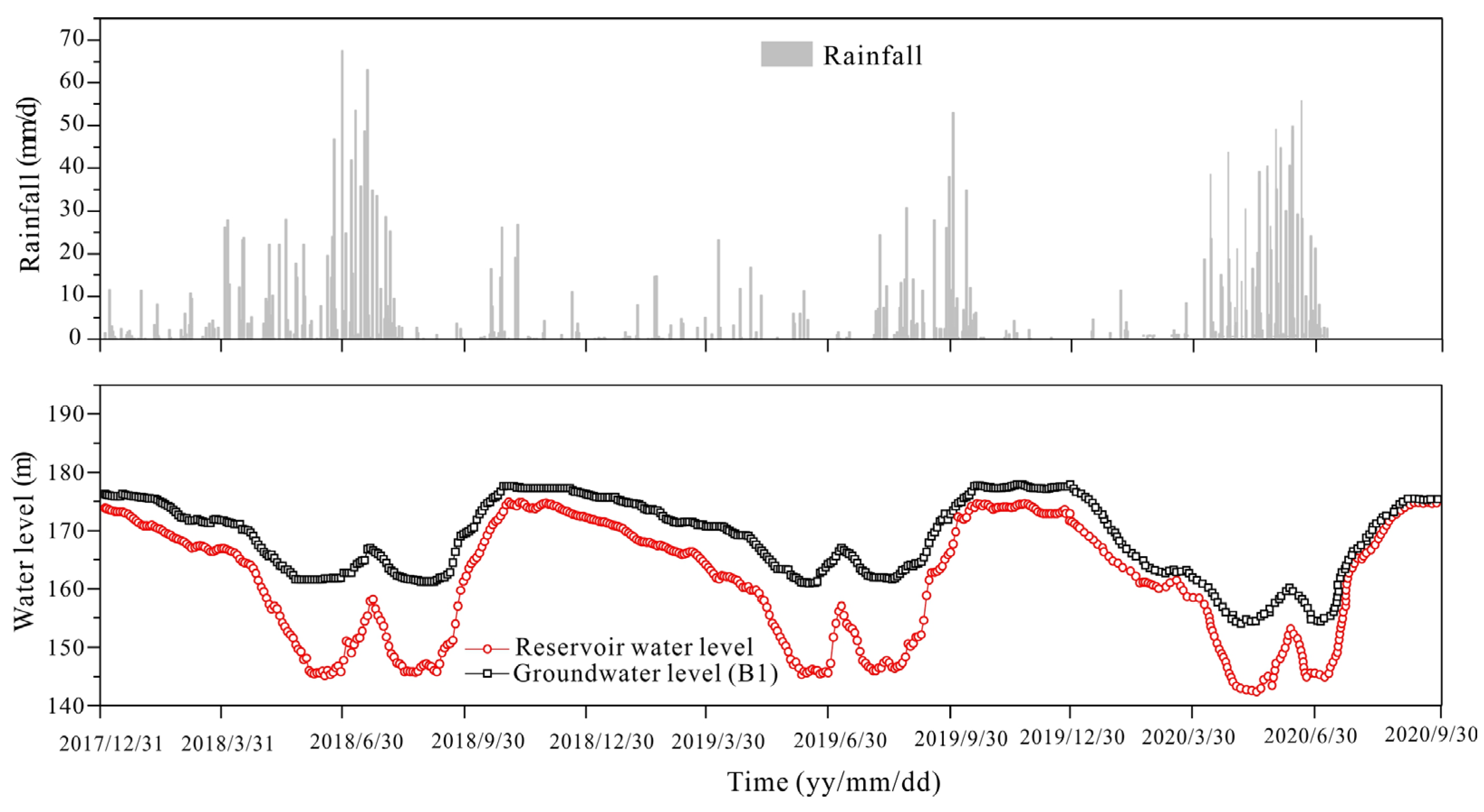
The measured daily rainfall during the period of 2018 to 2020 is shown in Figure 9. The results indicate that rainfall in the Majiagou landslide region was concentrated predominantly between April and August each year, characterized by continuous rainfall with maximum daily precipitation reaching 70 mm. Conversely, from October to March of the following year, rainfall was relatively minimal, with daily precipitation generally below 10 mm, falling within the category of light rain. The rainy season was mostly dominated by heavy or continuous rainfall types. Continuous rainfall generally occurred in Spring and Fall, and daily precipitation exceeding 35 mm mainly occurred in July and August each year. It should be noted that the rainfall during the months of April to August constituted 60–70% of the total annual precipitation.

3.4.2. Fluctuation of Reservoir Water Level and Groundwater Level

The reservoir water level and groundwater level time–history curves for the Majiagou landslide are depicted in Figure 9. Analysis of the reservoir water level variation revealed a distinct cyclic pattern. The reservoir water level attained its peak at 175 m in the Winter season (November) each year. Subsequently, from November to July of the next year, the reservoir underwent a drawdown stage, during which the reservoir water level decreased from the peak at 175 m to the lowest level at 145 m. Notably, the drawdown of the reservoir water level could be divided into two stages: from the Winter season to the Spring season (November to May) of each year, the water level gradually decreased at a rate of 0.19 m/d, followed by a rapid decline at the rate of 0.86 m/d in the Summer season (from May to July). Subsequently, in the Autumn season (from July to September) each year, characterized by concentrated rainfall in the reservoir area, the water level experienced rapid fluctuations but generally maintained a low level. Finally, in the Winter season (from September to November), the reservoir entered a storage phase, with the water level rising from the lowest level of 145 m to the peak of 175 m quickly.
Because the inclinometer B1 is close to the reservoir, and the overlying layer of landslide is mainly permeable gravel soil, the groundwater level variation at inclinometer B1 closely aligned with the reservoir water level fluctuation.

3.5. Model Verification

According to the calculation model of the phreatic line proposed in this study, the parameters that needed to be determined include the thickness hm of the aquifer, the permeability coefficient of the soil/rock of the Majiagou landslide, the gravity water yield μ and the distance x from borehole B1 to the origin. The above-mentioned parameters could be comprehensively determined based on field and laboratory tests as well as inversion analysis, as shown in Table 1 [42]. It should be pointed out that the intersection point between the reservoir water level and the bank slope on the base plate after the reservoir water level drops was set as the origin of coordinates. Thus, in this study, the distance x equaled 110 m. Additionally, in order to simplify the calculations, unsaturated soils were not considered in this study, so the permeability coefficient selected in this study was the saturated permeability coefficient of gravelly soils.
By substituting the parameters listed in Table 1 into Equation (18), the analytical solution of the groundwater level could be obtained, as shown in Figure 10. The red line represented the analytical results and the black dots represented the measured results. It was evident that the groundwater level calculated with the analytical method was slightly higher than the true values. But in general, the change trend and value of the analytical solution were basically the same with those of the measured results.
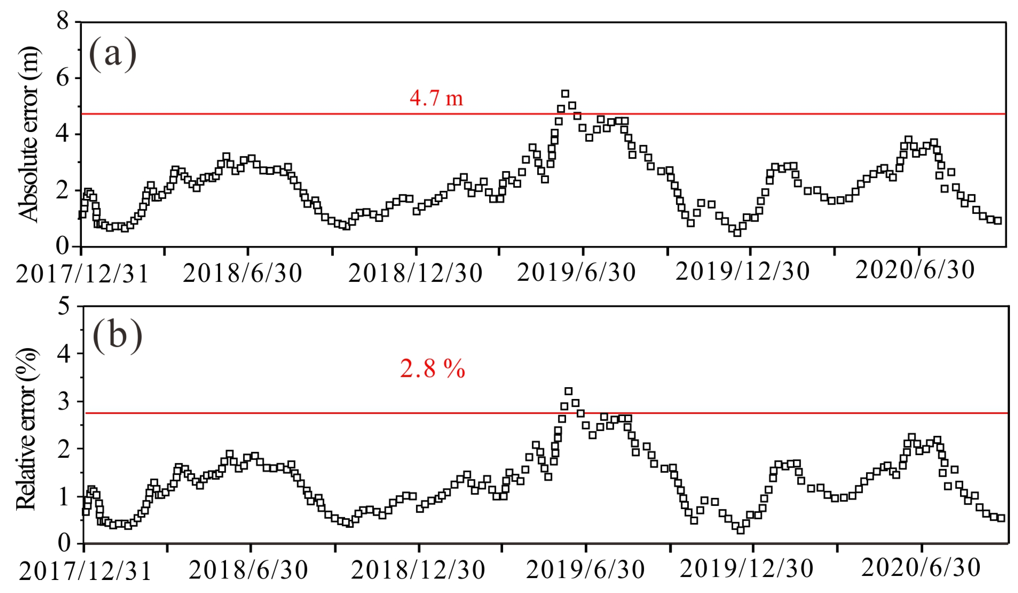
In order to further evaluate the accuracy of the model, we calculated the absolute error and relative error between the analytic values and the measured values, and the results are shown in Figure 11. As can be seen from Figure 11a, when the reservoir water level was at the highest level or dropping slowly, the difference between the analytical results and the measured values was small, basically within the range of 1–2 m. When the reservoir water level decreased rapidly or was at a low level, the difference between the analytical results and measured results was larger, and the maximum error could attain about 4.7 m. This was because the highest reservoir water level was set as the initial moment. In accordance with the assumption articulated in Section 2, denoted as “Prior to the change in reservoir water level, groundwater flow within the reservoir bank slope is assumed to be steady”, the phreatic line obtained in the case of steady seepage was used as the initial value for unsteady seepage flows. Even if the reservoir water level started to drop, due to the low rate of decrease, this led to a small difference between the results calculated by the analytical model and the measured values. However, when the reservoir water level fluctuated rapidly, vertical seepage was generated within the landslide, and the Dupuit Assumption was no longer be satisfied. In this case, the errors between analytical results and measured values become obvious. The error of 4.7 m seems large, but considering that the fluctuation range of the reservoir water level was between 145 m and 175 m, the impact on the result might not be significant. Consequently, to provide a more nuanced assessment, we calculated the relative error as a means of refining the accuracy evaluation. It is evident from Figure 11b that the relative error between analytical results and measured results was basically within 2.8%. In general, the calculation model of the landslide phreatic line proposed in this study is reasonable, and its calculation results could meet the needs of engineering applications.

4. Discussion

4.1. The Innovation of This Study

Groundwater is an important factor affecting the stability of landslides. Therefore, how to accurately calculate the phreatic line is very important in the evaluation and prediction of landslide stability. In recent years, many scholars have adopted numerical analysis methods such as Geo-seep and Moldflow to investigate groundwater seepage variation. Although numerical simulation can obtain accurate and detailed seepage field information of the landslides, it often requires the establishment of an accurate 2D or 3D model, followed by grid division, parameter optimization, and complex calculations. The whole process is time-consuming and often encounters the non-convergence problem, which is not conducive to the rapid analysis and evaluation of landslide stability for engineering purposes. In contrast, the analytical method, based on some assumptions, can quickly derive the exact solution of the phreatic line, which is of great significance for landslide prediction and early warning studies. However, previous analytical methods mainly have two following shortcomings: (1) The bank slope within the water-level fluctuation zone is considered as vertical, which differs significantly from the actual situation. It is noted that the front slope of landslide deposits in the TGR area is generally 10~30°, which is relatively gentle. Given that the fluctuation amplitude of the reservoir water level is 30 m (145 m–175 m), assuming that the front slope is 30°, the length of reservoir bank within the water-level fluctuation zone is 60 m, whereas it is 172.7 m when assuming the front slope is 10°. Therefore, the length of reservoir bank within the water-level fluctuation zone in the TGR area is relatively long, mostly between 60 m and 172.7 m. Thus, the bank slope within the water-level fluctuation zone cannot be regarded as vertical. (2) The fluctuation rate of the reservoir water level is considered as constant. Actually, the fluctuation rate changes with time. To address the above issues, this study carries out an analytical study for the solution of the phreatic line. First, the bank slope within the water level fluctuation zone is considered in terms of its actual geometric inclination rather than assumed to be vertical. This can be corrected according to the actual geologic profile of the landslide. Second, the fluctuation rate of the reservoir water level variation is consistent with the actual situation rather than assumed to be constant. This can be corrected by changing u (0, t) = vt proposed by Wu et al., 2009 [37] and Sun et al., 2017 [39] to u (0, t) = f (t), as depicted in Equation (7) in this study.

4.2. Error Analysis and Limitations of the Proposed Method

Based on the phreatic line calculation model as described in Equation (18), it can be seen that in addition to rainfall and reservoir water level fluctuation, the phreatic line inside the landslide is also affected by the permeability coefficient of rock/soil, gravity water yield, thickness of the aquifer and the horizontal distance of the calculated point to the origin.
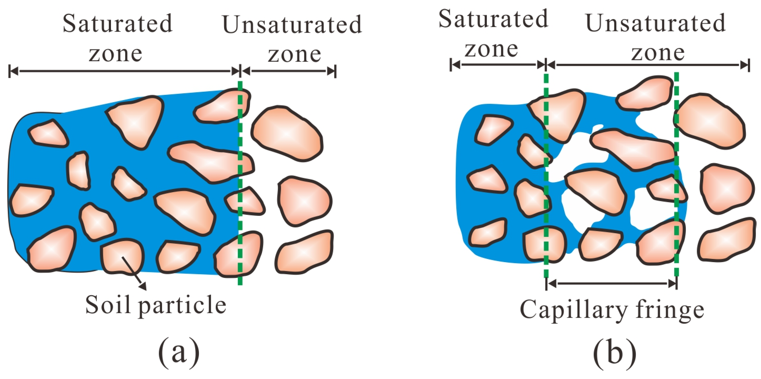
The schematic diagram of groundwater flow within soil is illustrated in Figure 12. In fact, the groundwater flow within the soil should follow the pattern as illustrated in Figure 12b. That is, the groundwater flow considers the soil as a two-layer system consisting of a saturated zone and an unsaturated zone with a capillary fringe. If the capillary fringe is considered, the physical properties of unsaturated soils, including the permeability coefficient and water content, are highly nonlinear [43,44]. At present, there is no analytical solution model that can solve such highly nonlinear equations involved in unsaturated soil. Given this, the groundwater flow is simplified as Figure 12a. That is, the capillary fringe is not considered and the flow of groundwater in soil is considered as saturated seepage. This simplification will lead to an error between the calculated result and the real value.
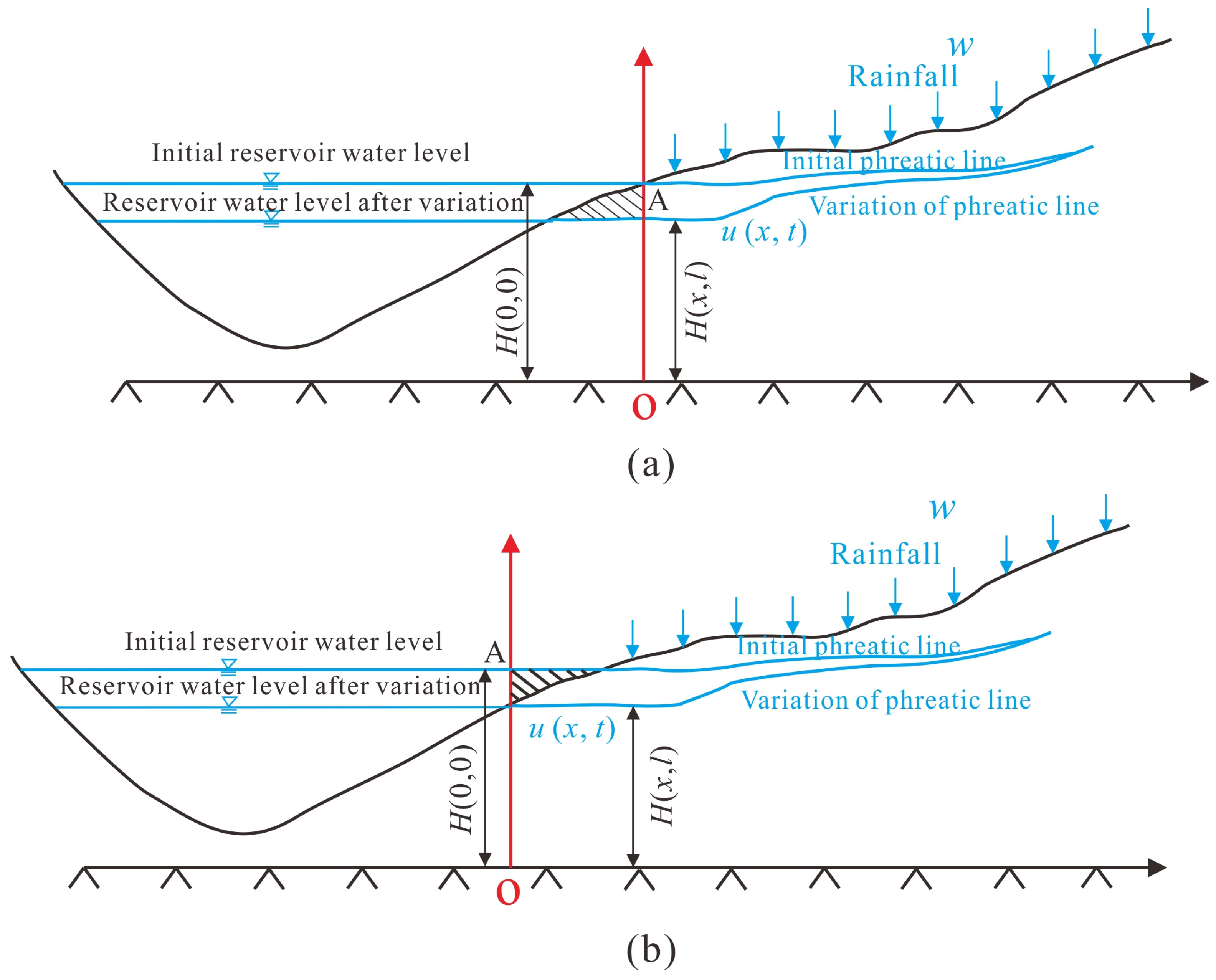
In addition to the error caused by not considering unsaturated soil, the selection of coordinate origin can also induce error. As shown in Figure 13, the phreatic line within the Majiagou landslide is observed to be higher than the measured value. The primary reason is that the position of the origin of coordinates will directly affect the accuracy of the phreatic line calculation result. The first method, as illustrated in Figure 13a, assumes that the projection of the intersection point (marked with “A”) between the reservoir water level and the bank slope on the base plate before the reservoir water level drops is the origin of coordinates. It is evident that this method only calculates the position of the phreatic line from the origin section to the rear edge of the landslide, and ignores the phreatic line in the range of the reservoir water level fluctuation zone, which is marked in shadow in Figure 13a. Consequently, the aforementioned point is precluded from serving as the origin of coordinates in the calculation of the phreatic line within the landslide. Generally, the second method, as illustrated in Figure 13b, assumes that the intersection point (marked with “A”) between the reservoir water level and the bank slope on the base plate after the reservoir water level drops is the origin of coordinates. This method, adopted in this study, is more accurate than the former method in terms of phreatic line calculation. However, the phreatic lines calculated by this method are higher than the actual ones. The main reason is that the shadow part, as illustrated in Figure 13b, should be empty but is treated as soil. This will cause the drawdown of the phreatic line to become slower than the actual situation. Thus, the calculated phreatic line is higher than the measured value.
Generally speaking, considering that the relative error between analytical results and measured results is basically within 2.8%, its calculation results can meet the needs of engineering applications, which demonstrates the feasibility and accuracy of the proposed method.

5. Conclusions

According to the basic equation of unstable diving motion, the unsteady seepage differential equation of landslide groundwater under the coupling effect of reservoir level fluctuation and rainfall is established. Considering the actual bank slope and reservoir water level fluctuation rate, a novel analytical model is proposed. Based on the developed phreatic line calculation model, it is found that in addition to rainfall and reservoir water level fluctuation, the phreatic line inside the landslide is also affected by the permeability coefficient of rock/soil, gravity water yield, thickness of the aquifer and the horizontal distance of the calculated point to the origin. Then, the developed analytical model is applied to the Majiagou landslide in the TGR. When the reservoir water level is at the high level or drops slowly, the difference between the analytical results and the measured values is small, basically within the range of 1–2 m. In contrast, when the reservoir water level decreases rapidly or is at the low level, the difference between the analytical results and measured results is larger, and the maximum error can attain about 4.7 m. The source of the error can be divided into two aspects. First, in order to simplify the calculations, the unsaturated case is not considered in this study, which means that the flow of groundwater in the soil is considered as saturated seepage. Second, the coordinate origin is set as the intersection of the reservoir level and the bank slope on the bottom plate after the reservoir level drops. That is, the water level fluctuation zone should be empty but is treated as soil. But generally, the relative error between the analytical results and the measured results is basically within 2.8%; the calculation results can, therefore, meet the needs of engineering applications. This study provides an effective and accurate landslide phreatic line calculation method, which is of great significance for landslide prediction and early warning.

Author Contributions

L.Z. and H.H. proposed the idea and designed the framework of this paper; C.M., J.Y. and J.W. collected the data; L.Z., C.M., J.Y. and H.H. completed the analyses and summary of the results; L.Z. wrote the paper; H.H. polished the language and provided some suggestions on the organization of this paper. All authors have read and agreed to the published version of the manuscript.

Funding

The authors gratefully acknowledge the financial support provided by the Fundamental Research Funds for the Central Universities (2-9-2022-042). Opening fund of State Key Laboratory of Geohazard Prevention and Geo-environment Protection (SKLGP2023K021), Technology Innovation Center for Geohazard Monitoring and Risk Early Warning (TICGM-2023-04) and Key Laboratory of the Ministry of Education for Geomechanics and Embankment Engineering, Hohai University (2023002).

Data Availability Statement

Data are contained within the article.

Acknowledgments

The authors would like to thank Guozhong Tang, Jiahao Wang and Jiaying Yang for their assistance in format revision.

Conflicts of Interest

The authors declare no conflicts of interest.

References

  1. Tang, H.M.; Wasowski, J.; Juang, C.H. Geohazards in the three Gorges Reservoir Area, China- Lessons learned from decades of research. Eng. Geol. 2019, 261, 105267. [Google Scholar] [CrossRef]
  2. Lin, P.; Liu, X.; Zhang, J. The simulation of a landslide-induced surge wave and its overtopping of a dam using a coupled ISPH model. Eng. Appl. Comp. Fluid. 2015, 9, 432–444. [Google Scholar] [CrossRef]
  3. Tan, H.; Chen, S. A hybrid DEM-SPH model for deformable landslide and its generated surge waves. Adv. Water Resour. 2017, 108, 256–276. [Google Scholar] [CrossRef]
  4. Zhang, L.; Shi, B.; Zhang, D.; Sun, Y.J.; Inyang, H.I. Kinematics, triggers and mechanism of Majiagou landslide based on FBG real-time monitoring. Environ. Earth Sci. 2020, 79, 200. [Google Scholar] [CrossRef]
  5. Zhang, L.; Zhu, H.; Han, H.; Shi, B. Fiber optic monitoring of an anti-slide pile in a retrogressive landslide. J. Rock Mech. Geotech. Eng. 2023, 16, 333–343. [Google Scholar] [CrossRef]
  6. Zhang, L.; Cui, Y.; Zhu, H.; Wu, H.; Han, H.; Yan, Y.; Shi, B. Shear deformation calculation of landslide using distributed strain sensing technology considering the coupling effect. Landslides 2023, 20, 1583–1597. [Google Scholar] [CrossRef]
  7. Genevois, R.; Tecca, P.R. The Vajont landslide: State-of-the-art. Ital. J. Eng. Geol. Environ. 2013, 15–39. [Google Scholar] [CrossRef]
  8. Wolter, A.; Stead, D.; Clague, J.J. A morphologic characterisation of the 1963 Vajont Slide, Italy, using long-range terrestrial photogrammetry. Geomorphology 2014, 206, 147–164. [Google Scholar] [CrossRef]
  9. Boon, C.W.; Houlsby, G.T.; Utili, S. New insights into the 1963 vajont slide using 2D and 3D distinct-element method analyses. Géotechnique. 2014, 64, 800–816. [Google Scholar] [CrossRef]
  10. Ibañez, J.P.; Hatzor, Y.H. Rapid sliding and friction degradation: Lessons from the catastrophic Vajont landslide. Eng. Geol. 2018, 244, 96–106. [Google Scholar] [CrossRef]
  11. Jian, W.; Xu, Q.; Yang, H.; Wang, F. Mechanism and failure process of Qianjiangping landslide in the Three Gorges Reservoir, China. Environ. Earth Sci. 2014, 72, 2999–3013. [Google Scholar] [CrossRef]
  12. Yin, Y.P.; Huang, B.; Chen, X.; Liu, G.; Wang, S. Numerical analysis on wave generated by the Qianjiangping landslide in Three Gorges Reservoir, China. Landslides 2015, 12, 355–364. [Google Scholar] [CrossRef]
  13. Ma, J.; Tang, H.; Hu, X.; Bobet, A.; Zhang, M.; Zhu, T.; Song, Y.; Ez Eldin, M.A.M. Identification of causal factors for the Majiagou landslide using modern data mining methods. Landslides 2017, 14, 311–322. [Google Scholar] [CrossRef]
  14. Zhang, L.; Shi, B.; Zhu, H.; Yu, X.B.; Han, H.; Fan, X. PSO-SVM-based deep displacement prediction of Majiagou landslide considering the deformation hysteresis effect. Landslides 2021, 18, 179–193. [Google Scholar] [CrossRef]
  15. Zhang, L.; Shi, B.; Zhu, H.; Yu, X.; Wei, G. A machine learning method for inclinometer lateral deflection calculation based on distributed strain sensing technology. Bull. Eng. Geol. Environ. 2020, 79, 3383–3401. [Google Scholar] [CrossRef]
  16. Ye, X.; Zhu, H.H.; Wang, J.; Zhang, Q.; Shi, B.; Schenato, L.; Pasuto, A. Subsurface multi-physical monitoring of a reservoir landslide with the fiber-optic nerve system. Geophys. Res. Lett. 2022, 49, e2022GL098211. [Google Scholar] [CrossRef]
  17. Han, H.; Shi, B.; Zhang, L. Prediction of landslide sharp increase displacement by SVM with considering hysteresis of groundwater change. Eng. Geol. 2021, 280, 105876. [Google Scholar] [CrossRef]
  18. Kafle, L.; Xu, W.J.; Zeng, S.Y.; Nagel, T. A numerical investigation of slope stability influenced by the combined effects of reservoir water level fluctuations and precipitation: A case study of the Bianjiazhai landslide in China. Eng. Geol. 2022, 297, 106508. [Google Scholar] [CrossRef]
  19. Yang, B.; Yin, K.; Xiao, T.; Chen, L.; Du, J. Annual variation of landslide stability under the effect of water level fluctuation and rainfall in the Three Gorges Reservoir, China. Environ. Earth Sci. 2017, 76, 564. [Google Scholar] [CrossRef]
  20. Huang, F.; Luo, X.; Liu, W. Stability analysis of hydrodynamic pressure landslides with different permeability coefficients affected by reservoir water level fluctuations and rainstorms. Water 2017, 9, 450. [Google Scholar] [CrossRef]
  21. Hou, T.S.; Xu, G.L.; Zhang, D.Q.; Liu, H.Y. Stability analysis of Gongjiacun landslide in the three Gorges Reservoir area under the action of reservoir water level fluctuation and rainfall. Nat. Hazards 2022, 114, 1647–1683. [Google Scholar] [CrossRef]
  22. Yan, Y.; Cui, Y.F.; Huang, X.H.; Zhou, J.J.; Zhang, W.G.; Yin, S.Y.; Guo, J.; Hu, S. Combining seismic signal dynamic inversion and numerical modeling improves landslide process reconstruction. Earth Surf. Dyn. 2022, 10, 1233–1252. [Google Scholar] [CrossRef]
  23. Yan, Y.; Tang, H.; Hu, K.H.; Turowski, J.M.; Wei, F.Q. Deriving debris-flow dynamics from real-time impact-force measurements. J. Geophys. Res.-Earth Surf. 2023, 128, e2022JF006715. [Google Scholar] [CrossRef]
  24. Nie, J.Y.; Cui, Y.; Wu, Z.; Zhang, L.; Fang, J. DEM study on role of fines in mobility of dry granular flows considering particle size-shape correlation. Comput. Geotech. 2024, 166, 105980. [Google Scholar] [CrossRef]
  25. Nie, J.Y.; Cui, Y.; Wang, G.; Wang, R.; Zhang, N.; Zhang, L.; Wu, Z. A comprehensive numerical investigation of multi-scale particle shape effects on small strain stiffness of sands. Géotechnique 2024, 74, 1–12. [Google Scholar]
  26. Ye, X.; Zhu, H.; Cheng, G.; Pei, H.; Shi, B.; Schenato, L.; Pasuto, A. Thermo-hydro-poro-mechanical responses of a reservoir-induced landslide tracked by high-resolution fiber optic sensing nerves. J. Rock Mech. Geotech. Eng. 2024, in press. [CrossRef]
  27. Yan, Z.L.; Wang, J.J.; Chai, H.J. Influence of water level fluctuation on phreatic line in silty soil model slope. Eng. Geol. 2010, 113, 90–98. [Google Scholar] [CrossRef]
  28. Huang, G.H.; Wang, H.; Adoko, A.C. Dam phreatic line simulation on FLAC3D: A case study. Appl. Mech. Mater. 2023, 353, 407–410. [Google Scholar]
  29. Yang, H.; Tang, M.; Xu, Q.; Xiao, X.; Li, H. Modification of phreatic line calculation model for landslide accumulation in the Three Gorges Reservoir area. Bull. Eng. Geol. Environ. 2022, 81, 175. [Google Scholar] [CrossRef]
  30. Cheng, L.; Zhang, A.; Cao, B.; Yang, J.; Hu, L.; Li, Y. An experimental study on monitoring the phreatic line of an embankment dam based on temperature detection by OFDR. Opt. Fiber Technol. 2021, 63, 102510. [Google Scholar] [CrossRef]
  31. Zhang, C.; Chai, J.; Cao, J.; Xu, Z.; Qin, Y.; Lv, Z. Numerical simulation of seepage and stability of tailings dams: A case study in Lixi, China. Water 2020, 12, 742. [Google Scholar] [CrossRef]
  32. Sun, Y.; Yang, K.; Hu, R.; Wang, G.; Lv, J. Model test and numerical simulation of slope instability process induced by rainfall. Water 2022, 14, 3997. [Google Scholar] [CrossRef]
  33. Xiong, X.; Matsumoto, T.; Shi, Z.; Zhang, F. Flume tests and corresponding numerical simulation of hydraulic/mechanical behavior of Tangjiashan landslide dam subjected to seepage loading. Soils Found. 2022, 62, 101200. [Google Scholar] [CrossRef]
  34. Jaswal, M.; Sinha, R.K.; Sen, P. Delineation of phreatic surface in soil type slope—A comparative study using physical and numerical modeling. J. Min. Sci. 2020, 56, 494–504. [Google Scholar] [CrossRef]
  35. Zheng, Y.R.; Shi, W.M.; Kong, W.X. Calculation of seepage force and groundwater wetting line when reservoir water level drops. Chin. J. Rock Mech. Eng. 2004, 18, 3203–3210. [Google Scholar]
  36. Wu, Q.; Lin, Z.H. Analytical Solution of the Wet Line in the Layer Bank Slope when the Reservoir Water Level drops. Geol. Sci. Technol. 2007, 2, 91–94. [Google Scholar]
  37. Wu, Q.; Tang, H.M.; Wang, L.Q.; Lin, Z.H. Study on the wetting line of reservoir bank slope under the action of water level rise and fall combined with rainfall. Rock Soil Mech. 2009, 30, 3025–3031. [Google Scholar]
  38. Sun, G.; Lin, S.; Jiang, W.; Yang, Y. A simplified solution for calculating the phreatic line and slope stability during a sudden drawdown of the reservoir water level. Geofluids 2018, 2018, 1859285. [Google Scholar] [CrossRef]
  39. Sun, G.; Yang, Y.; Cheng, S.; Zheng, H. Phreatic line calculation and stability analysis of slopes under the combined effect of reservoir water level fluctuations and rainfall. Can. Geotech. J. 2017, 54, 631–645. [Google Scholar] [CrossRef]
  40. Hua, S.; Li, Y.A.; Zhao, B.B.; Wang, Y.W.; Hu, Y.; Xiao, J.F. Analytical Solutions for Phreatic Line in Bank Slope Under the Combined Effect of Rainfall and Reservoir Water Level Fluctuation. Electron. J. Geotech. 2015, 20, 1439–1448. [Google Scholar]
  41. Sun, Y.J.; Zhang, D.; Shi, B.; Tong, H.J.; Wei, G.Q.; Wang, X. Distributed acquisition, characterization and process analysis of multi-field information in slopes. Eng. Geol. 2014, 182, 49–62. [Google Scholar] [CrossRef]
  42. Zhang, Y.M. Multifield Characteristics and Evolution Mechanism of Majiagou Landslide-Stabilizing Piles System under Reservoir Operations. Doctoral Dissertation, China University of Geoscience (Wuhan), Wuhan, China, 2018. (In Chinese with English abstract). [Google Scholar]
  43. Chan, A.H.C.; Pastor, M.; Schrefler, B.A.; Siomi, T.; Zienkiewicz, O.C. Computational Geomechanics, Theory and Applications, 2nd ed.; Wiley: New York, NY, USA, 2022. [Google Scholar]
  44. Gardner, W.R. Some steady-state solutions of the unsaturated moisture flow equation with application to evaporation from a water table. Soil Sci. 1958, 85, 228–232. [Google Scholar] [CrossRef]
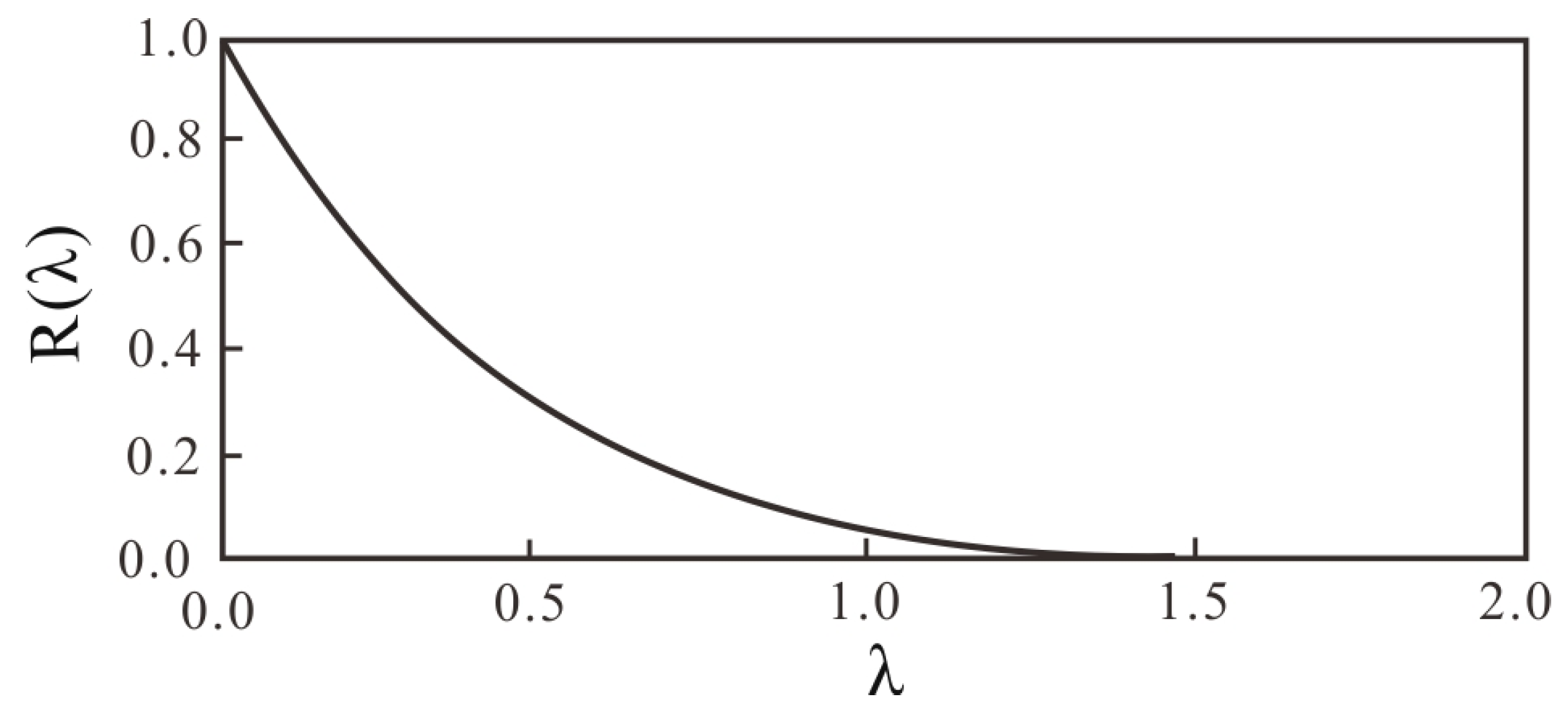
Figure 2. The relation curve of λ and R(λ).
Water 16 00375 g002
Figure 3. The geological SketchUp map of the study area.
Water 16 00375 g003
Figure 4. Location of Majiagou landslide. (a) Location in China. (b) Location in TGR. (c) Aerial view of Majiagou landslide.
Water 16 00375 g004
Figure 5. Topographic map of the Majiagou landslide.
Water 16 00375 g005
Figure 6. Geological profile of Majiagou landslide.
Water 16 00375 g006
Figure 7. Hydrological monitoring station of Majiagou landslide.
Water 16 00375 g007
Figure 8. (a) Schematic diagram of water level gauge. (b) Physical diagram of the water level gauges.
Water 16 00375 g008
Figure 9. Time–history curve of rainfall, reservoir water level fluctuation and groundwater level change.
Water 16 00375 g009
Figure 10. Comparison of daily groundwater between measured and analytical results.
Water 16 00375 g010
Figure 11. Error between analytical and monitoring results. (a) Absolute error. (b) Relative error.
Water 16 00375 g011
Figure 12. Schematic diagram of groundwater flow. (a) The groundwater flow considers the soil as a two-layer system consisting of a saturated zone and unsaturated zone. (b) The groundwater flow considers the soil as a two-layer system consisting of a saturated zone and an unsaturated zone with a capillary fringe above the water table.
Water 16 00375 g012
Figure 13. Error analysis. (a) The origin of coordinates is the intersection point between the reservoir water level and the bank slope on the base plate before the reservoir water level drops. (b) The origin of coordinates is the intersection point between the reservoir water level and the bank slope on the base plate after the reservoir water level drops.
Water 16 00375 g013
Table 1. The parameters of Majiagou landslide.
Gravity Water Yield μThickness of the Aquifer hm (m)Permeability Coefficient K (cm/s)The Distance x (m)
Sliding body0.082151.17 × 10−2110
Sliding bed/6.43 × 10−4
Disclaimer/Publisher’s Note: The statements, opinions and data contained in all publications are solely those of the individual author(s) and contributor(s) and not of MDPI and/or the editor(s). MDPI and/or the editor(s) disclaim responsibility for any injury to people or property resulting from any ideas, methods, instructions or products referred to in the content.