Abstract
In this work, we present a comprehensive extension of the Surface–Underground–Recharge (SUR) water supply model through the incorporation of generalized conformable derivatives. This operator enables the capture of more exotic dynamics within the system, enhancing the modeling framework’s ability to simulate complex hydrological interactions. Additionally, we extend the results to the restricted phase spaces of the analyzed dynamical systems, facilitating a deeper qualitative analysis. To achieve this, we augment the dimension of the generalized conformable SUR system, rendering it an autonomous higher-order system. Furthermore, we introduce a novel conformable function, referred to as the generalized linear conformable combination function, which significantly broadens the scope of our modeling capabilities. Thus, this study contributes to the advancement of hydrological modeling, providing a robust tool for analyzing intricate water resource dynamics in specific regions.
1. Introduction
In recent years, global challenges related to water supply and hydrological sustainability have led to the development of several prominent models for hydrological and water supply management. Models such as the Soil and Water Assessment Tool (SWAT), Hydrologic Modeling System (HMS), and others have become essential in assessing water resources, predicting flow patterns, and aiding in the planning of sustainable water usage across diverse regions. While these models are powerful and widely applied, they often simplify hydrological dynamics by relying on linear approximations or first-order derivatives, which may limit their accuracy in capturing the nonlinear and complex nature of real-world hydrological systems. In this study, we aim to address these limitations by advancing a generalized model that integrates conformable derivatives, enhancing the representation of nonlinear dynamics in water resource modeling. This approach not only increases the flexibility of the model but also improves its applicability across varied hydrological scenarios [1,2,3].
The Supply Water Resource (SUR) model has proven to be a valuable tool for the management and planning of water resources in Mexico. Its ability to analyze and predict water flow behavior based on key factors is crucial for decision-making aimed at ensuring the sustainable use of this vital resource. However, the current formulations of the model exhibit certain limitations in representing the inherent complexity of hydrological systems [4].
The SUR model is fundamentally based on mass balance equations across three primary water supply sources: surface water, groundwater, and recharge. These balances are framed through the theoretical interaction of these three sources, reflecting the dynamic exchanges that occur between them. The conceptualization and assumptions underlying this model are detailed in [4], which provides a comprehensive framework for the theoretical foundations of the model. This approach allows for a better understanding of the interconnections between different water sources, ensuring more accurate predictions and efficient water management strategies.
An important characteristic of the SUR model formulation is the assumption of first-order derivatives in the underlying hydrological processes [4]. While this simplification is advantageous for modeling linear or approximately linear systems, it may not adequately capture the diverse range of behaviors observed in nature. Non-conventional derivatives, such as generalized conformable derivatives, play a crucial role in modeling nonlinear processes [5], including hydrological phenomena, and in representing more intricate dynamics, such as saturation effects and accumulation.
In this paper, we address this limitation by conducting an in-depth exploration of a generalization of the SUR model. Our proposal involves incorporating generalized conformable derivatives within the SUR framework. These derivatives provide a powerful tool to capture nonlinearities and more complex relationships among variables, thereby enhancing the model’s capacity to accurately describe water flow behavior across different scenarios.
We present the mathematical formulation of this extended model and discuss how its inclusion can facilitate a more realistic and flexible representation of hydrodynamic dynamics in the presence of nonlinearities and additional factors. Furthermore, we emphasize the applicability of this approach in multiple scenarios, ranging from watershed assessments to the planning of water resource management in both urban and rural areas. Through this generalization, we aim to provide a more versatile and precise tool for tackling the challenges of water management in diverse and changing contexts.
Many existing programs for groundwater management, such as those in [6,7,8], employ advanced modules and detailed data requirements to model water supply, groundwater flow, and catchment dynamics. For example, tools like PyCHAMP [7] integrate a comprehensive range of socio-environmental factors in agro-hydrological simulations, while WaterpyBal [8] emphasizes a modular approach to water balance modeling that calculates various water budget parameters with high data precision and detailed input from spatial/temporal data. Similarly, ref. [6] explores enhanced information systems (EISs) as an essential foundation for groundwater management in Mediterranean regions. These tools provide detailed insight but require significant time and technical knowledge for setup and use, often limiting accessibility for practical, real-time decision-making.
In contrast, the SUR model presents a streamlined alternative by reducing data complexity and relying on fewer parameters in a time-series format to predict water flow behaviors. Unlike the black-box nature of some comprehensive software solutions, the mathematical simplicity of SUR allows users to implement it with direct algorithms like Runge–Kutta without high computational demands. This reduction in complexity not only makes the model more accessible to users with limited technical resources but also enables a clear focus on core groundwater dynamics without overemphasizing peripheral factors. This adaptability makes SUR a valuable option for capturing essential system behavior effectively, supporting sustainable water management in varied scenarios.
Our research addresses the following questions: How does the incorporation of conformable derivatives affect the predictive capability and robustness of the SUR model in simulating complex hydrological dynamics? Can this generalized model serve as a reliable tool for various water management applications, and how does it compare to established models under different conditions?
Strategic Models for Managing Water Resources
Water supply is essential for sustainability and quality of life in both urban and rural areas. Effective management requires understanding water source dynamics and meeting growing potable water demands. Mathematical models based on mass balance equations have significantly advanced efforts to address these challenges [9,10]. Integrating surface, groundwater, and recharge sources is vital for accurate assessments of water availability and better responses to climatic extremes [11]. Groundwater models, employing aquifer flow equations, are especially crucial in areas with high extraction rates, predicting levels and quality to ensure sustainable use [12].
Existing mathematical models have been instrumental in advancing our understanding of hydrological systems. For instance, ref. [13] emphasizes the importance of multi-scale simulations to analyze surface water and groundwater interactions, though challenges such as data scarcity and uncertainties in hydraulic parameters remain significant barriers. Similarly, ref. [14] demonstrates the effectiveness of three-dimensional modeling for groundwater recharge in different climatic and geographical settings, providing insights into aquifer dynamics. In another study, ref. [15] explores the impacts of aquifer heterogeneity on groundwater flow within riparian zones, employing semi-analytical solutions to model hydraulic conductivity and discharge patterns. Additionally, ref. [16] presents a mathematical framework to predict radon concentrations in artificial aquifers under various recharge and discharge conditions, showcasing its utility as a tracer for hydrological processes. While these models contribute significantly to their respective domains, they often focus on specific aspects, such as groundwater dynamics or surface water interactions, without fully integrating multiple water sources. The SUR model, in contrast, offers a novel approach by deterministically coupling surface water, groundwater, and recharge sources into a unified framework, thus providing a comprehensive tool for assessing water resource availability in diverse scenarios.
The management of water supply relies heavily on the integration of surface and groundwater sources, as this synergy enables a more holistic assessment of water availability and improves responses to challenges such as droughts and floods. Numerous studies have emphasized the importance of coupling these sources to enhance water resource management strategies. For instance, models utilizing advanced computational tools, such as the EPA EPANET software computer program distributed by US EPA have been employed to analyze small-scale water supply networks, providing valuable insights into network efficiency and operations [17].
Innovative frameworks such as Digital Twins (DTs) optimize water distribution by enabling real-time monitoring and predictive maintenance. Their successful application in Valencia, Spain, illustrates their potential to enhance water management [18]. Integrated approaches like the Nexus Water–Food–Energy framework also address interconnected resource challenges, with strategies like improved irrigation and optimized crop patterns proving effective for water sustainability [19].
Understanding surface–groundwater interactions is another key area of research. Coupling strategies such as fully coupled and loosely coupled techniques enable accurate simulations of these dynamics, improving hydrological modeling at multiple scales [20]. Practical methodologies like Integrated Water Resources Management (IWRM) further promote stakeholder collaboration, offering adaptable solutions for sustainable resource management [21]. Enhanced models, such as the analytical hyporheic flux model (AHF), improve predictions of groundwater–surface water interactions, as demonstrated in the Biebrza River case study [22]. Additionally, Big Data analytics and IoT technologies, including smart meters and sensors, provide real-time insights to optimize water use and quality while reducing environmental impacts [23].
The Simplified Unified Resource (SUR) model distinguishes itself by integrating surface water, groundwater, and recharge sources through differential equations and classical computational methods. Its simplicity and minimal variable requirements eliminate the need for specialized software, making it a practical tool for semi-arid regions. Additionally, the inclusion of fractional derivatives allows for more precise modeling by providing an infinite range of values, enhancing the model’s flexibility and accuracy.
Effective water resource management is a matter of global importance, with researchers and scientists worldwide contributing valuable insights into this field. This work specifically continues prior research focused on water supply management in the semi-arid region of Pachuca de Soto, Hidalgo, where this model was applied. Pachuca is recognized as a semi-dry area, as documented in [24]. The current study builds on the methods and findings presented in [4], aiming to refine and extend the understanding of water dynamics in this challenging climate zone.
In summary, recent advancements in water management integrate surface and groundwater systems, innovative computational tools, and dynamic frameworks. The SUR model exemplifies these developments, offering a practical, holistic approach for sustainable water management.
2. Methods
This section introduces the essential concepts and mathematical preliminaries related to the conformable derivative. We will discuss its definition, main properties, and how it differs from traditional derivatives, highlighting its wider applicability. Grasping these basic elements is vital for effectively using the conformable derivative in modeling the dynamic behavior of hydrogen turbines. The conformable derivative represents a recent development in fractional calculus, designed to overcome certain limitations of classical integer-order derivatives. Inspired by the derivative introduced by Khalil et al. [25], the conformable derivative provides a flexible framework that can capture the memory and hereditary characteristics of various physical and engineering processes. Additionally, Gateaux expanded on this concept by referring to Khalil’s derivative to propose the extended linear Gâteaux derivative, as presented in [26], where the generalized conformable derivative was also introduced.
Definition 1
(Conformable Function). A conformable function is a function that is differentiable with respect to t and meets the following criteria [27]:
Definition 2
(Generalized Conformable Derivative). Let ψ be a conformable function and a function that is differentiable at t. The generalized conformable derivative of order α at t, denoted as , extends the concepts of classical integer-order derivatives and fractional derivatives to the functions and . This derivative is defined by the following formula:
In this equation, the parameter α within the interval determines the scale of the derivative. The generalized conformable derivative captures the immediate rate of change of the function , considering its fractal characteristics and the variability introduced by the conformable function [27].
Theorem 1
(Properties of the Generalized Conformable Derivative). Let and be functions defined on a domain A, where are α-differentiable functions, with as specified in Definition 2, for . Let , where denotes the set of non-negative real numbers, including zero. Let a, b, and c be real constants. The following properties hold:
- 1.
- .
- 2.
- .
- 3.
- .
- 4.
- .
- 5.
- .
For the proof of this theorem, refer to [27].
Definition 3
(Generalized Conformable Integral). Let , , and let f be a function defined on the interval , while represents a conformable function defined on the domain . The generalized conformable integral of f of order α is then given by:
The operators and have been shown to be inverses and to satisfy the Second Fundamental Theorem of Calculus, as demonstrated in [27], Theorems 10 and 11.
Theorem 2
(First Fundamental Theorem for Generalized Fractional Conformable Derivatives, Theorem 10 of [27]). Let , , and . If f is a continuous function such that the generalized conformable integral exists, then:
Theorem 3
(Second Fundamental Theorem for Generalized Fractional Conformable Derivatives, Theorem 11 of [27]). Let , , and . If f is differentiable on the interval , then:
Remark 1.
The conformable functions used in these models, as defined in (1), are constructed such that each parameter is carefully selected to ensure the functions remain dimensionless. This approach prevents any interference with the dimensional analysis of the physical models, maintaining the integrity and consistency of the overall system.
Definition 4.
A system of conformable differential equations refers to a collection of equations involving conformable derivatives that describe the behavior of a set of dependent variables with respect to an independent variable t. The system is expressed as:
subject to the initial conditions:
Definition 5.
A system of conformable differential equations is said to be homogeneous with respect to its conformable function if each equation in the system uses the same conformable function. Similarly, the system is homogeneous with respect to its order if all the equations apply the same order of conformable derivatives.
SUR Model and Conformable Mathematical Extensions
The SUR (Surface–Underground–Recharge) model quantifies the interactions between surface water, groundwater, and recharge water, using time-dependent equations and proportionality constants. To extend its versatility, conformable derivatives are introduced, enabling more flexible modeling of non-linear dynamics like delayed responses in water flow.
In the following sections, we define the key water sources in the SUR model and present its generalized form with conformable derivatives. We also introduce the concept of conformable linear combination functions (FCLCs) to combine different functions into a unified framework.
Definition 6
(Surface Water (S)). Surface water refers to water sources found on the Earth’s surface, such as rivers, lakes, reservoirs, and streams. These sources are directly visible and accessible, playing a fundamental role in the hydrological cycle by storing, transporting, and distributing water within the biosphere. Surface water originates from sources like direct precipitation and the melting of snow and ice, contributing to the filling of surface water bodies. The flow of surface water can vary depending on climatic, geographic, and human factors [28].
Definition 7
(Groundwater (U)). Groundwater is the water stored in porous spaces and fractures within the geological layers of the subsurface. It forms through the infiltration of rainwater and surface water, with its movement and accumulation influenced by topography, geology, the porosity and permeability of rocks, as well as climatic characteristics and human activities. Groundwater is an important source of potable water and also contributes to recharging surface sources like rivers and lakes during times of scarcity. Groundwater extraction is often performed through wells and can impact aquatic ecosystems and the sustainability of water resources [29].
Definition 8
(Recharge Water (R)). Recharge water is defined as the water that naturally or artificially reaches surface and recharge sources. For this study, we will consider it as both natural recharge from aquifers and water arriving in the form of precipitation to surface sources like rivers and lakes. Aquifer recharge is a key component of the hydrological cycle, helping to maintain groundwater levels. Recharge can also be artificially enhanced through water management practices to improve resource availability [30].
Definition 9
(SUR Model). The SUR model is a mass balance-based model that quantifies interactions between the three natural water supply sources proposed by [4]. In its general form, it is:
where are sigmoid functions best suited to fit the filling rates of surface, underground, and recharge sources, respectively. The term ϕ is a scaling factor, satisfying , introduced to account for the fact that recharge water is not always fully utilized. The coefficients represent proportional flow intensity rates, and take real and positive values. t represents time, taking positive values. It is important to highlight that the SUR model can be autonomous or non-autonomous depending on the choice of .
Definition 10
(Generalized Conformable SUR Model). The generalized SUR model introduces variation rates modeled by generalized conformable derivatives. It is defined by (7):
where are the conformable functions best suited for the model.
Definition 11
(Extended Autonomous System). We refer to an extended autonomous system as the autonomous system obtained by extending the phase space of a non-autonomous system.
Definition 12
(Conformable Linear Combination Function (FCLC)). A Conformable Linear Combination Function (FCLC) is a function defined as the sum of several conformable functions multiplied by real constants. Specifically, let be a collection of conformable functions and be a collection of real constants such that for . The FCLC is defined as:
where and with the restriction that and not all can be zero simultaneously. It is worth noting that the FCLC is a linear combination, a common operation in linear algebra and mathematical analysis.
The domain of this function is the intersection of the domains of the functions that compose it; that is, its domain is .
Definition 13
(Homogeneous Conformable Linear Combination Function (FCLCH)). We say that an FCLC is homogeneous if . In this case, we denote it as .
Remark 2.
Let be the function , whose components are the conformable functions for . When , we will denote this function as . This notation will be primarily used when dealing with FCLCH. It is notable that the FCLC can be written as the dot product between and , that is:
Lemma 1.
is injective for .
Proof.
Consider two n-tuples and suppose that . Then, , where and are the i-th components of the n-tuples and , respectively.
Since each function is injective for each with by hypothesis, then for each . This implies that for each , as otherwise, we would have two different values of that are equal, which is a contradiction.
Therefore, , and consequently, only if . This proves that the function is injective for . □
Lemma 2.
If with , then .
Proof.
It is known that . Thus, if we fix and t and choose two n-tuples , suppose that . This implies that . By canceling from both sides of the equality, we arrive at , which is a contradiction due to Lemma 2. Thus, we have , which is what we wanted to prove. □
Theorem 4.
The homogeneous conformable linear combination function, for some constant n-tuple , is a conformable function.
Proof.
The proof is divided into four parts. First, we will show that it is injective in . Next, we will show that . Then, we will address its differentiability, and finally, we will prove that it does not vanish.
Part 1: Injectivity in : The homogeneous conformable linear combination function is a particular case of the conformable linear combination function. According to Lemma 2, we know that it is injective in when is constant.
Part 2: Evaluation at : To prove that , we simply substitute into the definition:
Part 3: Differentiability: The differentiability of follows from the differentiability of the conformable functions that compose it, as is a linear combination of these functions. Thus, is also a differentiable function.
Part 4: Non-vanishing: Since the conformable functions are strictly positive, and is a linear combination with non-negative coefficients of these positive functions, is strictly positive and, therefore, does not vanish. □
An interesting observation regarding the FCLC is that in the case where one considers a pair of conformable functions, that is, , a homotopy of lines is obtained between the two functions. Let and be two conformable functions, and let . Then, the FCLC is a homotopy of lines, as shown in the following proposition:
Proposition 1.
The Conformable Linear Combination Function (FCLC) for the case , given by , is a homotopy of lines.
Proof.
To prove that is a homotopy, we must demonstrate that it satisfies the following conditions:
- and .
- is continuous in .
- is differentiable in .
The first condition holds because when , and when , .
To demonstrate the second condition, we can use the property of linear combinations of continuous functions, which states that if and are continuous in x, then is continuous in x for any a and b. Since and are continuous in x and is in the interval , it follows that is continuous in .
Finally, to demonstrate the third condition, we can use the property of linear combinations of differentiable functions, which states that if and are differentiable in x, then is differentiable in x for any a and b. Since and are differentiable in x and is in the interval , it follows that is differentiable in .
Therefore, we have demonstrated that is a homotopy. □
3. Dynamic Systems Analysis Through Conformable Functions and Autonomous Models
As an initial modeling approach, logistic functions will be used to represent the functions , which will be chosen so that the functions are autonomous. Additionally, we propose , so that the model is:
The system (10) is a nonlinear, non-autonomous system. Furthermore, unlike the proposal in [4], we do not assume to be a periodic function, but rather a constant.
3.1. Parameter Fitting
To fit the parameters, multivariable regression techniques will be used. First, the parameters for will be adjusted. To achieve this, the expression is rewritten as:
The regression matrix is given by:
Next, the parameters for are adjusted, and the expression is rewritten as:
Since is already known, we can rearrange the terms and bring it to the format of a classic linear regression .
where:
To conclude, we proceed to fit the parameters of . In this fitting process, we modify the scaling factor until the desired level of resource utilization is achieved. For an initial adjustment, we set .
To fit the parameters, multiple linear regression using least squares is employed, considering the following function:
where:
The regression matrix is:
This provides the best-fit parameters.
3.2. Selection of Conformable Functions
In the modeling process undertaken in this study, the choice of conformable functions plays a critical role. These functions have been carefully selected due to their properties and characteristics that are particularly relevant to the analysis of dynamic systems. Properly understanding and describing the dynamics of the systems under study largely depends on the correct choice of these functions. The conformable functions considered are presented below:
- Modified Sinusoidal Function: The function , defined on , has been included due to its ability to capture oscillatory phenomena and its injectivity in (it is important to note that since , this function tends to zero only when ).
- Exponential Function: The function , defined on , is included for its capacity to describe exponential growth and decay, which is fundamental in dynamic systems modeling.
- Quadratic Function: The function , defined on , is especially useful for capturing quadratic and nonlinear behaviors in dynamic systems.
These conformable functions are crucially applied in the reformulation of the system (10), as shown below:
This transformation using the conformable function is essential for accurately capturing and describing the complex interactions and dynamics present in the hydrological systems we study. Throughout this work, we explore how these conformable functions enhance our understanding of the dynamic systems related to the hydrological cycle.
3.3. Homogeneous Case 1
We propose . The system’s dynamics are illustrated in Figure 1 and the values are shown in Table 1. To obtain the extended autonomous system from (13), we need to find the differential equation that defines . Since this is a sinusoidal function, the differential equation that models it is , with initial conditions and . This second-order differential equation is equivalent to the linear system , with , and , .
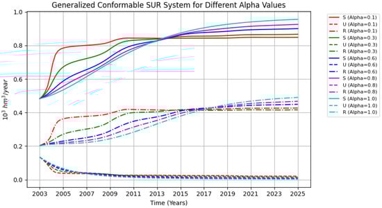
Figure 1.
Case 1 simulation for . It is important to note how, when using the conformable function , the transition zone at the beginning of the phenomenon becomes more pronounced.

Table 1.
Values obtained from the best fit for case 1.
Thus, the extended autonomous system from (10) is:
where both and are functions of t and . The dot represents the derivative with respect to time, and the given conditions are with respect to time. For brevity, the functional dependence on is omitted from the notation, but the reader should remember that these functions depend on .
To analyze the equilibrium points, we set the derivatives in (14) to zero, that is:
Next, we present several simulations conducted with different values of . We observe how different dynamics are obtained in each simulation.
Below are the values that were adjusted through least squares regressions, as shown in Section 3.1. For this, factors of and were used.
3.4. Homogeneous Case 2
We propose . To obtain the extended autonomous system with this choice of the conformable function, we find the differential equation that defines , which is given by . Thus, the extended autonomous system associated with (10) based on this choice of the conformable function is:
To perform the equilibrium point analysis, it suffices to set the derivatives to zero in (16), which yields:
Several graphs are presented below, generated by varying the parameter . The graphs appear to be similar, but there is a slight separation between them, particularly in the transition zones, where small phase shifts can be observed. In Table 2, the best fits are shown using regression models. The behaviors are clearly illustrated in Figure 2, highlighting how variations in affect the system’s dynamics.
Table 2.
Values obtained from the best fit for case 2.
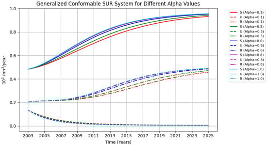
Figure 2.
Case 2: Graphs for , using the conformable function . The graph illustrates the slight phase shifts that occur as changes, especially in the transition zones.
3.5. Homogeneous Case 3
We propose . To derive the extended autonomous system with this choice of the conformable function, we find the differential equation that defines , given by . Therefore, the extended autonomous system associated with (10) with this choice of the conformable function is:
To analyze the equilibrium points, we set the derivatives to zero in (18), which yields:
Table 3 presents the fitting data for case 3. In contrast, the graphs can be observed in Figure 3. This example illustrates that for certain conformable functions, no significant changes are evident. This occurs because, when employing the least squares method to obtain the fitting values, the resulting graphs are virtually identical.
Table 3.
Values obtained from the best fit for case 3.
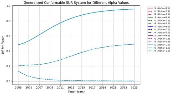
Figure 3.
Graphs for the conformable function with values = 0.1, 0.3, 0.6, 0.8, 1. It is important to note that the graphs overlap perfectly, indicating they are nearly identical.
3.6. Study of Equilibrium and Stability of the Model
In this section, we delve into the dynamics of the models, revealing that a coherent system consistently arises, regardless of the choice of . The following equations encapsulate this emerging framework:
Upon solving the system (20) using MATHEMATICA 12, the solutions obtained are:
For cases , and 3 with , the equilibrium points are found to be identical and take the following values:
We discard the points and since they have complex coordinates, rendering them physically meaningless for this study. Thus, we retain the points , and . Notably, the equilibrium states depend solely on the parameters , and .
We can analyze the stability of the system using a linear approximation around the equilibrium points. Let represent any equilibrium point of the system. Then, in the vicinity of this point, the system (13) with can be approximated as follows:
By analyzing the eigenvalues of the linearized system, we can gain insight into the dynamics of each equilibrium point. This is achieved by solving the determinant equation , where represents the Jacobian of the system evaluated at the equilibrium point E and is a conformable function. To facilitate the analysis of eigenvalues in a conformable dynamic system, we introduce the following lemma:
Lemma 3.
An autonomous dynamic system with homogeneous conformable derivatives exhibits the same behavior at its equilibrium points as the corresponding system with first-order derivatives.
Proof.
Consider the autonomous homogeneous conformable dynamic system:
where:
With as a conformable function. The system can be rewritten as follows:
where:
Let be an equilibrium point of the system. Then, we can perform a linear approximation in a neighborhood U containing as follows:
where is the Jacobian matrix of evaluated at the equilibrium point , which is a constant matrix.
As is well known, the type of stability of the system given by (24) depends on the sign of the eigenvalues of . Suppose we have the eigenvalues ; however, we need the eigenvalues of . These can be computed by solving for in the characteristic polynomial:
This implies:
This is the same polynomial but expressed as a function of , meaning it is , which will have roots . Since , the signs of the roots of and are the same, which is what we aimed to prove. □
Utilizing the result from Lemma 3 in the conformable SUR model, it suffices to analyze the eigenvalues of for to infer the dynamics at these equilibrium points. These eigenvalues are shown in Table 4.
Table 4.
Eigenvalues for the equilibrium points of .
Since and are attractors, this demonstrates that the amount of groundwater will inevitably decrease toward zero while the surface water and recharge stabilize at approximately and , respectively.
On the other hand, in case 1, the shape of the solution curve varies depending on the value of , leading to the following.
3.7. Combined Case
In this case, we will consider the homogeneous conformable linear combination function formed from the seven cases listed previously, specifically:
where:
To emphasize the role of the conformable functions in the model, we assigned the weight parameters , , and , with the specific aim of prioritizing the influence of , followed by , and finally . This weighting scheme was designed to ensure that the model captures the dominant dynamics associated with while still incorporating meaningful contributions from and . Based on this framework, the parameters are determined using a weighted average. If represents an aggregate parameter and for are the individual components, the combined parameter is calculated as follows:
For this study, is expressed as . It is crucial to acknowledge that the aforementioned weights were established through a process of proof and error, reflecting an intuitive approach to highlight the predominant contributions of each function. While this method provides a practical starting point, a detailed sensitivity analysis could offer a deeper understanding of the impact of the selected weight factors. However, such an analysis was not performed in this study as it falls beyond its current scope. Future research will aim to incorporate a comprehensive sensitivity analysis to evaluate the robustness and reliability of the model’s predictions under different weighting configurations. In Table 5, the information for the combined case is presented.
Table 5.
Combined data from the first three cases.
In Figure 4, we can observe the behavior of the dynamics of the combined case.
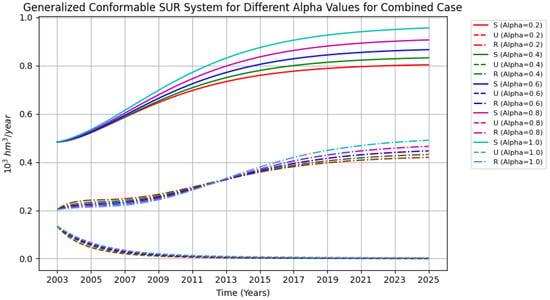
Figure 4.
Plot of the combined case. It is noteworthy that the curve exhibits an interesting spectrum. In contrast to cases 1, 2, and 3, the curves in this case show significant separation. The plot was generated for .
It is important to highlight that, unlike in cases 1, 2, and 3, the curves do not overlap in the combined case; instead, they progressively separate from each other. This separation allows for modeling a broader spectrum of behaviors, especially in the transition zone. While the overall behavior is similar to case 2, the increased weight applied to the function in the combined case results in a noticeable distinction between the curves. This shift in behavior can provide a more flexible approach for capturing a wider range of dynamics in systems with varying transition parameters.
4. Discussion
Our findings reveal that, due to the design of the model using generalized conformable calculus, the long-term behavior at equilibrium aligns with that of the classical integer-order model. However, depending on the choice of the conformable function, the aquifer dynamics in transitional zones can be better adapted to the specific conditions of the area. These conformable functions are selected heuristically, ensuring that the model more accurately reflects real-world behavior. The use of generalized conformable derivatives thus enhances the model’s capacity to capture and improve predictions specifically in these transitional zones.
A key advantage of this model is that it allows adjustments based on local data and information, enabling a tailored fit for each unique area of study. By employing regressions rather than strict fitting, the model mitigates the risk of overspecification, resulting in a more generalized and flexible representation of the system’s dynamics. This approach ensures that the model can be customized according to the characteristics of the study site, offering a robust tool for sustainable management in diverse regions.
Regarding the study area, the data were gathered from Pachuca de Soto, Hidalgo, a region located in central Mexico near the country’s capital. The model forecasts an overexploitation trend in the aquifer, indicating a depletion risk. This finding is consistent with predictions reported in [31], which also anticipates similar depletion behavior in the aquifer. Furthermore, our results align with the conclusions of [32], which affirmed that the aquifer is currently overexploited and moving toward a state of unsustainability.
Although this study successfully integrates generalized conformable derivatives to address the complexities of water resource management, certain limitations remain. Future research efforts will focus on refining the model’s predictive accuracy by integrating additional environmental variables and expanding the spatial scope of the study. Addressing these limitations in upcoming studies will help strengthen the model’s applicability and robustness, enhancing its utility for sustainable water management in semi-arid regions.
The modified Simplified Unified Resource (SUR) model offers several advantages, particularly in modeling non-stationary or transitional zones of hydrological phenomena. By employing generalized conformable derivatives, the model can adjust the order of differentiation (i.e., fractional order), providing a flexible tool that adapts to various system behaviors. This ability to tune the order of derivation ensures that the model can accommodate a wide range of data characteristics, improving accuracy in capturing the dynamics of the system. Additionally, it helps achieve better fitting for diverse datasets, making it a generalized model that can be tailored to any specific site with the necessary data. Once these data are gathered, the model can be adjusted quickly, reducing the complexity of its application.
Furthermore, the model’s long-term equilibrium behavior remains consistent, as confirmed by the Lemma 3, which states that the system’s equilibrium behavior is independent of the chosen conformable function or the order of differentiation. This means that, despite adjustments to these parameters, the equilibrium remains the same, ensuring that the model provides reliable predictions over time. Another significant advantage is the low number of parameters required, most of which can be obtained through data fitting or adjustment, making the model computationally efficient and easy to apply.
However, there are some limitations that need to be addressed. The current model does not account for factors such as pressure differences, porosity in infiltration processes, or other complex subsurface characteristics. Additionally, it lacks the ability to incorporate environmental variables directly, limiting its ability to represent interactions with external factors such as climatic variations or land use changes. It also does not currently support fuzzy logic or stochastic modeling, which are essential for capturing the inherent randomness and uncertainty in hydrological systems. As a mathematical model, it heavily relies on time-series data, and its accuracy depends on the quality and availability of these datasets, posing challenges in data-scarce regions.
Future research should aim to enhance the model by incorporating environmental variables directly into its framework, allowing for a more comprehensive representation of hydrological interactions. Furthermore, integrating stochastic or fuzzy logic components would improve the model’s robustness and capacity to handle uncertainty, further strengthening its predictive capabilities. These advancements would make the model more versatile and applicable to diverse, complex environmental conditions.
5. Conclusions
This study demonstrates that the SUR model significantly enhances the dynamics of groundwater systems. By applying conformable fractional derivatives, we captured the intricate behaviors of the model and established a framework that confirms the homotopy properties of the conformable linear combination function. Notably, we found that the phase space of the generalized conformable model aligns with that of the classical model, ensuring consistency in equilibrium states across both frameworks.
The introduction of the conformable derivative allows for a generalization of the system’s behavior, yielding a more versatile and complex dynamic. This adaptability is crucial for understanding the intricate interactions within the groundwater system. Furthermore, employing generalized sigmoid functions provides an effective means of modeling, showcasing the flexibility and robustness of our approach. Additionally, using conformable calculus improves modeling in the transition region. This analysis helps us better understand the behavior in this area because it is where there is more variation in the system. It is important to highlight that introducing this change in the original model aids in understanding regions where the derivative is far from zero, i.e., where the variation is greater. In contrast to [4], which used a sinusoidal function to obtain an oscillatory behavior, the dynamics in the transition zone are fixed. However, by using conformable calculus, we can adapt this dynamic behavior to simulate various outcomes.
Validation of our calculations was achieved using data from [4,33], specifically pertaining to the Pachuca de Soto, Hidalgo region. This validation underscores the reliability of our model and its applicability to real-world scenarios. Additionally, multiple linear regression was utilized to achieve optimal parameter fitting, reinforcing the accuracy of our results.
The simulations conducted across various cases illustrate how the choice of different conformable functions affects system dynamics. In Section 3.3, a pronounced transition zone is observed at the outset, accompanied by slight oscillations in the system. In Section 3.4, minor changes are noted in the transition zone, specifically a slight vertical phase shift of the functions. Conversely, as shown in Section 3.5, the selection of certain conformable functions can result in identical outcomes, indicating that significant variation is not always present.
Additionally, we introduced a combined Section 3.7, which demonstrates an averaged behavior derived from the other cases. This case can be used to simulate a dynamics formed by a linear combination of the others. A weighting factor was introduced to assign greater weight to one simulation over another, allowing us to control which dynamic is predominant. Since the conformable functions are presented heuristically, if several exhibit similar behaviors, they can be combined into one to improve the approximation.
An eigenvalue analysis conducted at the equilibrium points and confirmed their nature as attractors. This indicates that groundwater levels will inevitably decrease towards zero, while surface water and recharge levels stabilize around and , respectively.
It is important to highlight that the results yielded by the conformable model are consistent with those presented in [4] and validated by the data in that article.
This study presents findings with practical applications that can greatly benefit both local society and regional authorities. The insights from this model allow local decision-makers to better understand the dynamics and future trends of groundwater levels in Pachuca de Soto, Hidalgo, which is particularly valuable for regions facing similar semi-arid conditions. With an improved understanding of transition zones and equilibrium points, local authorities can make more informed decisions regarding water extraction and conservation practices. Furthermore, the flexibility of the model to be tailored to specific local conditions makes it a valuable tool not only for water resource planning in urban and rural settings in Hidalgo but also as a template for application in other semi-arid regions. By providing a model that can be adapted with data from different locations, this research has the potential to aid in the sustainable management of groundwater resources at a broader scale, offering insights for both local and national authorities in their efforts to ensure water availability for future generations.
In conclusion, this research offers valuable insights into groundwater dynamics by utilizing conformable fractional derivatives for modeling complex systems. As a different model that provides a distinct perspective through the way exchange rates and certain flow rates are modeled, this study takes reference from the previous work [4]. Future investigations should build upon these results by incorporating additional environmental factors and exploring the broader ecological implications, which may offer further advancements in understanding these dynamics.
Author Contributions
Conceptualization, J.N.G.-C. and G.F.-A.; methodology, J.N.G.-C. and G.F.-A.; software, J.N.G.-C.; validation, J.N.G.-C. and G.F.-A.; formal analysis, J.N.G.-C. and G.F.-A.; investigation, J.N.G.-C., G.F.-A., L.A.Q.-T. and A.T.-M.; resources, L.A.Q.-T. and A.T.-M.; data curation, J.N.G.-C., G.F.-A., L.A.Q.-T. and A.T.-M.; writing—original draft preparation, J.N.G.-C., G.F.-A., L.A.Q.-T. and A.T.-M.; writing—review and editing, J.N.G.-C., G.F.-A., L.A.Q.-T. and A.T.-M.; visualization, J.N.G.-C., G.F.-A., L.A.Q.-T. and A.T.-M. supervision, G.F.-A., L.A.Q.-T. and A.T.-M.; project administration J.N.G.-C., G.F.-A., L.A.Q.-T. and A.T.-M.; funding acquisition, L.A.Q.-T. and A.T.-M. All authors have read and agreed to the published version of the manuscript.
Funding
This research received no external funding.
Data Availability Statement
This study does not include any data availability information.
Acknowledgments
The first author would like to express his gratitude to CONAHCYT for the postgraduate scholarship and to Universidad Iberoamericana for the Excellence Scholarship. We would also like to thank DINVP for their support.
Conflicts of Interest
The authors confirm that they do not have any conflicts of interest that could affect the fairness or honesty of this study and/or the writing of this paper.
References
- Zewde, N.T.; Denboba, M.A.; Tadesse, S.A.; Getahun, Y.S. Predicting runoff and sediment yields using soil and water assessment tool (SWAT) model in the Jemma Subbasin of Upper Blue Nile, Central Ethiopia. Environ. Chall. 2024, 14, 100806. [Google Scholar] [CrossRef]
- Huang, Y.P.; Tsai, H.P.; Chiang, L.C. Integration of UAV Digital Surface Model and HEC-HMS Hydrological Model System in iRIC Hydrological Simulation—A Case Study of Wu River. Drones 2024, 8, 178. [Google Scholar] [CrossRef]
- El-Bagoury, H.; Gad, A. Integrated hydrological modeling for watershed analysis, flood prediction, and mitigation using meteorological and morphometric data, SCS-CN, HEC-HMS/RAS, and QGIS. Water 2024, 16, 356. [Google Scholar] [CrossRef]
- Gutiérrez-Corona, J.N.; Itzá-Ortiz, B.A.; Torres-Mendoza, A.; Tzatchkov, V.G.; Quezada-Téllez, L.A. Mathematical modeling for water supply by means of natural supply sources: The case of Pachuca de Soto, Hidalgo. Sustain. Water Resour. Manag. 2024, 10, 63. [Google Scholar] [CrossRef]
- Song, L. Dynamic Modeling and Simulation of Option Pricing Based on Fractional Diffusion Equations with Double Derivatives. Comput. Econ. 2024, 1–21. [Google Scholar] [CrossRef]
- López Gunn, E.; Rica, M.; Zugasti, I.; Hernaez, O.; Pulido-Velazquez, M.; Sanchis-Ibor, C. Use of the DELPHI method to assess the potential role of Enhanced Information Systems in Mediterranean groundwater management and governance. Water Policy 2024, wp2024033. [Google Scholar] [CrossRef]
- Lin, C.Y.; Alegria, M.E.O.; Dhakal, S.; Zipper, S.; Marston, L. PyCHAMP: A crop-hydrological-agent modeling platform for groundwater management. Environ. Model. Softw. 2024, 181, 106187. [Google Scholar] [CrossRef]
- Hassanzadeh, A.; Vázquez-Suñé, E.; Valdivielso, S.; Corbella, M. WaterpyBal: A comprehensive open-source python library for groundwater recharge assessment and water balance modeling. Environ. Model. Softw. 2024, 172, 105934. [Google Scholar] [CrossRef]
- Kenway, S.; Gregory, A.; McMahon, J. Urban water mass balance analysis. J. Ind. Ecol. 2011, 15, 693–706. [Google Scholar] [CrossRef]
- Gogo-Abite, I.; Chopra, M.; Wanielista, M. Integrated Surface–Groundwater Model for Storm-Water Harvesting Using Basic Mass Balance Principles. J. Irrig. Drain. Eng. 2013, 139, 55–65. [Google Scholar] [CrossRef]
- Bear, J.; Verruijt, A. Modeling Groundwater Flow and Pollution; Springer: Dordrecht, The Netherlands, 1987. [Google Scholar]
- Bear, J.; Cheng, A.H.D. Modeling Groundwater Flow and Contaminant Transport; Springer Science & Business Media: Berlin, Germany, 2010. [Google Scholar]
- Ntona, M.M.; Busico, G.; Mastrocicco, M.; Kazakis, N. Modeling groundwater and surface water interaction: An overview of current status and future challenges. Sci. Total Environ. 2022, 846, 157355. [Google Scholar] [CrossRef]
- Bhadula, R.C.; Pokhariyal, G.P.; Sisodia, M.; Mamgain, K.; Agarwal, I.; Bahuguna, A. Mathematical Model of Artificial Groundwater Recharge. Res. Sq. 2024. preprint. [Google Scholar] [CrossRef]
- Zhang, J.; Liang, X.; Zhang, Y.K.; Chen, X.; Ma, E.; Schilling, K. Groundwater responses to recharge and flood in riparian zones of layered aquifers: An analytical model. J. Hydrol. 2022, 614, 128547. [Google Scholar] [CrossRef]
- Celaya, S.; Fuente, I.; Rábago, D.; Quindós, L.; Sainz, C. Application of a mathematical model to an artificial aquifer under different recharge/discharge conditions using 222Rn as a tracer. Groundw. Sustain. Dev. 2022, 17, 100753. [Google Scholar] [CrossRef]
- Agnieszka, T. Numerical modeling and rational methods of water supply network operations in environmental engineering systems. Appl. Water Sci. 2023, 13, 18. [Google Scholar]
- Conejos Fuertes, P.; Martínez Alzamora, F.; Hervás Carot, M.; Alonso Campos, J. Building and exploiting a Digital Twin for the management of drinking water distribution networks. Urban Water J. 2020, 17, 704–713. [Google Scholar] [CrossRef]
- Keyhanpour, M.J.; Jahromi, S.H.M.; Ebrahimi, H. System dynamics model of sustainable water resources management using the Nexus Water-Food-Energy approach. Ain Shams Eng. J. 2021, 12, 1267–1281. [Google Scholar] [CrossRef]
- Haque, A.; Salama, A.; Lo, K.; Wu, P. Surface and groundwater interactions: A review of coupling strategies in detailed domain models. Hydrology 2021, 8, 35. [Google Scholar] [CrossRef]
- Nagata, K.; Shoji, I.; Arima, T.; Otsuka, T.; Kato, K.; Matsubayashi, M.; Omura, M. Practicality of integrated water resources management (IWRM) in different contexts. Int. J. Water Resour. Dev. 2022, 38, 897–919. [Google Scholar] [CrossRef]
- Diaz, M.; Sinicyn, G.; Grodzka-Łukaszewska, M. Modelling of groundwater–surface water interaction applying the hyporheic flux model. Water 2020, 12, 3303. [Google Scholar] [CrossRef]
- Nie, X.; Fan, T.; Wang, B.; Li, Z.; Shankar, A.; Manickam, A. Big data analytics and IoT in operation safety management in under water management. Comput. Commun. 2020, 154, 188–196. [Google Scholar] [CrossRef]
- INEGI. Climatología. 2024. Available online: https://www.inegi.org.mx/temas/climatologia/ (accessed on 11 November 2024).
- Khalil, R.; Al Horani, M.; Yousef, A.; Sababheh, M. A new definition of fractional derivative. J. Comput. Appl. Math. 2014, 264, 65–70. [Google Scholar] [CrossRef]
- Gateaux, R. Sur les fonctionnelles continues et les fonctionnelles analytiques. CR Acad. Sci. Paris 1913, 157, 65. [Google Scholar]
- Zhao, D.; Luo, M. General conformable fractional derivative and its physical interpretation. Calcolo 2017, 54, 903–917. [Google Scholar] [CrossRef]
- Smith, A.B.; Johnson, T.E.; Martinez, C.J. Understanding Surface Water Dynamics in Changing Environments. Water Resour. Res. 2021, 57, e2020WR028476. [Google Scholar] [CrossRef]
- Fleckenstein, J.H.; Krause, S.; Hannah, D.M. Groundwater–Surface Water Interactions: Recent Advances and Interdisciplinary Challenges. Water 2020, 12, 291. [Google Scholar]
- McDonald, J.A.; Newell, C.J.; Adamson, D.T.; Stroo, H.F. Modeling PFAS Fate and Transport in Groundwater, With and Without Precursor Transformation. Groundwater 2021, 59, 645–658. [Google Scholar]
- Ríos-Sánchez, K.I.; Chamizo-Checa, S.; Galindo-Castillo, E.; Acevedo-Sandoval, O.A.; González-Ramírez, C.A.; Hernández-Flores, M.d.l.L.; Otazo-Sánchez, E.M. The Groundwater Management in the Mexico Megacity Peri-Urban Interface. Sustainability 2024, 16, 4801. [Google Scholar] [CrossRef]
- Galindo, E.; Otazo, E.M.; Reyes, L.R.; Arellano, S.M.; Gordillo, A.; González, C.A. Balance hídrico y afectaciones a la recarga para el año 2021 en el acuífero Cuautitlán Pachuca. GeoFocus. Int. Rev. Geogr. Inf. Sci. Technol. 2010, 10, 65–90. [Google Scholar]
- Comisión Nacional del Agua. Sistema Nacional de Información del Agua (SINA). 2024. Available online: https://www.gob.mx/conagua/acciones-y-programas/sistema-nacional-de-informacion-del-agua-sina (accessed on 11 December 2024).
Disclaimer/Publisher’s Note: The statements, opinions and data contained in all publications are solely those of the individual author(s) and contributor(s) and not of MDPI and/or the editor(s). MDPI and/or the editor(s) disclaim responsibility for any injury to people or property resulting from any ideas, methods, instructions or products referred to in the content. |
© 2024 by the authors. Licensee MDPI, Basel, Switzerland. This article is an open access article distributed under the terms and conditions of the Creative Commons Attribution (CC BY) license (https://creativecommons.org/licenses/by/4.0/).