Global Water Use and Its Changing Patterns: Insights from OECD Countries

Abstract

Water resources are an important foundation for sustainable socioeconomic development. Revealing water use efficiency, the change in water use trends, and their driving mechanisms is essential for facilitating the scientific and reasonable prediction of water demand, thereby guiding the scientific planning and management of water resources. This study utilizes socioeconomic and water usage data from 65 countries spanning the years 1970 to 2020, employing the panel smooth transfer regression (PSTR) model to analyze the relationship between per capita total water withdrawal and per capita GDP. Additionally, Random Forest (RF) methods and empirical statistical analyses are implemented to identify the driving factors, control variables, and critical thresholds of water use trends in countries with different levels of development. The results show that: (1) there exists a nonlinear relationship between per capita total water withdrawal and per capita GDP on a global scale, with 70% of the countries exhibiting an inverted U-type trend in water usage; (2) the observed decline in per capita total water withdrawal in relation to per capita GDP is primarily driven by technological advancements and the optimization and enhancement of production structure; (3) common characteristics of OECD (Organization for Economic Cooperation and Development) countries that have reached their peak water usage include a service sector contribution to GDP exceeding 60%, urbanization levels at 70%, and per capita GDP surpassing USD 20,000. The observed changes in water use trends and the characteristic indicators associated with peak water usage, under conditions devoid of engineering interventions and resources constraints, can serve as valuable references for medium- and long-term water resources planning and water demand management in developing nations.

1. Introduction

A key issue for food production, ecological health, and socioeconomic development is the sustainable management of water resources [1,2]. Between 1900 and 2000, global water consumption surged more than eightfold, from 500 km³ per year to 4000 km³ per year [3]. Currently, approximately 3.6 billion people live in regions with limited water supplies, experiencing water shortages for at least one month each year. By 2050, it is projected that between 4.8 and 5.7 billion people will reside in water-scarce areas, primarily due to population growth in emerging nations [4,5]. Recent studies have highlighted the mismanagement of water resources, exacerbated by climate change, including the shrinkage of Aral Sea and the Dead Sea [6,7]; the Colorado River Basin, which has endured an extensive drought for over two decades [8]; the significant reduction in annual runoff of Yellow River, which reached its lower level in 2016 and 2017 [9]; and the ongoing depletion of groundwater supplies in heavily irrigated regions, such as the Ogallala Aquifer in the western United States [10]. The United Nation’s World Population Prospects 2024: Summary of Results report anticipates that the global population will peak at 10.3 billion in the mid-2080s, underscoring water scarcity as a major global concern.

In addition to inadequate natural resources, poor management is often directly linked to water scarcity [11,12]. Graham et al. [13] emphasized that the success of any water resource development project critically depends on the accuracy and reliability of forecasts for future water demand during its planning and management phases. Previous medium- and long-term predictions for water resources needs have consistently overestimated actual consumption levels [14]. For example, in the mid-1990s, actual global water consumption was only approximately half of what had been projected three decades earlier. Since 1990, the potential for water resources development under the “Business-As-Usual” (BAU) scenario has been significantly underestimated worldwide, with substantial deviations being observed between departments and countries compared with the existing trends in water use. Currently, per capita domestic water consumption has surpassed the projections for the year 2025 under the BAU scenario [15]. Many predictions of the Organization for Economic Cooperation and Development (OECD) about water demands in the 1960s and 1970s were overly ambitious. Most countries’ forecasted growth rates were significantly higher than those actually achieved. Two forms of detailed evidence support this: the results are substantially lower than the original forecasts, and the long-term predictions have been drastically reduced [16]. The situation in China is similarly illustrative; for example, a report in 1986 predicted that total water demand in 2000 would be 709.6 billion m³, while the National Medium- and Long-term Water Supply and Demand Plan report in 1998 predicted a total water demand 600 billion m³ for the same year. In reality, total water consumption in China was 549.8 billion m³ in 2000, the figure falling far below the prediction values [17].

There are several reasons why the forecasted values significantly deviate from actual water usage. On one hand, limitations in water supply conditions, such as inadequate water supply engineering capacity, result in insufficient supply and restrictions on overall water management. On the other hand, deficiencies exist in the methods used to predict water demand. Commonly employed methods, such as the quota method [18], trend analysis method [19], and statistical method [20], heavily rely on historical data and statistical relationships while insufficiently considering the driving mechanisms and principles that govern water resources supply and demand. These mechanisms include institutions factors, economic development trends, and contributions of technological progress. This oversight can lead to prediction failures. Therefore, scientifically sound and well-reasoned water development plans can mitigate the waste or scarcity caused by either over-exploitation or under-exploitation of water resources. The precision and utility of global water development strategies can be significantly enhanced by considering the response relationships between water use and economic growth, historical water use trends, and the impact mechanisms of the key driving factors. Our objective is to address three primary research issues: (1) Is there a significant trend relationship between water use and economic growth? (2) What are the spatial and temporal patterns of global water use? (3) What factors drive changes in water use trends? To investigate these questions, we employ the panel smooth transition regression (PSTR) model, along with various statistical analyses, to examine the relationship between water use and economic structure, regional geography, GDP, and other relevant variables. Additionally, we utilize Random Forest (RF) methods and empirical statistical analyses to identify the driving factors, control factors, and critical thresholds for different water resources.

In the intricate socioeconomic activities related to water resources, various factors—including levels of economic and social development, fluctuations in water resources availability, patterns of water usage, agricultural structures and scales, water supply conditions, and technological advancement often exhibit nonlinear relationships. To effectively capture these nonlinear characteristics within a modelling framework, regional conversion models are frequently utilized due to comprehensively explain phenomena while maintaining simplicity and ease of operation. Based on different assumptions regarding district–system conversion behaviors, these models can be categorized into three primary types: smooth conversion, retarded models, and Malthusian district system conversion. The essence of the PSTR model lies in its ability to allow regression coefficients to transition gradually from one group to another. This gradual change ensures that functions containing external variables are continuous and smooth across different extreme regional systems. This feature aligns well with the characteristics of the changes observed in water resources. González et al. [21] were pioneers in applying the PSTR model. By extending the framework of the panel threshold regression (PTR) model introduced by Hansen [22], they relaxed its constraints and incorporated a smooth transition via a logistic function. This innovation effectively addresses the abrupt changes observed in the threshold regression models, thereby overcoming the mutation phenomenon.

The driving mechanism serves as a pivotal force that can influence the state or performance of a system. It provides insights into past and present occurrences within an entire system, including its internal dynamics, and establishes a foundation for predicting future trends. Since the mid-20th century, human impact on the Earth’s systems has dramatically intensified, which is often referred to as the “Great Acceleration”. Steffen et al. [23] emphasized that forecasts of water demand are highly sensitive to assumptions regarding socioeconomic drivers such as economic growth. For example, Wada et al. [2,24,25] and Wada and Bierkens [26] utilized socioeconomic, technological, and agricultural driving factors to estimate the water demand, withdrawal, and consumption of various sectors on a 0.5° global grid from 1960 to 2099. Soligno et al. [3] identified six key socioeconomic driving factors—economic structural changes, GDP, population density, and agriculture—to quantify the main socioeconomic factors influencing global blue water use trends through the MRIO framework from 1994 to 2010. Their findings suggest that increasing wealth is the primary determinant of the rising global water use trend. Similarly, Gupta et al. [27] and Sun et al. [28] reported that economic growth and population expansion have significantly increased the global water demand. The enhancement of water use efficiency is regarded as the primary catalyst for mitigating the human impact on water resources [29]. The United Nations report on Sustainable Development Goals 6.4.2 (SDGs 6.4.2) reported that water scarcity has increased globally in most countries, whereas water scarcity has decreased in 44 countries [30]. However, the leading factors contributing to global water scarcity or reduction remain unclear; therefore, identifying the main driving factors influencing water availability is crucial for the sustainable management of global water resources.

The contribution of this study lies in the application of mathematical models and empirical case analyses to examine the evolving trends and key driving factors affecting global water resources. Our research findings provide valuable insights for the sustainable utilization and management of global water resources. This paper is structured as follows: Section 2 introduces the research data and analysis methods; Section 3 summarizes the research findings; Section 4 discusses the driving factors, control variables, and critical thresholds associated with changes in water usage; and Section 5 presents the conclusions drawn from the research.

2. Data and Methods

2.1. Data

The annual data on the water withdrawal, GDP, and socioeconomic indicators in different countries are from the Global Information System on Water and Agriculture (AQUASTAT) of the Food and Agriculture Organization of the United Nations (FAO) (see

Table 1. Variables and units of AQUASTAT datasets.

Variables	Units	Variables	Units
Agricultural water withdrawal	m3	Industry, value added to GDP	USD
Agriculture, value added to GDP	USD	Municipal water withdrawal	m3
Cultivated area (arable land + permanent crops)	ha	Services, value added to GDP	USD
GDP deflator (2015)		Total renewable water resources per capita	m3/inhab
GDP	USD	Total population	inhab
Industrial water withdrawal	m3	Urban population	inhab

). AQUASTAT’s extensive database is primarily populated by information sourced from national statistical agencies, with a keen focus on monitoring and managing water resources, overall water withdrawal, and agricultural water use across countries worldwide. This withdrawal dataset is meticulously assembled through advanced modelling techniques, interpolation of relevant reports, and continuous updates to the original measurement data, all aimed at ensuring the highest level of quality and precision. AQUASTAT contains data on water withdrawals from different industries and water sources in various countries around the world, as well as socioeconomic indicators related to water resources, and the data time series are long and comprehensive. The results will be more comparative and more scientific and reasonable. Despite the existence of certain data gaps, AQUASTAT stands as one of the most exhaustive and frequently referenced repositories for global water statistics [31,32,33].

Temperature and precipitation data, which are the primary climate factors influencing changes in water usage, were obtained from the National Centers for Environmental Information (NCEI) of the National Oceanic and Atmospheric Administration (NOAA). The NCEI provides one of the most extensive environmental data archives in the world, encompassing surface meteorological observation data from more than 35,000 stations globally. These data are updated with remarkable frequency—every hour, every three hours, and daily.

2.2. Research Methods

Figure 1 illustrates a flowchart for analyzing the changing modes of global water usage and the driving factors behind them.

To achieve this, we first use the PSTR model and mathematical statistical methods to correctly understand the relationship between per capita total water abstinence and per capita GDP, thereby presenting the overall level of global water (Section 3.1). Next, we utilize mathematical statistical methods to analyze the trends in total water withdrawals and per capita water withdrawal, correlating these metrics with changes in per capita GDP (Section 3.2) and presenting the spatial patterns of global water use (Section 3.3). Finally, based on six key dimensions, we use an RF model and the experience statistics method to identify the driving factors of different water use modes, control factors, and key thresholds (Section 4.1 and Section 4.2).

2.2.1. Panel Smooth Transition Regression Model

The PSTR model is used in this study to analyze the changing characteristics of global water use, based on data concerning per capita total water withdrawal and per capita GDP across 65 countries, covering the period from 1970 to 2020. The explanatory variable of the PSTR model is set as per capita total water withdrawal, and the explanatory variable and conversion variable are set as per capita GDP. These variables play crucial roles in mitigating data fluctuations, eliminating temporal sequence discrepancies, reducing extreme values, and addressing abnormal distributions, thereby ensuring robust and reliable analysis across different regions.

“Water withdrawal” refers to the storage or use of water transported from its source to different locations; some of this water may return to the original source with changes in both volume and quality, whereas some is consumed. The term “consumptive use” describes the use of water in a variety of ways, including transpiration, soil absorption, product adsorption, and livestock drinking. “Consumption use” is critical indicator for measuring changes in water shortages and can effectively reflect the scarcity of water resources and the environmental impact assessments [34]. Unfortunately, data on consumption are often not easy to obtain. However, there is a strong correlation between “water withdrawal” and “consumptive use”, and “consumptive use” can be a reasonable substitute for “water withdrawal”. Total water withdrawals are predominantly influenced by population growth trends, and the extent of the impact of other factors may not be adequately analyzed. However, the per capita total water withdrawal indicator can compensate for the limitations of aggregate water use metrics, making them suitable as dependent variables. GDP serves as an indicator of economic growth, with per capita GDP mitigating the influence of varying population sizes. Additionally, to eliminate the effects of price fluctuations, the GDP deflator is used to convert per capita GDP based on the year 2015 as the base period. All analyses involving GDP indicators throughout the text are conducted using this adjusted per capita GDP. The basic form of the PSTR model is shown in Equation (1):

$$Y_{\mathrm{it}}={\mu }_i+{\beta }_0^{\prime }{X}_{\mathrm{it}}+{\beta }_1^{\prime }{X}_{\mathrm{it}}\mathrm{g}\left({\mathrm{q}}_{\mathrm{it}};\gamma ,c\right)+{\epsilon }_{\mathrm{it}}$$

(1)

where, i = 1.N and t = 1.T, where N and T represent the number of cross-sections and the temporal dimension of the panel data, respectively; let Y_it be the logarithm of the dependent variable for country i in year t, let X_it be the logarithm of the independent variable for country i in year t, let μ_i be the fixed effect for country i, let ε_it be the standard error term, let β₀ be the regression coefficient for the linear part of the independent variable, let β₁ be the regression coefficient for the nonlinear part of the independent variable, and let g(q_it; γ; c) be the transformation function, with a value range between [0, 1]. The formula is shown in Equation (2):

$$\mathrm{g}\left(q_{it};\gamma ,c\right)={\left(1+\exp \left(-\gamma \left({\displaystyle \prod _{j=1}^m\left(q_{it}-c_j\right)}\right)\right)\right)}^{-1}, \gamma >0$$

(2)

In the equation, q_it represents the threshold variable; c_j denotes the location parameter; γ is the smoothness parameter, also known as the slope of the transition function; and m signifies the number of location parameters in the transition function.

Wald tests, Fisher tests, or LRT tests are employed to conduct cross-sectional heteroscedasticity tests (linearity tests) and non-retention heteroscedasticity tests (nonlinearity tests) on the PSTR model. The formula is shown in Equation (3):

$$LM={\displaystyle \frac{TN\left(SS{R}_0-SS{R}_1\right)}{SS{R}_0}} LMF={\displaystyle \frac{\left(SS{R}_0-SS{R}_1\right)/\mathrm{m}K}{SS{R}_0/\left(TN-N-\mathrm{m}K\right)}} LRT=-2\log {\displaystyle \frac{SS{R}_1}{SS{R}_0}}$$

(3)

In the equation, K represents the number of explanatory variables; SSR₀ denotes the sum of the squared residuals under the null hypothesis; and SSR₁ represents the sum of the squared residuals under the alternative hypothesis. The LMF statistic follows a $F\left(mK,TN-N-mK\right)$ distribution under the null hypothesis, whereas the LM and LRT statistics both follow a ${\chi }^2\left(mK\right)$ distribution.

The optimal number of location parameters m is determined according to the application of the Akaike information criterion (AIC) and the Bayesian information criterion (BIC).

2.2.2. Drivers of Water Use

The variable importance measure (VIM) is utilized to assess the significance of sample features and to quantitatively describe their contributions to classification or regression tasks [35]. The RF is extensively employed for classification, regression, and dimensionality reduction. This method exhibits resilience against noise, superior generalization capabilities, and a reduced tendency towards overfitting [36,37]. The mean decrease accuracy (MDA) index, which is based on the out-of-bag (OOB) data permutation, and the mean decrease impurity (MDI) index, which is based on the Gini index, are the two primary categories of RF-based feature significance evaluation metrics. The MDA index, which is popular, avoids the bias problem with the MDI index by directly measuring the degree to which each feature variable affects the accuracy of the model. The fundamental concept of the MDA index based on OOB data permutation can be stated as follows. Only the order of a particular feature variable in the OOB data is modified, disrupting the correlation between the feature variable and the output in the OOB data while maintaining the other feature variables as unaltered. The original and scrambled OOB data are then predicted via decision trees. The significance of that feature variable is determined by averaging the mean squared errors of all the decision trees before and after shuffling [37].

The RF method was used in this study to assess the significance of the individual characteristic variables in influencing changes in per capita total water withdrawal. The evaluation spans 15 indicators, encompassing six key dimensions: development scale, water use structure, production structure, production level, water resources condition, and climate change. This comprehensive analysis was conducted for 65 countries worldwide with a series length of 1970–2020.

Table 2. Possible explanatory variables and their descriptions of water use.

Indicator Category	Acronym	Description	Unit
Development scale	CA	Cultivated area (arable land + permanent crops)	ha
	GDP	Gross domestic product	USD
	Urb	Urbanization	%
Water Resources condition	Trwrpc	Total renewable water resources per capita	m3/inhab
Production structure	Agr-GDPA	Agriculture, value added (% GDP)	%
	Ind-GDPA	Industrial, value added (% GDP)	%
	Ser-GDPA	Services, value added (% GDP)	%
Water use structure	Agr-TWW	Agricultural water withdrawals as % of total water withdrawals	%
	Ind-TWW	Industrial water withdrawals as % of total water withdrawals	%
	Mun-TWW	Municipal water withdrawals as % of total water withdrawals	%
Production level	AgrUSE	Agricultural water use efficiency	USD/m3
	IndUSE	Industrial water use efficiency	USD/m3
	SerUSE	Services water use efficiency	USD/m3
Climate change	Pre	Precipitation	mm
	Tem	Temperature	°C

presents the potential explanatory variables related to water use alongside their respective descriptions, offering insight into the multifaceted factors driving variations in per capita total water withdrawal. Development scale serves as a pivotal driver of water consumption dynamics. Economic expansion is gauged by GDP and varies considerably across nations due to the differences in resources availability, population, and development policies implemented. The speed of development mainly determines the growth rate of water use. Urbanization (Urb) changes water use mainly by driving secondary and tertiary industries to become the main body of the national economy, and the agricultural labor force gradually shifts to non-agricultural industries. Urb can drive water use up through improvements in living standards and changes in lifestyle and can also reduce water use through the advancement of water-saving technology. The cultivated area (CA), which is the largest sector of global water use, directly affects changes in agricultural water use. The water resources condition significantly influences regional patterns of water use for both production and domestic purposes to a certain extent and shapes residents’ consciousness of water conservation. Certain aspects of water resources availability act as catalysts, fueling demand for water resources, fostering economic development, and enhancing quality of life. Conversely, other conditions serve to mitigate water demand and increase water use efficiency. This complex interplay is encapsulated by the variable Trwrpc, which quantifies the ratio between a nation’s renewable water resources and its population size, thereby providing insight into the relative abundance or scarcity of per capita water resources. The adjustment of production structure and water use structure can effectively modulate changes in water use, and the impact of these adjustments is reflected primarily in the proportional relationships between the output values and water consumption across the municipal, industrial, and agricultural sectors. Production level can effectively reduce water consumption, which is represented by the ratio of total water use to the added value per USD 10,000 in an industry. Climate elements have been in a process of constant fluctuation and oscillation for a long time, and the climate change dimension has direct or indirect impacts on water use, which are represented by precipitation (Pre) and temperature (Tem).

3. Results

3.1. Overall Level of Global Water Use

Before estimating the parameters of the PSTR model, it is necessary to conduct linear and nonlinear residual tests via Wald tests, Fisher tests, or LRT tests.

Table 3. Results of the linear and nonlinear residual tests.

	m = 1			m = 2
	LM	LMF	LRT	LM	LMF	LRT
Linear tests (H0: r = 0; H1: r = 1)	20.913 (0.000)	20.540 (0.000)	20.999 (0.000)	20.957 (0.000)	10.288 (0.000)	21.043 (0.000)
2 transition functions (H0: r = 2; H1: r = 3)	2.728 (0.099)	2.657 (0.103)	2.729 (0.099)	8.250 (0.016)	4.025 (0.018)	8.264 (0.016)
AIC	11.766			11.769
BIC	11.779			11.786

Note: The values in parentheses are the corresponding p values.

shows that for both m = 1 and m = 2, the global LM, LMF, and LRT statistics all reject the null hypothesis (H₀: r = 0) of a linear relationship at the 1% significance level, indicating the presence of a nonlinear effect between global per capita total water withdrawal and per capita GDP. In both scenarios where m = 1 and m = 2, the initial assumption H₀: r = 2 cannot be rejected. The global PSTR model incorporates two nonlinear transition functions. The AIC and BIC are employed to ascertain the optimal value of m. For the parameter m = 1, the calculated AIC is 11.766 and the BIC is 11.779, both of which are lower than those for m = 2, where the AIC stands at 11.769 and the BIC at 11.786. This indicates a preference for the simpler model with one positional parameter. The econometric analysis of the PSTR model reveals the nuanced impact of global per capita GDP on per capita total water withdrawal across distinct intervals.

Compared with the results in 1995, total global water withdrawals globally (from 65 countries) in 2020 increased by 10.85%, while per capita total water withdrawal decreased by 19.31%. Figure 2 illustrates the trend of per capita total water withdrawal in relation to per capita GDP, featuring both curve fitting (dashed line) and linear fitting (solid line) for global data (a) and OECD countries (b). The relationships between per capita total water withdrawal and per capita GDP exhibit an inverted U-type in both 1995 and 2020. Notably, the fitting curve for OECD countries in 1995 provides compelling evidence: in low-income countries, per capita total water withdrawal increases as per capita income rises. Conversely, in middle-income countries, per capita total water withdrawal shows no significant correlation with changes in income levels [38]. In high-income countries, per capita total water withdrawal decreases significantly as income increase.

3.2. Trends in Global Water Use

A case analysis was conducted on the trends in total water withdrawals and per capita total water withdrawal from 1970 to 2020 across 65 countries. These metrics were correlated with changes in per capita GDP. The analysis identified three distinct water use trends: inverted U-type (a), rising type (b), and wave type (c), as illustrated in Figure 3. The inverted U-type is exemplified by the United States of America (USA), which shows that per capita total water withdrawal or total water withdrawals initially increase with per capita GDP growth, reach a peak, and then decrease as the economy further develops. The rising type is demonstrated by Algeria, which indicates a continuous increase in per capita total water withdrawal, or total water withdrawals as per capita GDP increases. The wave type is represented by Denmark, revealing that per capita total water withdrawal or total water withdrawals fluctuate as per capita GDP increases.

The trends in per capita total water withdrawal with respect to per capita GDP are inverted U-type, rising-type, and wave-type relationships, accounting for 66%, 11%, and 23%, respectively, of the countries in the world. Among the OECD countries, the inverted U-type countries include the USA, Japan, Spain, and 21 others; the wave-type countries include Australia, Denmark, the United Kingdom, and 8 others; and the rising-type countries consist of Türkiye and Colombia. For the non-OECD group of 27 countries, the inverted U-type countries include China, Egypt, Brazil, and 16 more; the wave-type countries include Tunisia, India, and Kazakhstan; and the rising-type countries include Algeria, Argentina, Cuba, Indonesia, and South Africa. Approximately three-fourths of the countries in the world have the same water use trends for total water withdrawals and per capita total water withdrawal, and one-fourth of the countries with different water withdrawal trends have basically increased their total water withdrawals (except Japan and Morocco). Among these countries, China, Egypt, Eswatini, India, Iran, Pakistan, United Republic of Tanzania, Uruguay, and Viet Nam are showing a plateauing trend in their total water withdrawals, indicating that economic development and technological advancements offset the growth in water use driven by the scale of development activities in developing countries.

3.3. Spatial Patterns of Global Water Use

It can be observed from Figure 4 that, from a spatial distribution perspective, countries where per capita total water withdrawal and total water withdrawals following the inverted U-type and wave-type trends with changes in per capita GDP are located mainly in Europe, Americas, Oceania, and North Asia. This may be related to improved water use efficiency caused by higher economic levels and industrial upgrades offsetting the increase in water use due to population growth and rising living standards. Countries of the rising type are found mainly in Africa, parts of Asia, and Latin America. Among them, Israel, China, and most other countries primarily experience an increase in total water withdrawals due to rapid population growth and improved living standards. Similarly, Alcamo et al. [39] and Soligno et al. [3] reached similar conclusions. For example, between 1970 and 2020, Israel’s population density tripled, municipal water withdrawals quadrupled, and total water withdrawals increased by nearly 50%, Kramer et al. [40] also have a similar opinion. In New Zealand and Iceland, the main reason for the increase in total water withdrawals is agricultural water withdrawals, whereas in Ghana and the United Republic of Tanzania, it is the combined effect of population growth, improved living standards, and an increased proportion of agricultural water withdrawals that leads to continuous increases in total water withdrawals.

4. Discussion

4.1. Drivers of Water Use Trends

A comprehensive analysis was conducted on 43 countries, encompassing both 24 OECD countries and 19 non-OECD countries, to examine the declining trend in per capita total water withdrawal correlated with fluctuations in per capita GDP from 1970 through 2020. This rigorous assessment involved evaluating 15 distinct characteristic variables across six pivotal dimensions: development scale, water use structure, production structure, production level, water resources condition, and climate change. Each variable was meticulously assessed for its unique contribution to understanding the dynamics behind the observed shifts in per capita total water withdrawal over this extensive timeframe. The analysis depicted in Figure 5a clearly reveals that socioeconomic development stands as the primary driving force behind the decrease in per capita total global water withdrawal. The influence of climate change, while present, appears to be minimal, aligning with the findings of numerous scholars [39,41,42,43,44,45]; specifically, TRWRPC, Urb, SerUSE, IndUSE, and GDP are the main factors affecting the decrease in per capita total water withdrawal. Notably, the enhancement of services and industry production levels plays a pivotal role in mitigating the per capita total water withdrawal decrease observed in OECD countries; conversely, the reduced share of water utilized in agriculture significantly contributes to the decrease in per capita total water withdrawal in non-OECD countries, as illustrated in Figure 5b. The decrease in Agr-TWW is an important factor influencing the decrease in the amount of per capita total water withdrawn in non-OECD countries. The primary factors affecting agricultural water withdrawals include irrigation water use efficiency, production scale, pre, and planting structure. For example, the main reason for the decrease in agricultural water withdrawals in Afghanistan is the significant compression of irrigation areas caused by the contradiction between water supply and demand, and the main reason for the decrease in agricultural water withdrawals in Mexico is the improvement in irrigation water use efficiency.

Simultaneously, nations such as Switzerland, Libya, Venezuela, Canada, Romania, and Iran have exhibited a prolonged phase of stability in their per capita total water withdrawal, closely mirroring the trends in per capita GDP. Specifically, from 1975 to 1990, Venezuela experienced a plateau from 1970 to 2000; Canada’s stable period extended from 1982–2014; Romania maintained a consistent level between 1981 and 1993; and Iran saw a steady withdrawal rate from 1995 to 2003. The underlying factor contributing to this extended stability in per capita water withdrawal for countries such as Iran and Switzerland remains under investigation. In inverted U-type countries, the average annual proportions of municipal, industrial, and agricultural water withdrawals were 21%, 34%, and 45%, respectively, whereas in wave-type countries, the average annual proportions of municipal, industrial, and agricultural water withdrawals were 29%, 27%, and 45%, respectively. In countries where per capita total water withdrawal shows inverted U-type or wave-type trends with per capita GDP, the Mun-TWW reached 45%, whereas the Agr-TWW was relatively low.

From 1970 to 2020, seven countries, namely, Algeria, Argentina, Cuba, Indonesia, South Africa, Türkiye and Colombia, had increased per capita total water withdrawal with per capita GDP. In addition to the above seven countries, there are 14 other countries where total water withdrawals have increased with per capita GDP, including China, Egypt, and India. Except for Türkiye and Colombia, all other countries are non-OECD countries. The primary factors influencing per capita total water withdrawal and total water withdrawals include affluence and population growth. Additionally, the Agr-TWW in countries where per capita total water withdrawal increased from 1970 to 2020 averaged at 70%, and agriculture has always been the most important water-using sector.

4.2. Control Factors and Critical Thresholds

Compared with the substantial economic costs associated with direct water reduction measures, enhancing production efficiency or implementing structural upgrades is a more effective strategy. In 2020, global water withdrawals by agriculture, industry, and municipal sectors accounted for 48%, 28%, and 23% of the total, respectively, highlighting agriculture as the world’s predominant water-consuming sector. Notably, the distribution varies significantly across continents: in North America, 51% of its water withdrawals come from agriculture, South America is at 48%, and Europe is at a comparatively lower 15%. Agriculture accounts for more than 75% of water withdrawals in Africa and Asia, 64% in Oceania, 51% in North America, 48% in South America, and 15% in Europe. In contrast, Ind-TWW in Europe (50%), North America (30%), and South America (36%) are relatively high. Regional differences in municipal water withdrawals range from 13% to 34% in Europe and 34% in other regions. The European and American continents, which have relatively high industrial water intakes, contribute significantly to the per capita total global water withdrawal. These regions exhibit inverted U-type or wave-type changes in per capita GDP, closely aligning with the rising-type trends. Furthermore, nations experiencing an inverted U-type GDP trajectory have experienced a substantial decrease in Agr-GDPA, whereas Ser-GDPA has experienced rapid growth. In scenarios where the economic scale remains constant, industries with high water use play a crucial role in mitigating the reduction in total water resources.

Another primary catalyst behind the global stability or decrease in water use is the advancement of water-saving technologies, particularly the enhancement of production efficiency within the industrial and service sectors. For example, water use trends in USA increased significantly from 1950 to 1980, stabilized from 1950 to 1980, and then decreased sharply from 1950 to 1980, decreasing by 118.15 billion m³, illustrating a classic inverted U-type trend. From 1990 to 2020, the average annual of Ind-TWW was 51.77%, making it the largest consumer of water in the country. From 2005 to 2015, there was a significant reduction in industrial water withdrawals of approximately 95.4 billion m³; it can be attributed primarily to reduce coal use and the adoption of more efficient power generation and cooling system technologies [46,47]. Water use highlights improvements in efficiency as a key driver in reducing industrial water withdrawals. In four countries—Luxembourg, New Zealand, South Korea, and Switzerland—where the trend of change is predominantly driven by municipal water withdrawals, the primary reason for the declining water use is the substantial growth in the services and industry production levels; this growth has effectively offset the increased water demand caused by continuous population growth and rising Urb levels.

In this study, we examined data on per capita total water withdrawal in relation to per capita GDP at its peak for 22 OECD countries and Singapore (non-OECD), as illustrated in Figure 6a. Our analysis reveals that the peak values for most of these countries occurred between 1980 and 2000. This period coincided with the largest increase in Ser-GDPA, which is basically above 60%; Agr-GDPA typically accounted for less than 10%. Additionally, during this time, the Urb exceeded 50%, with over two-thirds of the countries surpassing an Urb of 70%. In most countries, the per capita GDP exceeds USD 10,000, with more than two-thirds surpassing USD 20,000. Figure 6b illustrates the per capita peak water use in relation to per capita GDP for 13 non-OECD countries. The analysis indicates that the majority of these countries reached their peak water use after 1990, primarily because of agricultural water withdrawals, which account for more than 60% of the total use. Notably, more than two-thirds of these countries have agricultural water withdrawals that exceed 85%.

5. Conclusions

This study, which utilized data from 65 countries over the period from 1970 to 2020, employed the PSTR model to elucidate the relationship between per capita total water withdrawal and per capita GDP, Furthermore, Random Forest and empirical statistical analyses were conducted to reveal the driving factors, control factors, and critical thresholds associated with various trends in water usages. The key findings are as follows:

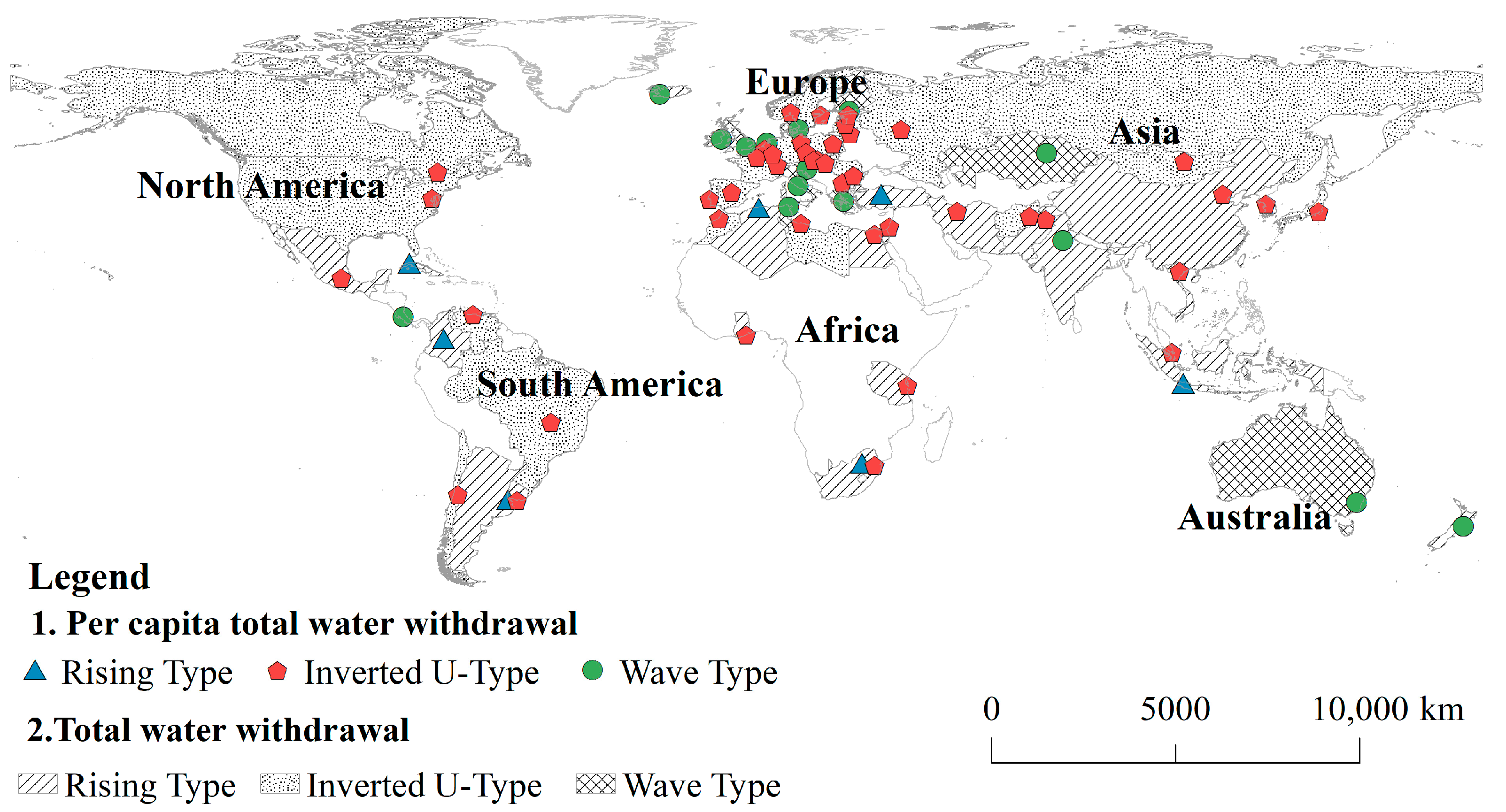
(1)

At the global level, trends in water use can be categorized into three primary types: rising type, inverted U-type, and wave type. Notably, countries exhibiting an inverted U-type trend in per capita total water withdrawal represent approximately 70% of the global total. From a spatial distribution perspective, the inverted U-type and wave-type trends are predominantly observed in Europe, the Americas, Oceania, and North Asia. In contrast, the rising type is primarily evident in Africa, certain regions of Asia, and Latin America.

(2)

The per capita total water withdrawal is significantly influenced by improvements in water use efficiency, particularly evident in the plateaus and declines observed within OECD countries. Conversely, structural upgrades play a crucial role in the reduction of water consumption in non-OECD countries. Technological innovations and structural upgrades are vital for decreasing municipal and industrial water withdrawals while ensuring stability in agricultural water withdrawals. However, these strategies alone are insufficient to address the persistent challenges posed by severe constraints on water resources. Additional factors, such as the urbanization, the level of economic development, and policy guidance, also significantly impacts trends in water consumption.

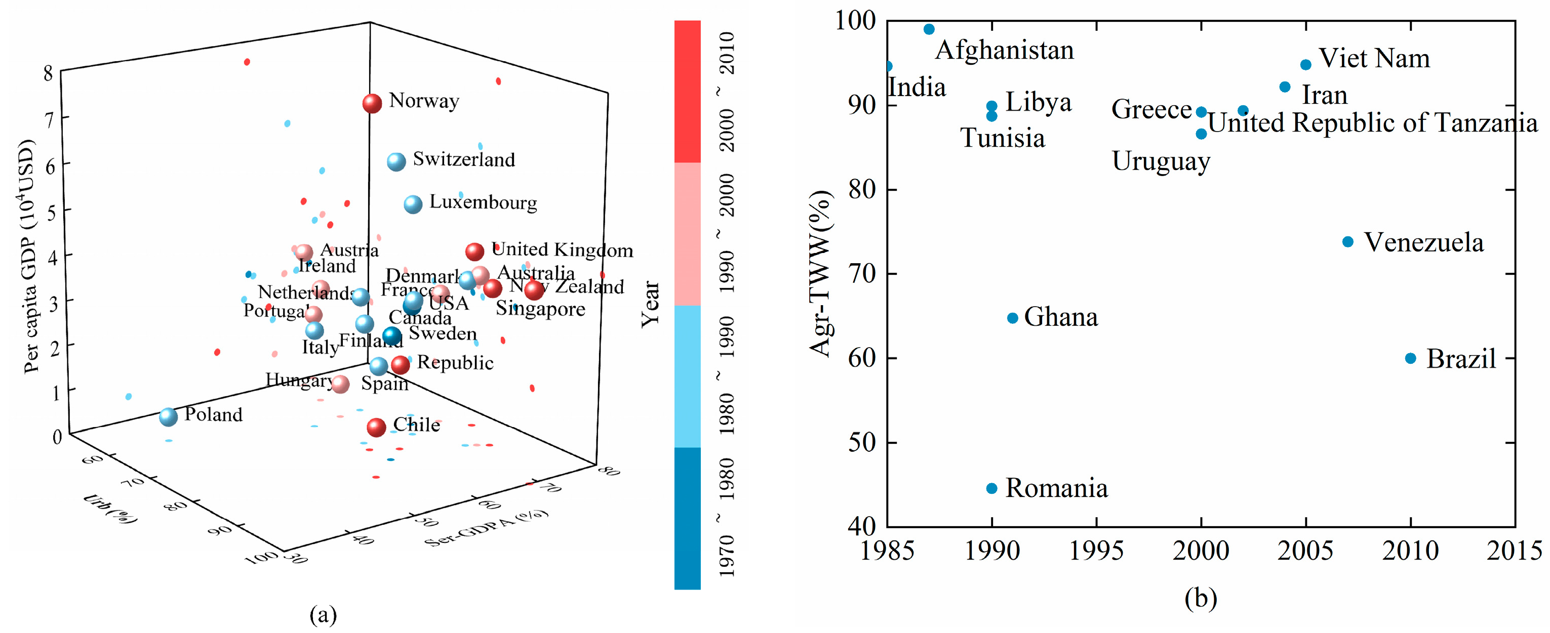
(3)

When water usage in OECD countries reaches its peak, the Ser-GDPA generally exceeds 60%, the urbanization rate surpasses 70%, and the per capita GDP exceeds USD 20,000. Analyzing the development trend of agricultural water withdrawals will be crucial for non-OECD countries to accurately project future water demand.

This study provides evidence that enhances the precision of forecasts related to water resources demand and offers significant insights into how nations are adapting to manage drought conditions. Future research should be conducted utilizing more reliable data and indicators, with a focus on comprehensive analyses of water usage patterns and factors across various sectors, including municipal, industrial, and agricultural, as well as diverse water sources, both conventional and non-conventional. Additionally, it is crucial to investigate how these research findings can be applied to the demand for water resources. Given to the complexities associated with climate change and human activities, an analysis of global water resource utilization and evolving patterns can help water resource managers and policy-makers in reformulating strategies for water resources planning and management, thereby mitigating unnecessary economic costs of expanding water infrastructure and minimizing adverse environmental impacts.

References

- Zubaidi, S.L.; Al-Bugharbee, H.; Ortega-Martorell, S.; Gharghan, S.K.; Olier, I.; Hashim, K.S.; Al-Bdairi, N.S.; Kot, P. A novel methodology for prediction urban water demand by wavelet denoising and adaptive neuro-fuzzy inference system approach. Water 2020, 12, 1628. [Google Scholar] [CrossRef]
- Wada, Y.; van Beek, L.P.; Bierkens, M.F. Modelling global water stress of the recent past: On the relative importance of trends in water demand and climate variability. Hydrol. Earth Syst. Sci. 2011, 15, 3785–3808. [Google Scholar] [CrossRef]
- Soligno, I.; Malik, A.; Lenzen, M. Socioeconomic drivers of global blue water use. Water Resour. Res. 2019, 55, 5650–5664. [Google Scholar] [CrossRef]
- WWAP (United Nations World Water Assessment Programme). The United Nations World Water Development Report 2018: Nature-Based Solutions. Paris. UNESCO. Available online: www.unwater.org/publications/world-water-development-report-2018/ (accessed on 8 October 2024).
- Munia, H.A.; Guillaume, J.H.; Wada, Y.; Veldkamp, T.; Virkki, V.; Kummu, M. Future transboundary water stress and its drivers under climate change: A global study. Earth’s Future 2020, 8, e2019EF001321. [Google Scholar] [CrossRef] [PubMed]
- Su, Y.; Li, X.; Feng, M.; Nian, Y.; Huang, L.; Xie, T.; Zhang, K.; Chen, F.; Huang, W.; Chen, J.; et al. High agricultural water consumption led to the continued shrinkage of the Aral Sea during 1992–2015. Sci. Total Environ. 2021, 777, 145993. [Google Scholar] [CrossRef]
- AI-Mashagbah, A.F.; Ibrahim, M.; Al-Fugara, A. Estimation of changes in the Dead Sea surface water area through multiple water index algorithms and geospatial techniques. Glob. Nest J. 2021, 23, 565–571. [Google Scholar] [CrossRef]
- Hung, F.; Son, K.; Yang, Y.E. Investigating uncertainties in human adaptation and their impacts on water scarcity in the Colorado river Basin, United States. J. Hydrol. 2022, 612, 128015. [Google Scholar] [CrossRef]
- Chen, Y.P.; Fu, B.J.; Zhao, Y.; Wang, K.B.; Zhao, M.M.; Ma, J.F.; Wu, J.H.; Xu, C.; Liu, W.G.; Wang, H. Sustainable development in the Yellow River Basin: Issues and strategies. J. Clean. Prod. 2020, 263, 121223. [Google Scholar] [CrossRef]
- Cruse, R.M.; Devlin, D.L.; Parker, D.; Waskom, R.M. Irrigation aquifer depletion: The nexus linchpin. J. Environ. Stud. Sci. 2016, 6, 149–160. [Google Scholar] [CrossRef]
- Mehta, L. Water and Human Development. World Dev. 2014, 59, 59–69. [Google Scholar] [CrossRef]
- Leijnse, M.; Bierkens, M.F.; Gommans, K.H.; Lin, D.; Tait, A.; Wanders, N. Key drivers and pressures of global water scarcity hotspots. Environ. Res. Lett. 2024, 19, 054035. [Google Scholar] [CrossRef]
- Graham, N.T.; Hejazi, M.I.; Chen, M.; Davies, E.G.; Edmonds, J.A.; Kim, S.H.; Turner, S.W.; Li, X.; Vernon, C.R.; Calvin, K.; et al. Humans drive future water scarcity changes across all Shared Socioeconomic Pathways. Environ. Res. Lett. 2020, 15, 014007. [Google Scholar] [CrossRef]
- Shiklomanov, I.A. Appraisal and assessment of world water resources. Water Int. 2000, 25, 11–32. [Google Scholar] [CrossRef]
- Cosgrove, W.J.; Rijsberman, F.R. Water Futures. In World Water Vision: Making Water Everybody’s Business; Cosgrove, W.J., Rijsberman, F.R., Eds.; Routledge: London, UK, 2000; pp. 23–48. [Google Scholar] [CrossRef]
- Herrington, P. Water Demand Forecasting in OECD Countries; Environment Directorate, Organisation for Economic Co-Operation and Development: Paris, France, 1987. [Google Scholar]
- Zhao, Y.; Li, H.; Liu, H.; Wang, L.; He, G.; Wang, H. The law of growth: Prediction of peak water consumption in China. J. Hydraul. Eng. 2021, 52, 129–141. [Google Scholar] [CrossRef]
- Daniell, K.A.; Rinaudo, J.D.; Chan, N.W.W.; Nauges, C.; Grafton, Q. Long-Term Water Demand Forecasting. In Understanding and Managing Urban Water in Transition; Rinaudo, J.D., Ed.; Global Issues in Water Policy; Springer: Dordrecht, The Netherlands, 2015; Volume 15, pp. 239–419. [Google Scholar] [CrossRef]
- Donkor, E.A.; Mazzuchi, T.A.; Soyer, R.; Alan Roberson, J. Urban water demand forecasting: Review of methods and models. J. Water Resour. Plan. Manag. 2014, 140, 146–159. [Google Scholar] [CrossRef]
- Guo, L.; Zhu, W.; Wei, J.; Wang, L. Water demand forecasting and countermeasures across the Yellow River basin: Analysis from the perspective of water resources carrying capacity. J. Hydrol. Reg. Stud. 2022, 42, 101148. [Google Scholar] [CrossRef]
- González, A.; Teräsvirta, T.; van Dijk, D. Panel Smooth Transition Regression Models; Quantitative Finance Research Centre, University of Technology: Sydney, Australia, 2005. [Google Scholar]
- Hansen, B.E. Sample splitting and threshold estimation. Econometrica 2000, 68, 575–603. [Google Scholar] [CrossRef]
- Steffen, W.; Broadgate, W.; Deutsch, L.; Gaffney, O.; Ludwig, C. The trajectory of the Anthropocene: The great acceleration. Anthr. Rev. 2015, 2, 81–98. [Google Scholar] [CrossRef]
- Wada, Y.; Wisser, D.; Eisner, S.; Flörke, M.; Gerten, D.; Haddeland, I.; Hanasaki, N.; Masaki, Y.; Portmann, F.T.; Stacke, T.; et al. Multimodel projections and uncertainties of irrigation water demand under climate change. Geophys. Res. Lett. 2013, 40, 4626–4632. [Google Scholar] [CrossRef]
- Wada, Y.; Wisser, D.; Bierkens, M.F. Global modeling of withdrawal, allocation and consumptive use of surface water and groundwater resources. Earth Syst. Dyn. 2014, 5, 15–40. [Google Scholar] [CrossRef]
- Wada, Y.; Bierkens, M.F. Sustainability of global water use: Past reconstruction and future projections. Environ. Res. Lett. 2014, 9, 104003. [Google Scholar] [CrossRef]
- Gupta, R.; Yan, K.; Singh, T.; Mo, D. Domestic and international drivers of the demand for water resources in the context of water scarcity: A cross-country study. J. Risk Financ. Manag. 2020, 13, 255. [Google Scholar] [CrossRef]
- Sun, S.; Zheng, X.; Liu, X.; Wang, Z.; Liang, L. Global pattern and drivers of water scarcity research: A combined bibliometric and geographic detector study. Environ. Monit. Assess. 2022, 194, 523. [Google Scholar] [CrossRef] [PubMed]
- Zhou, F.; Bo, Y.; Ciais, P.; Dumas, P.; Tang, Q.; Wang, X.; Liu, J.; Zheng, C.; Polcher, J.; Yin, Z.; et al. Deceleration of China’s human water use and its key drivers. Proc. Natl. Acad. Sci. USA 2020, 117, 7702–7711. [Google Scholar] [CrossRef] [PubMed]
- Water, U.N. Progress on Level of Water Stress: Global Baseline for SDG Indicator 6.4. 2. UN Water, 24 August 2018. Available online: https://www.unwater.org/publications/progress-on-level-of-water-stress-642/ (accessed on 10 August 2024).
- Gleick, P.H.; Cooley, H. Freshwater scarcity. Annu. Rev. Environ. Resour. 2021, 46, 319–348. [Google Scholar] [CrossRef]
- Katz, D. Water use and economic growth: Reconsidering the Environmental Kuznets Curve relationship. J. Clean. Prod. 2015, 88, 205–213. [Google Scholar] [CrossRef]
- Song, Z.; Jia, S. Municipal water use Kuznets curve. Water Resour. Manag. 2023, 37, 235–249. [Google Scholar] [CrossRef]
- Cole, M.A. Economic growth and water use. Appl. Econ. Lett. 2004, 11, 1–4. [Google Scholar] [CrossRef]
- Chen, R.C.; Dewi, C.; Huang, S.W.; Caraka, R.E. Selecting critical features for data classification based on machine learning methods. J. Big Data 2020, 7, 52. [Google Scholar] [CrossRef]
- Gaines, M.D.; Tulbure, M.G.; Perin, V. Effects of climate and anthropogenic drivers on surface water area in the southeastern United States. Water Resour. Res. 2022, 58, e2021WR031484. [Google Scholar] [CrossRef]
- Song, S.; He, R.; Shi, Z.; Zhang, W. Variable importance measure system based on advanced random forest. Comput. Model. Eng. Sci. 2021, 128, 65–85. [Google Scholar] [CrossRef]
- Amarasinghe, U.A.; Smakhtin, V. Global Water Demand Projections: Past, Present and Future; International Water Management Institute (IWMI): Colombo, Sri Lanka, 2014; Volume 156, p. 32. [Google Scholar] [CrossRef]
- Alcamo, J.; Flörke, M.; Märker, M. Future long-term changes in global water resources driven by socio-economic and climatic changes. Hydrol. Sci. J. 2007, 52, 247–275. [Google Scholar] [CrossRef]
- Kramer, I.; Tsairi, Y.; Roth, M.B.; Tal, A.; Mau, Y. Effects of population growth on Israel’s demand for desalinated water. Npj Clean Water 2022, 5, 67. [Google Scholar] [CrossRef]
- Shen, Y.; Oki, T.; Kanae, S.; Hanasaki, N.; Utsumi, N.; Kiguchi, M. Projection of future world water resources under SRES scenarios: An integrated assessment. Hydrol. Sci. J. 2014, 59, 1775–1793. [Google Scholar] [CrossRef]
- Veldkamp, T.I.; Wada, Y.; de Moel, H.; Kummu, M.; Eisner, S.; Aerts, J.C.; Ward, P.J. Changing mechanism of global water scarcity events: Impacts of socioeconomic changes and inter-annual hydro-climatic variability. Glob. Environ. Chang. 2015, 32, 18–29. [Google Scholar] [CrossRef]
- Fant, C.; Schlosser, C.A.; Gao, X.; Strzepek, K.; Reilly, J. Projections of water stress based on an ensemble of socioeconomic growth and climate change scenarios: A case study in Asia. PLoS ONE 2016, 11, e0150633. [Google Scholar] [CrossRef] [PubMed]
- Wada, Y.; Flörke, M.; Hanasaki, N.; Eisner, S.; Fischer, G.; Tramberend, S.; Satoh, Y.; Van Vliet, M.T.H.; Yillia, P.; Ringler, C.J.G.M.D.; et al. Modeling global water use for the 21st century: The Water Futures and Solutions (WFaS) initiative and its approaches. Geosci. Model Dev. 2016, 9, 175–222. [Google Scholar] [CrossRef]
- Distefano, T.; Kelly, S. Are we in deep water? Water scarcity and its limits to economic growth. Ecol. Econ. 2017, 142, 130–147. [Google Scholar] [CrossRef]
- Donnelly, K.; Cooley, H. Water Use Trends in the United States; Pacific Institute: Oakland, CA, USA, 2015; Available online: https://pacinst.org/publication/water-use-trends-in-the-united-states (accessed on 8 September 2024).
- Konar, M.; Marston, L. The water footprint of the United States. Water 2020, 12, 3286. [Google Scholar] [CrossRef]