Monthly Runoff Prediction Based on Stochastic Weighted Averaging-Improved Stacking Ensemble Model

Abstract

The accuracy of monthly runoff predictions is crucial for decision-making and efficiency in various areas, such as water resources management, flood control and disaster mitigation, hydraulic engineering scheduling, and agricultural irrigation. Therefore, in order to further improve the accuracy of monthly runoff prediction, aiming at the problem that the traditional Stacking ensemble method ignores (the base model correlation between different folds in the prediction process), this paper proposes a novel Stacking multi-scale ensemble learning model (SWA–FWWS) based on random weight averaging and a K-fold cross-validation weighted ensemble. Then, it is evaluated and compared with base models and other multi-model ensemble models in the runoff prediction of two upstream and downstream reservoirs in a certain river. The results show that the proposed model exhibits excellent performance and adaptability in monthly runoff prediction, with an average RMSE reduction of 6.44% compared to traditional Stacking models. This provides a new research direction for the application of ensemble models in reservoir monthly runoff prediction.

1. Introduction

Monthly runoff prediction serves as a fundamental basis for water resource planning and management. Its accuracy directly affects the operational efficiency and safety of various fields, such as hydropower generation [1,2,3], ecological protection [4,5], meteorological detection [6], and flood control [7,8,9,10]. Therefore, improving runoff prediction models by incorporating regional monthly runoff characteristics is crucial for enhancing prediction accuracy. This, in turn, plays a significant role in formulating scientific water resource management strategies, optimizing water allocation, mitigating natural disaster risks, and promoting sustainable development [11].

Currently, runoff prediction models commonly used in the field of runoff prediction are mainly divided into two categories: process-driven models and data-driven models. Process-driven models, such as the Xinanjiang Model [12] and Numerical Weather Prediction (NWP) [13,14], are capable of simulating watershed hydrological cycles based on physical mechanisms, offering strong physical interpretability. However, due to the complexity of natural hydrological processes and the large amount of data required, constructing data-driven models becomes more challenging [15,16].

In recent years, with the development of artificial intelligence and deep learning technologies, data-driven models, which focus on learning to map relationships between data sets, have gradually replaced process-driven models based on physical mechanisms and taken a dominant position. Data-driven models predict unknown data by learning the mapping relationship between input factors and runoff, which has the significant advantages of easy model construction, wide range of application, and high prediction accuracy. In runoff prediction, common data-driven models include the support vector machine (SVM) [17,18,19,20], random forest (RF) [21,22,23,24,25], autoregressive moving average (ARMA) [26,27], and long-short-term memory network (LSTM) [28,29,30,31,32]. Samantaray et al. [33] combined SVM with the Sparrow Search Algorithm (SSA), proposing an SVM-SSA model for monthly runoff prediction under different climate characteristics. Chen et al. [34] introduced the LSTM-ALSL model, which takes into account both short and long lag times, improving rainfall-runoff prediction accuracy. Li et al. [35] transformed traditional time series runoff prediction into a supervised learning problem using LSTM. Their results demonstrated that this approach mitigates overfitting issues in deep learning models while enhancing the prediction accuracy of LSTM. Although the common data-driven model has the advantages of high computational efficiency, in the face of complex and high-latitude runoff data, a single data-driven model with a simple structure sometimes cannot fully capture the nonlinear correlation within the data, making it unable to effectively complete the complex runoff prediction task.

To overcome the limitations of a single data-driven model, researchers have proposed multiple ensembled models for runoff prediction by combining multiple models based on methods such as the Weighted Average ensemble [36,37,38], Blending [39], AdaBoost [40] and Stacking [41,42,43]. These ensemble models improve the overall predictive performance of the model by fusing different underlying models. However, traditional multi-model weighted ensemble methods have certain limitations in the allocation of model weights [44,45]. To address this, Yao et al. [46] applied an adaptive weighting method to ensemble CNN-LSTM and GRU-ISSA models, using an improved Sparrow Search Algorithm for hyperparameter optimization. The proposed model was found to demonstrate superior predictive performance and remarkable adaptability. In addition, in order to try to use the AdaBoost ensemble technique for rainfall-runoff models, Liu et al. [47] used the improved AdaBoost.RT algorithm as an ensemble method for the hydrological model XXT, so as to propose the AdaBoost-XXT ensemble model and use it for process-based rainfall-runoff models. The results show that the model not only improves the prediction accuracy of the rainfall-runoff model but also demonstrates a better generalization ability. Lu et al. [48] integrated the attention mechanism with the Stacking ensemble model to improve the accuracy and stability of daily runoff prediction. All of the above studies integrated or improved models on a multi-model scale and did not combine single-model ensemble methods with multi-model ensemble methods. Furthermore, the conventional stacking model fails to consider the inter-model correlation when confronted with an identical training set during cross-validation in the ensemble process. This ultimately constrains the prediction performance of the mining base model across different folds to a certain degree.

Therefore, to address the above problems, this study first proposes an improved Stacking ensemble method, Fold-Wise Weighted Stacking (FWWS), which takes the model obtained by integrating the Stochastic Weight Averaging (SWA) of the single-model ensemble method and the deep learning model as the basic model. The base models are then integrated using a fold-wise weighted ensemble approach through K-fold cross-validation, and the proposed FWWS multi-model ensemble method is used as an ensemble. This approach establishes connections between the base models across different folds, resulting in the multi-scale SWA–FWWS model for monthly runoff prediction. The study reveals that the coupled base models not only enhance prediction accuracy but also improve the generalization ability of the ensemble model; the SWA–FWWS model also achieves better monthly runoff prediction results. The main innovations of this study are as follows:

This study proposes an improved Stacking ensemble method and uses it to integrate deep learning models such as LSTM, GRU, and TCN to construct an FWWS model for monthly runoff prediction, thereby improving prediction accuracy.

The study innovatively couples the single-model ensemble method of stochastic weight averaging with the proposed multi-model ensemble method (FWWS) to construct the SWA–FWWS model, which further enhances the prediction accuracy and generalization ability of monthly runoff prediction models.

Finally, this study evaluates and compares the monthly runoff prediction performance of the SWA–FWWS model with other ensemble models on different reservoirs in a certain river. The prediction performance and generalization ability of the proposed model are demonstrated.

The chapters of this paper are arranged as follows: Section 1 introduces the research background of this paper. Section 2 introduces the basic model used in this paper, the proposed improved SWA–FWWS model, and the evaluation criteria of model. Section 3 introduces the runoff data from two hydropower stations, A and B, in the river, and describes the study area and data, the data preprocessing, and the design of simulation and comparison experiments in this paper. Section 4 presents the experimental results of the proposed model and the comparison model with a total of ten groups of models. Section 5 and Section 6 present the discussion and conclusions of this paper, respectively.

2. Methodology

2.1. Deep Learning Models

2.1.1. Long Short-Term Memory (LSTM)

Long Short-Term Memory (LSTM) is a special type of Recurrent Neural Network (RNN) primarily used for processing and predicting long-term dependencies in time series data. It was proposed by Hochreiter and Schmidhuber in 1997 [49].

A typical LSTM unit consists of the following parts:

Forget gate $f_t$: Determines how much of the previous time step’s state is forgotten.

$$f_t=\sigma (W_f\cdot [h_{t-1},x_t]+b_f)$$

(1)

Input gate $i_t$: Determines how much of the current state is updated.

$$i_t=\sigma \left(W_i\cdot \left[h_{t-1},x_t\right]+b_i\right)$$

(2)

$${\tilde{C}}_t=tanh(W_C\cdot [h_{t-1},x_t]+b_C)$$

(3)

Update of the memory cell $C_t$: Combines the forget gate and input gate to update the state.

$$C_t=f_t \ast C_{t-1}+i_t \ast {\tilde{C}}_t$$

(4)

Output gate $O_t$: Determines how much of the current state is output.

$$O_t=\sigma \left(W_o\cdot \left[h_{t-1},x_t\right]+b_o\right)$$

(5)

$$h_t=O_t \ast tanh\left(C_t\right)$$

(6)

where $t$ is the time step, $h$ represents the time output, $x$ is the input, $\sigma$ is the sigmoid activation function, $tanh$ is the hyperbolic tangent function, $W$ and $b$ are the weight matrix and bias vector, respectively, and ${\tilde{C}}_t$ is the candidate memory cell.

2.1.2. Gated Recurrent Unit (GRU)

The Gated Recurrent Unit (GRU) is an effective variant of the LSTM network. Unlike LSTM, the GRU model features only two gates: the update gate $Z_t$ and the reset gate $R_t$ [50]. The update gate regulates how much of the prior state is carried forward into the current state. The reset gate determines the amount of past state information that influences the current candidate set $H_{t-1}$. The GRU formulae are as follows:

Reset gate:

$$R_t=\sigma (X_t{W}_{xr}+H_{t-1}{W}_{hr}+b_r)$$

(7)

Update gate:

$$Z_t=\sigma (X_t{W}_{xz}+H_{t-1}{W}_{hz}+b_z)$$

(8)

Candidate state:

$${\tilde{H}}_t=\mathrm{t}\mathrm{a}\mathrm{n}\mathrm{h}(X_t{W}_{xh}+\left(\begin{array}{c}{R}_t\odot H_{t-1}\end{array}\right)W_{hh}+b_h)$$

(9)

Current state:

$$H_t=Z_t\odot H_{t-1}+(1-Z_t)\odot {\tilde{H}}_t$$

(10)

Output:

$$Y_t=H_t{W}_{hq}+b_q$$

(11)

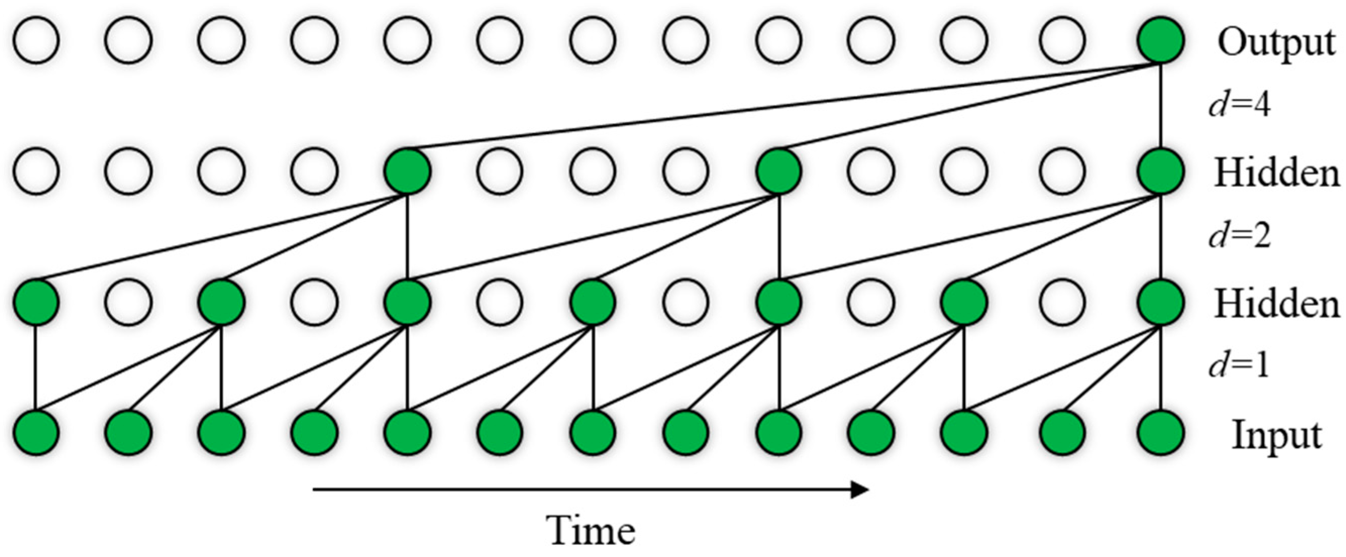
2.1.3. Temporal Convolutional Network (TCN)

The Temporal Convolutional Network (TCN) is a neural network introduced by Bai et al. [51], which incorporates causal convolution, dilated convolution, and a residual block. Compared to traditional recurrent neural networks or convolutional networks, the TCN can better process and predict time series data [52]. Unlike traditional convolutional structures, the TCN allows the input to be sampled at intervals during the convolution process. As the layers increase, the effective window size grows exponentially, enabling the model to capture local features over different time scales. Therefore, even with fewer layers, the TCN can achieve a large receptive field, capturing intricate patterns in the data [53].

Assuming the input sequence is $x$ and the model is set with a series of convolution kernels $f:\left\{\begin{array}{c}0,\dots ,k-1\end{array}\right\}$, the output of the t-th neuron after dilated convolution is given by:

$$F\left(t\right)=\sum _{i=0}^{k-1}f\left(i\right)·x_{t-d·i}$$

(12)

where $k$ is the convolution kernel size, $d$ is the dilation factor, $f\left(i\right)$ represents the i-th element of the convolution filter, and $x_{t-d·i}$ represents the input value at time t shifted by $d·i$ steps into the past.

Figure 1 illustrates the structure of a dilated causal convolution stack with filter size $k=3$ and dilation factor $d=[1,2,4]$.

In addition, in order to improve the stability of the network when constructing the deep network and to prevent the problem of gradient disappearance and model degradation in model training, the TCN adopts the idea of a residual network to construct the residual connection network, which includes the dilated causal convolution layer, the weight normalization layer, the activation function ReLU, and the dropout layer, as shown in Figure 2.

In view of the superiority and stability of LSTM, GRU, and TCN in dealing with the long-term dependencies of time series data, these three models were adopted as the basic models in this study.

2.1.4. Light Gradient Boosting Machine (LightGBM)

The Light Gradient Boosting Machine (LightGBM) algorithm is a learning algorithm based on a gradient boosting decision tree proposed in 2017 [54]. Its core principle is to train the model by iteratively constructing decision trees and correcting the residuals of the previous decision trees, so as to gradually optimize the prediction performance of the model and realize various prediction tasks. Compared with the XGBoost algorithm, LightGBM further enhances the computational efficiency and generalization ability of the model by introducing a histogram-based algorithm, Leaf-wise tree growth strategy, Exclusive Feature Bundling (EFB), and a Gradient-based One-Side Sampling (GOSS) algorithm on its foundation.

In view of the advantages of high computational efficiency and strong generalization ability in the face of high-dimensional features, we chose LightGBM as the meta model of the ensemble model in this study.

2.2. Stochastic Weighted Average (SWA)

Stochastic Weight Averaging (SWA) [55] is an efficient ensemble technique based on the weight space of a single model, which can significantly enhance the generalization ability of deep learning models to improve prediction accuracy. Research has shown that during the training process of deep learning models, due to the influence of learning rates and uncontrollable factors, the loss value tends to converge toward the edge of a set of good weight spaces, fluctuating as the model weights are updated [56]. The optimal solution located at the center of this weight space generally has better generalization capability. Therefore, by employing a cyclical learning rate schedule (such as a cosine annealing learning rate or linear decay learning rate) toward the end of the model training process and capturing model parameters at fixed intervals (i.e., edge solutions near the center of the weight space) $W_1$, $W_2$, $W_3$, the average of these parameters yields a better solution at the center of the weight space, denoted as $W_{SWA}$.

In this study, we adopted the more stable cosine annealing learning rate as the SWA method for adjusting the learning rate of the base model. The principle of a cosine annealing learning rate is illustrated in Figure 3, where the learning rate fluctuates between the maximum value ${\alpha }_{max}$ and the minimum value ${\alpha }_{min}$ following a cosine curve for each cycle. After several cycles, the model parameters corresponding to the minimum learning rate at the end of each cycle are averaged to obtain the final model parameters.

2.3. The Proposed SWA–FWWS Model for Monthly Runoff Prediction

This section innovatively proposes a Fold-Wise Weighted Stacking multi-model ensemble method based on stochastic weight averaging of the cosine annealing learning rate and the K-fold cross-validation weighted ensemble, then uses it to construct the proposed SWA–FWWS monthly runoff prediction model. The SWA-ensembled base models were obtained by applying the SWA single-model ensemble method with a cosine annealing learning rate to multiple deep learning models. Then, the K-fold cross-validation and the proposed FWWS multi-model ensemble method were used to carry out a multi-model ensemble operation based on fold-wise weighting on the obtained basic model, so as to establish the linkage of the base models among different folds and obtain the multi-scale ensemble model SWA–FWWS of monthly runoff prediction to improve the overfitting phenomenon of multi-model ensembles in monthly runoff prediction. The construction of the SWA–FWWS model mainly includes the following steps:

(1)

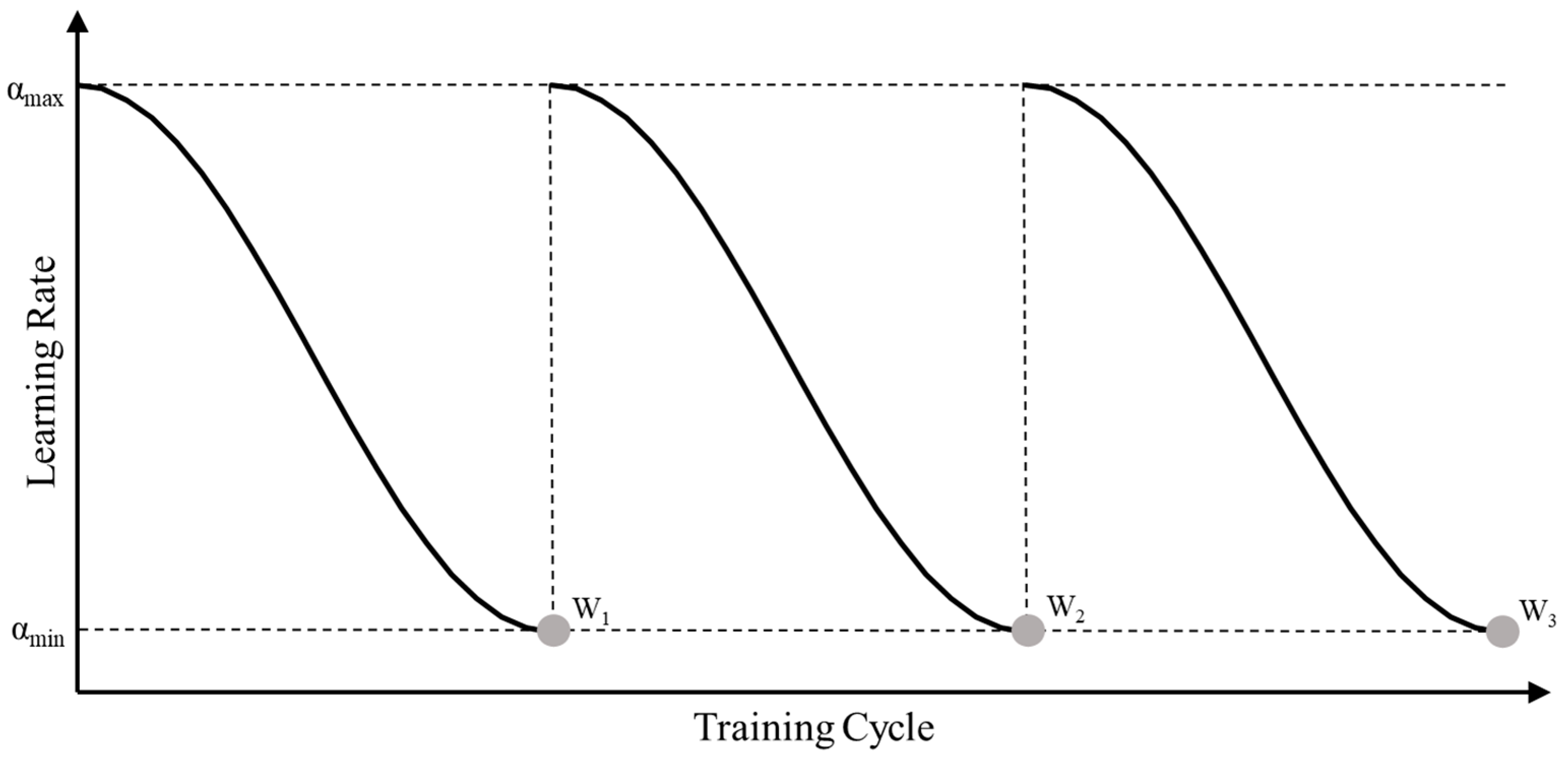
Set hyper-parameters for the SWA. This includes determining the upper and lower bounds of the learning rate ${\alpha }_{max}$ and ${\alpha }_{min}$ when using the SWA algorithm, the total training cycles $T$, the starting cycle for ensembling $T_s$, the learning rate adjustment period $t$, and the number of cycles $s$. The hyper-parameters should satisfy $T=t \ast s+T_s$.

(2)

Perform single-model ensembles for multiple deep learning models using SWA. Each deep learning model begins training with the maximum learning rate ${\alpha }_{max}$. When the training cycle reaches $T_s$, the learning rate is adjusted to the cosine annealing schedule. During each model’s training process, the model parameters are recorded and averaged each time the learning rate reduces to ${\alpha }_{min}$. These averaged parameters are used as the final parameters for an SWA-ensembled base model.

(3)

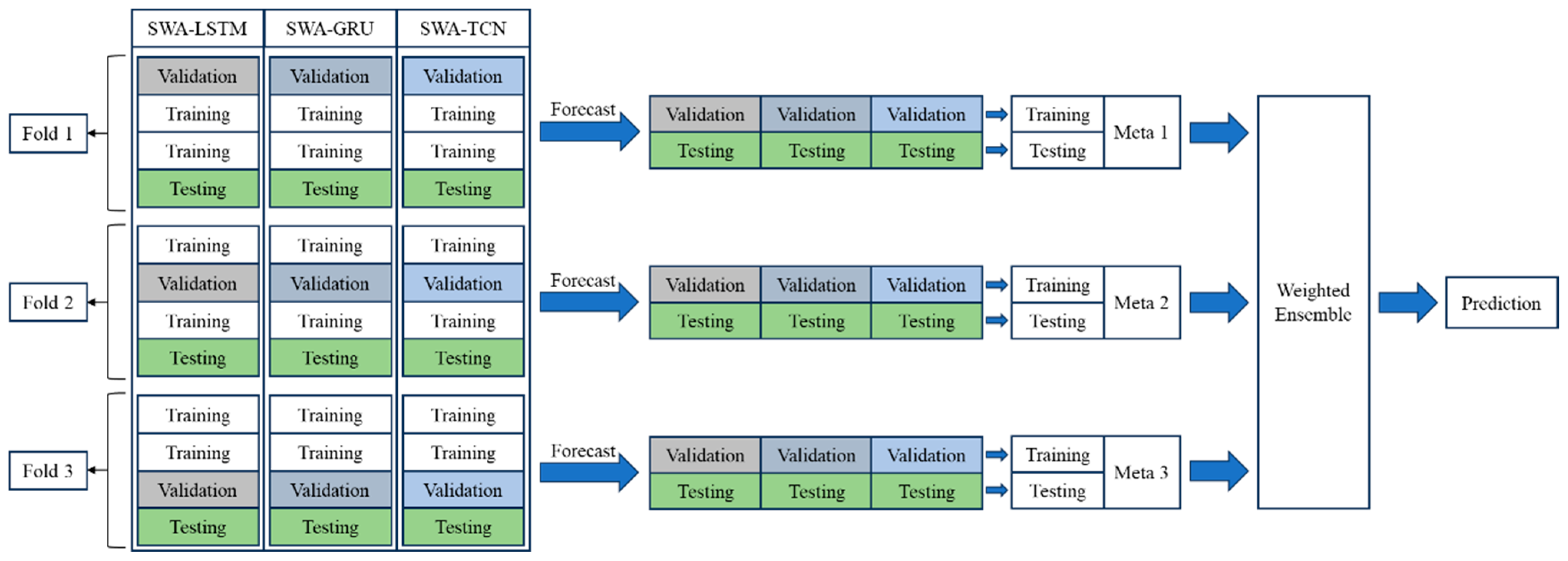
Use K-fold cross-validation to process the original data. The original runoff data and other feature data are divided into a training set and a test set. The training set is then divided into k copies on average using K-fold cross-validation, with one of these copies selected as the sub-validation set. The remaining $k-1$ copies are used as the sub-training set, resulting in k groups of different sub-training sets and sub-validation sets. The ratio of each sub-training set and sub-validation set in the same group to the original training set is $\left(k-1\right):1$, with no overlap between the sets.

(4)

Train and predict with the SWA-ensembled base models. For each fold, the SWA-ensembled base models obtained from step (2) are trained on the K-fold cross-validation sub-training sets and used to predict the sub-validation and test sets. Each base model is trained and predicted k times, independently, to generate the sub-validation and test set predictions for each fold.

(5)

Train and predict with the meta models in the FWWS method. The prediction results of the sub-validation set and test set of multiple basic models on each fold are horizontally spliced and used as the training set and test set of the meta model. After training, the meta model is used to predict its training and test sets. A total of k meta models are trained, yielding k sets of predictions for both the training and test sets.

(6)

Construct the multi-scale ensemble model based on SWA and Fold-Wise Weighted Stacking. According to the root mean square error (RMSE) of the prediction results of k meta models on their training sets, the weights were assigned to each meta model by Equation (13), and the multi-scale ensemble model based on SWA and Fold-Wise Weighted Stacking was constructed.

$$w_l={\displaystyle \frac{\frac{1}{M_{R,l}}}{\sum _{i=0}^k\frac{1}{M_{R,i}}}}$$

(13)

where $w_l$ is the weight of the l-th meta model, $l=1,2,\dots ,k$; $M_{R,l}$ is the RMSE of the l-th meta model, and $M_{R,i}$ is the RMSE of the i-th meta model.

The final prediction result of the SWA–FWWS model $S$ is:

$$S={{w_1·S_1+w}_2·S_2+\dots +w}_k·S_k$$

(14)

where $S_k$ is the prediction result of the k-th meta model on the test set.

In this study, we chose LSTM, GRU, and TCN as the initial models and constructed SWA–LSTM, SWA–GRU, and SWA–TCN models as the base models for the FWWS method using the SWA approach. LightGBM was used as the meta model for FWWS. To improve prediction efficiency, we used 3-fold cross-validation to split the sub-training and sub-validation sets for each base model. The prediction results of the three meta models are finally integrated as the final prediction results. The workflow of the SWA–FWWS model for monthly runoff prediction is shown in Figure 4.

2.4. Evaluation Metrics

In this study, the root mean square error (RMSE), correlation coefficient (r), and Nash–Sutcliffe efficiency (NSE) are selected as the evaluation metrics for model performance. The RMSE metric evaluates the precision of a model’s predictions by computing the square root of the average of squared deviations between forecasted and observed values. A lower RMSE score signifies superior predictive capability, while a larger RMSE suggests poorer accuracy. The r assesses whether the model successfully captures the main trends and directions of runoff variation; the closer r is to 1, the better the model’s fit. NSE measures predictive efficiency by comparing the variance of model-predicted values to that of observed values. These metrics not only comprehensively evaluate the accuracy, robustness, and strength of the linear relationship and fit of the model, but also provide an important basis for model optimization and selection, helping to improve the accuracy and reliability of monthly runoff predictions. The formulas for these evaluation metrics are shown below.

$$RMSE=\sqrt{{\displaystyle \frac{1}{N}}\sum _{i=1}^N{\left(y_i-{\widehat{y}}_i\right)}^2}$$

(15)

$$r={\displaystyle \frac{{\sum }_{i=1}^N\left(y_i-{\overline{y}}_i\right)\left({\widehat{y}}_i-\overline{{\widehat{y}}_i}\right)}{\sqrt{\sum _{i=1}^N{\left(y_i-{\overline{y}}_i\right)}^2\sum _{i=1}^N{\left({\widehat{y}}_i-\overline{{\widehat{y}}_i}\right)}^2}}}$$

(16)

$$NSE=1-{\displaystyle \frac{\sum _{i=1}^N(y_i-{\widehat{y}}_i{)}^2}{\sum _{i=1}^N(y_i-{\overline{y}}_i{)}^2}}$$

(17)

where $y_i$ and ${\overline{y}}_i$ represent the actual monthly runoff values and their mean, respectively, and ${\widehat{y}}_i$ and $\overline{{\widehat{y}}_i}$ represent the predicted monthly runoff values and their mean.

In addition to these commonly used performance metrics, this study further evaluates the model’s performance by decomposing RMSE into three components: Bias, amplitude error (${SD}_{bias}$), and phase error (DISP), providing a more in-depth assessment of model performance [57]. Bias indicates the systematic error of the model, i.e., whether the model systematically overestimates or underestimates the predicted values on average; the closer the bias is to zero, the smaller the systematic error. ${SD}_{bias}$ bias reflects the model‘s ability to capture the variability in the data; the closer the amplitude error is to zero, the more accurately the model captures the fluctuations in the data. DISP measures the temporal alignment between the predicted and actual values; the smaller the DISP, the more synchronized the predicted and actual values are. The mathematical expressions are as follows:

$${RMSE}^2={Bias}^2{+SD}_{bias}^2+{DISP}^2$$

(18)

$$Bias={\displaystyle \frac{1}{N}}{\sum }_{i=1}^N({\widehat{y}}_i-y_i)$$

(19)

$${SD}_{bias}={\sigma }_T+{\sigma }_P$$

(20)

$$DISP=\sqrt{{2\sigma }_T{\sigma }_P(1-R_{TP})}$$

(21)

where ${\sigma }_T$ is the standard deviation of the actual monthly runoff, ${\sigma }_P$ is the standard deviation of the predicted monthly runoff, and $R_{TP}$ is the cross-correlation coefficient between the actual and predicted monthly runoff values.

3. Case Study

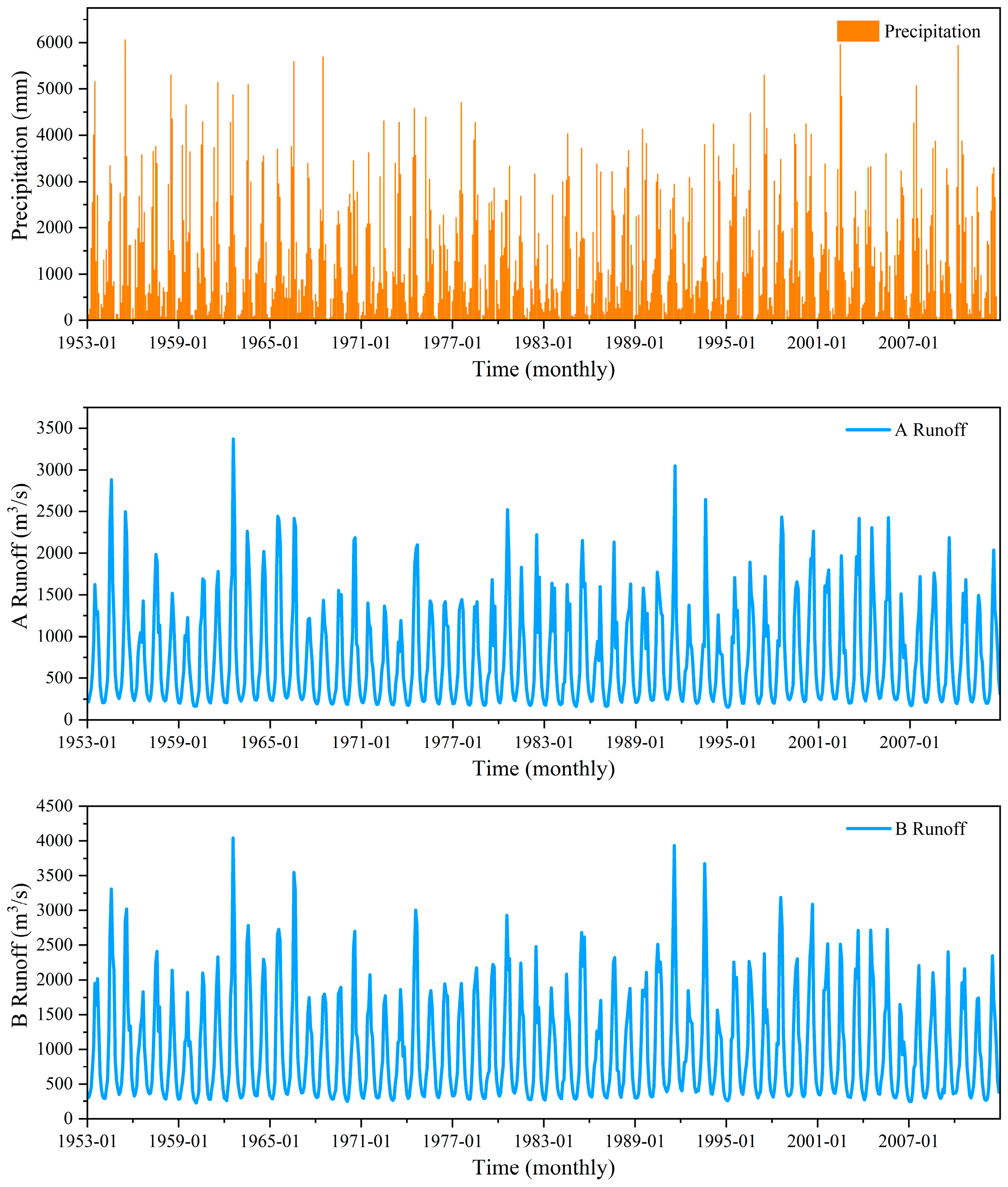
3.1. Study Data

This study focuses on Reservoir A (upstream) and Reservoir B (downstream) in a river. The selected dataset spans from January 1953 to December 2012, including the monthly average runoff of both reservoirs and the total monthly precipitation of the basin of the river. The original monthly runoff series of Reservoir A and Reservoir B, along with the total monthly precipitation in the basin, are shown in Figure 5. Both the runoff and meteorological data were obtained from the local hydrological bureau.

3.2. Data Preprocessing

In this study, monthly total precipitation and historical runoff data from the basin are used as inputs to predict the future runoff. Based on the autocorrelation analysis of monthly runoff and the cross-correlation analysis of monthly total precipitation, runoff with a 12-month lag and monthly total precipitation with a lag of 12 months were selected as model inputs to predict the inflow runoff for the following month.

Data from January 1953 to December 1997 at each station were used as the training set, and data from January 1998 to December 2012 were used as the test set for model parameter training and performance evaluation. In addition, before feeding the data into the model, normalization was applied to improve the model‘s learning and processing efficiency. The normalization formula is as follows:

$$R_{\mathit{norm}}={\displaystyle \frac{R-R_{\mathit{min}}}{R_{\mathit{max}}-R_{\mathit{min}}}}$$

(22)

where $R_{\mathrm{norm}}$ represents the normalized data, $R$ is the original data, and $R_{\max }$ and $R_{\mathrm{m}\mathrm{in}}$ are the maximum and minimum values in the original data, respectively.

3.3. Comparative Experiment Design

To demonstrate the effectiveness and reliability of the proposed FWWS model and the SWA–FWWS combination model in runoff prediction for the river, this section presents a comparison with traditional deep learning models (LSTM, GRU, and TCN) as well as popular ensemble models such as Blending and Stacking. The comparative experiment design was as follows:

(1)

The SWA-ensembled deep learning models (SWA–LSTM, SWA–GRU, SWA–TCN) were compared with their respective non-ensembled base models (LSTM, GRU, TCN) to demonstrate the optimization performance of the SWA method on these three models.

(2)

To ensure consistency in the structure of the base and meta models across ensemble models, trained LSTM, GRU, and TCN models were chosen as the base models for all ensemble models, and LightGBM is selected as the meta model. The proposed FWWS model is compared with the novel Blending model and the traditional Stacking model.

(3)

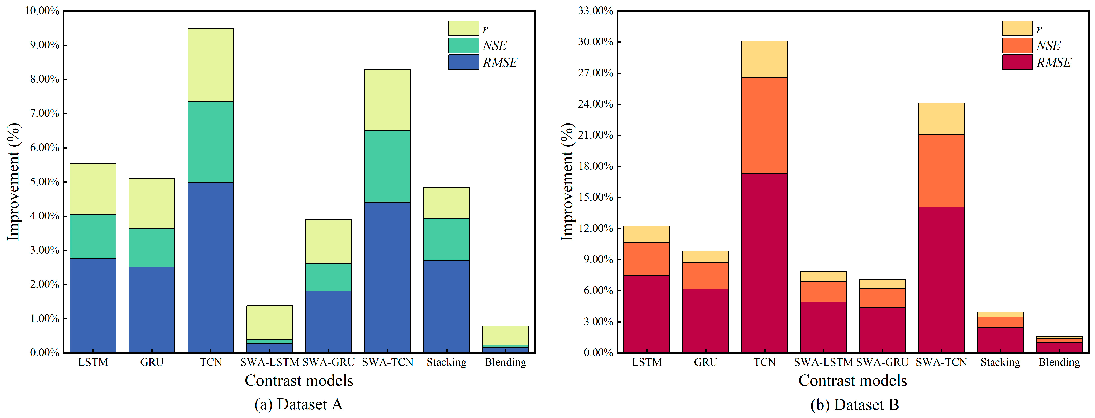
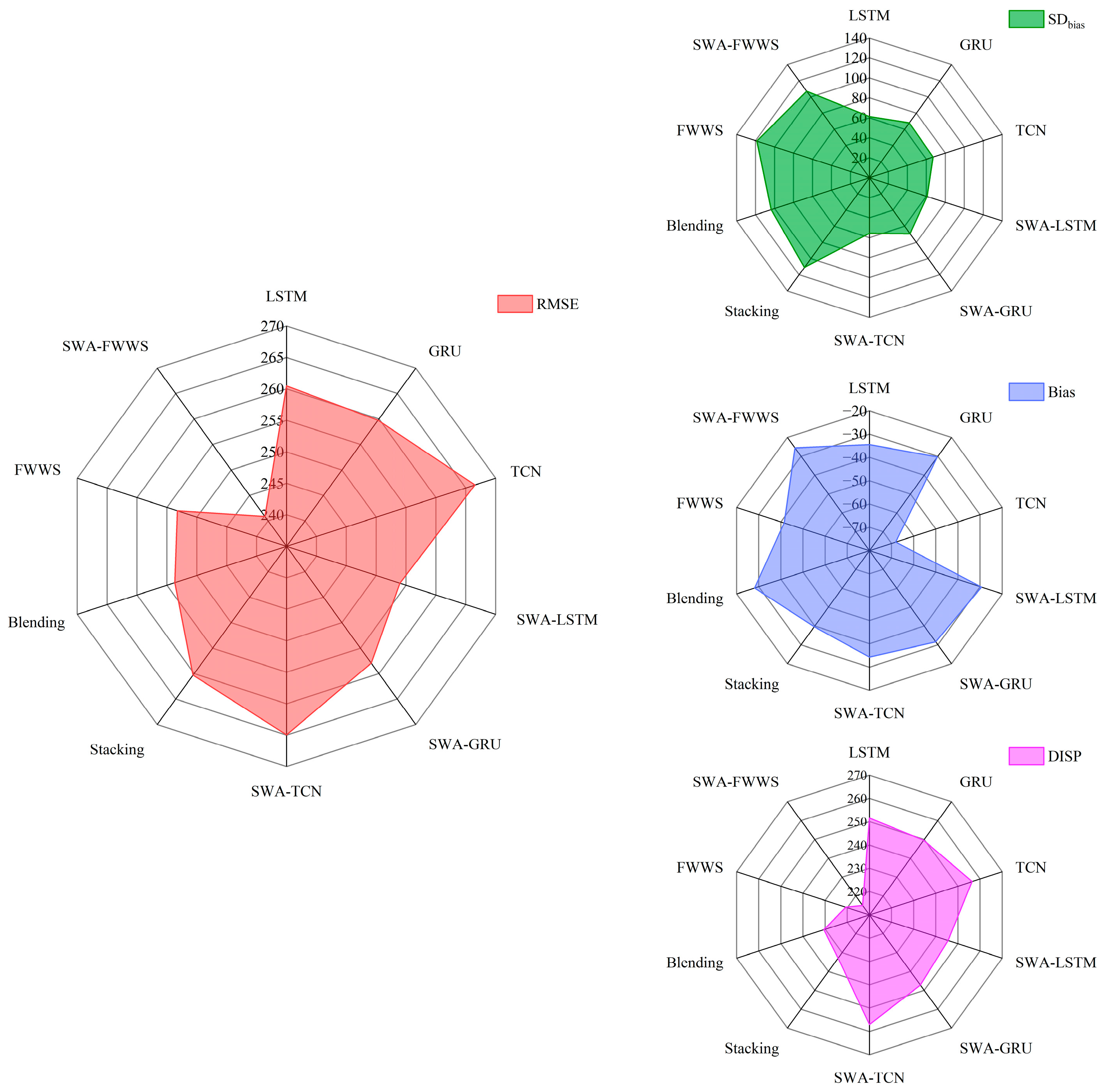
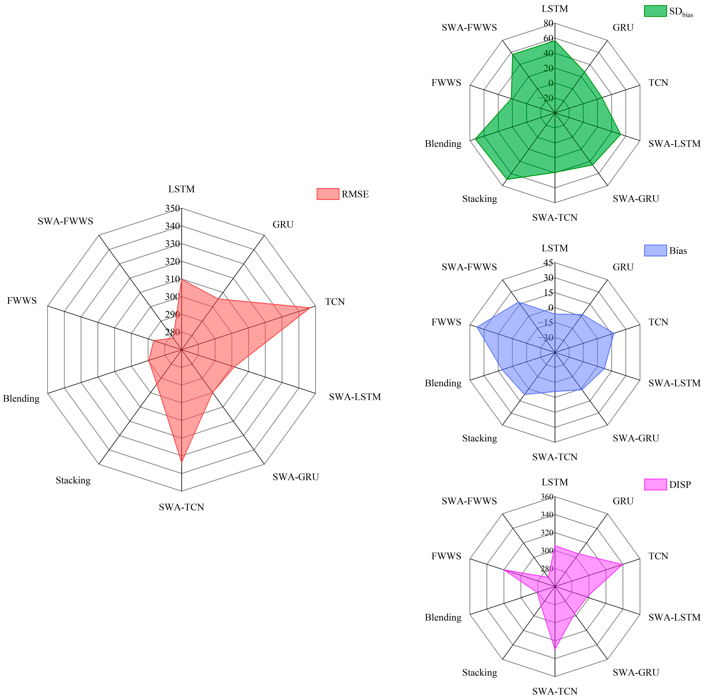
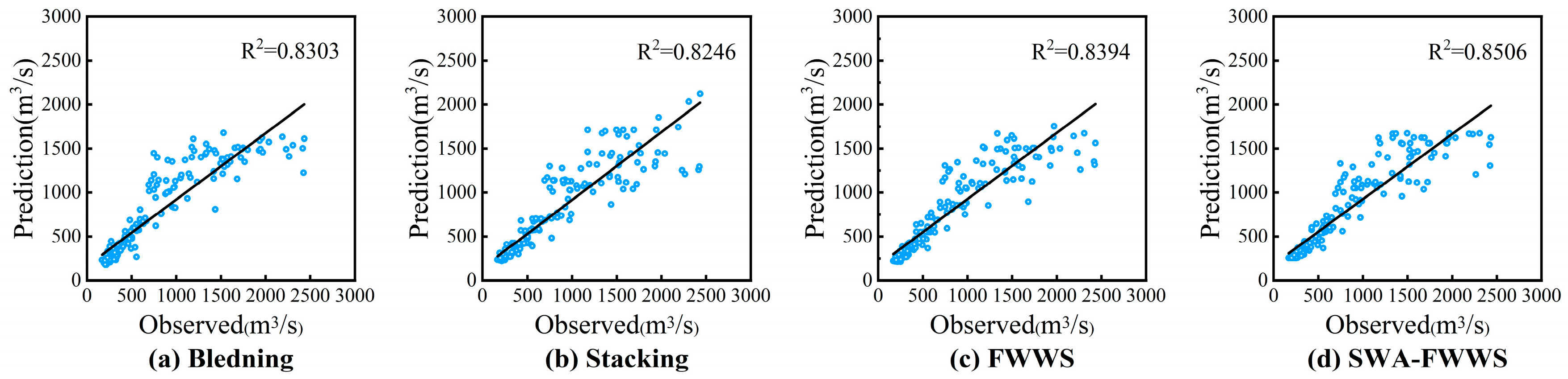
To further improve the prediction performance of the FWWS model regarding runoff in the river, the trained SWA–LSTM, SWA–GRU, and SWA–TCN models were used as base models in the FWWS framework, forming the SWA–FWWS model for monthly runoff prediction. By comparing it with other ensemble models, the superiority of the proposed SWA–FWWS model is demonstrated from multiple aspects.

In this study, the upper and lower bounds of the learning rate for the SWA algorithm are set to 0.006 and 0.0006, respectively. The cosine annealing learning rate adjustment starts from the 360th epoch, with a cycle of eight epochs, repeated five times until the model completes training at the 400th epoch. The Adam optimizer is used to optimize the model parameters during training. The hyper-parameters of each model for different study objects are shown in

Table 1. Hyper-parameters of each model.

Study Objects	Models	Hyper-Parameters
A	LSTM	num_layers = 2, learning_rate = 0.006, num_epochs = 400, hidden_size = 10
	GRU	num_layers = 2, learning_rate = 0.006, num_epochs = 400, hidden_size = 6
	TCN	kernel_size = 3, learning_rate = 0.006, num_epochs = 400, num_channels = [10,11]
	SWA–LSTM (LSTM)	Same as LSTM
	SWA–GRU (GRU)	Same as GRU
	SWA–TCN (TCN)	Same as TCN
	LightGBM (Stacking)	min_data_in_leaf = 1, learning_rate = 0.03, max_depth = 5, num_epochs = 102
	LightGBM (Blending)	min_data_in_leaf = 20, learning_rate = 0.1, max_depth = -1, num_epochs = 53
	LightGBM (FWWS)	min_data_in_leaf = 1; 6; 25, learning_rate = 0.03; 0.02; 0.03, max_depth = 5; 4; 4, num_epochs = 174; 193; 183
	LightGBM (SWA–FWWS)	min_data_in_leaf = 24; 4; 30, learning_rate = 0.008; 0.008; 0.008, max_depth = 2; 2; 2, num_epochs = 316; 479; 790
B	LSTM	num_layers = 2, learning_rate = 0.006, num_epochs = 400, hidden_size = 18
	GRU	num_layers = 2, learning_rate = 0.006, num_epochs = 400, hidden_size = 14
	TCN	kernel_size = 3, learning_rate = 0.006, num_epochs = 400, num_channels = [12,13]
	SWA–LSTM (LSTM)	Same as LSTM
	SWA–GRU (GRU)	Same as GRU
	SWA–TCN (TCN)	Same as TCN
	LightGBM (Stacking)	min_data_in_leaf = 5, learning_rate = 0.009, max_depth = 3, num_epochs = 46
	LightGBM (Blending)	min_data_in_leaf = 8, learning_rate = 0.09, max_depth = 3, num_epochs = 75
	LightGBM (FWWS)	min_data_in_leaf = 5; 8; 7, learning_rate = 0.058; 0.07; 0.03, max_depth = 3; 4; 3, num_epochs = 157; 53; 168
	LightGBM (SWA–FWWS)	min_data_in_leaf = 1; 8; 20, learning_rate = 0.01; 0.05; 0.01, max_depth = 2; 2; −1, num_epochs = 473; 108; 277

Note: Since the base models for the Stacking, Blending, FWWS, and SWA–FWWS models are already trained LSTM, GRU, SWA–LSTM, and other models, only the hyperparameter settings for LightGBM, as the meta model, are listed in Table 1.

.

4. Results

To verify the performance of the proposed FWWS model and the ensembled SWA–FWWS model as predictors of river runoff, a comparative analysis was conducted against other ensemble models constructed by multi-model ensemble methods (Stacking, Blending) using the same base models (LSTM, GRU, TCN). The prediction performance of the models was tested on monthly runoff datasets from the A and B reservoirs in the river. RMSE, NSE, and r were used as metrics to evaluate the predictive performance of the models. The results are presented in

Table 2. Performance evaluation results of all models on the A dataset.

Models	RMSE (m3/s)	NSE	r
LSTM	260.4761	0.8114	0.9026
GRU	259.7689	0.8125	0.9029
TCN	266.5296	0.8026	0.8972
SWA–LSTM	253.9630	0.8207	0.9073
SWA–GRU	257.9381	0.8151	0.9046
SWA–TCN	264.9530	0.8049	0.9001
Stacking	260.3061	0.8117	0.9080
Blending	253.6829	0.8211	0.9112
FWWS	253.2615	0.8217	0.9162
SWA–FWWS	240.8563	0.8388	0.9223

and

Table 3. Performance evaluation results of all models on the B dataset.

Models	RMSE (m3/s)	NSE	r
LSTM	309.7994	0.8186	0.9050
GRU	305.4442	0.8236	0.9091
TCN	346.6903	0.7728	0.8883
SWA–LSTM	301.4458	0.8282	0.9103
SWA–GRU	299.8995	0.8300	0.9114
SWA–TCN	333.6082	0.7896	0.8919
Stacking	293.9659	0.8366	0.9148
Blending	289.5780	0.8415	0.9176
FWWS	286.6497	0.8447	0.9193
SWA–FWWS	278.0754	0.8538	0.9243

.

As shown in Table 2, for the monthly runoff prediction of the A Reservoir, the traditional Stacking ensemble model underperformed compared to the GRU model (with the exception of the r metric) in terms of RMSE and NSE. This indicates that the traditional Stacking ensemble model did not effectively improve prediction accuracy by integrating base models. In contrast, the proposed SWA–FWWS model exhibited the best predictive performance across all models, reducing RMSE by 7.47% and 5.06% compared to the traditional Stacking and Blending models, respectively. Furthermore, the proposed FWWS ensemble model also outperformed the traditional Stacking model in all three metrics.

Similarly, as seen in Table 3, the proposed SWA–FWWS model also achieved the best performance in the runoff prediction for the B Reservoir, with an RMSE of 278.0754, NSE of 0.8538, and r of 0.9243. The proposed FWWS ensemble model also improved RMSE, NSE, and r by 2.49%, 0.97%, and 0.49%, respectively, compared to the traditional Stacking model. Additionally, among the individual model results, the three SWA-ensembled models—SWA–LSTM, SWA–GRU, and SWA–TCN—constructed by ensembling the SWA method with deep learning models, improved RMSE, NSE, and r by 2.76%, 1.37%, and 0.41%, respectively, compared to their original counterparts.

Figure 6 and Figure 7 illustrate the improvements of the FWWS and SWA–FWWS models compared to other models of monthly runoff prediction. The figures clearly show that both the improved Stacking model (FWWS) and its multi-scale ensemble model using the SWA technique (SWA–FWWS) demonstrated significant enhancements in runoff prediction for the river, surpassing other models.

In summary, the proposed SWA–FWWS and FWWS models outperformed other individual and ensemble models in predicting monthly runoff for the river across all evaluation metrics, demonstrating superior accuracy, adaptability, and robustness.

To further analyze the performance of the SWA–FWWS model in monthly runoff forecasting for the river, the RMSE metric was decomposed into more detailed forecasting evaluation indicators: Bias, standard deviation bias (${SD}_{bias}$), and phase error (DISP). The evaluation results of each model for the A and B datasets are shown in Figure 8 and Figure 9.

Overall, the proposed SWA–FWWS model performed best in terms of RMSE. In the ${SD}_{bias}$ metric, which reflects the ability to predict the amplitude of data fluctuations, all ensemble models showed smaller ${SD}_{bias}$ values compared to individual models, indicating that ensemble models generally performed less well in capturing data volatility. However, from the ${SD}_{bias}$ results, the SWA–FWWS model showed a relative reduction in amplitude error compared to other ensemble models. In terms of the Bias metric, the proposed SWA–FWWS model exhibited optimal performance on the A dataset. However, its performance on the B dataset was less satisfactory, with a relatively high Bias value indicating that the model’s predictions on the B dataset tended to be, on average, higher than the actual values. As can be seen from Figure 8 and Figure 9, the FWWS ensemble model with LSTM, GRU and TCN (poor performance) models as the base model performs worse on both datasets than the SWA–FWWS model with the better performance SWA–LSTM, SWA–GRU, and SWA–TCN models as the base model. Therefore, we believe that the performance of the base models may affect the performance of the final ensemble model on the Bias indicator to a certain extent. For the DISP metric, which measures the temporal alignment between predicted and actual values, the SWA–FWWS model achieved the best performance on both datasets, indicating that the model can accurately capture the temporal patterns of runoff changes.

In conclusion, the proposed SWA–FWWS model demonstrated superior overall performance in monthly runoff prediction for the river compared to other benchmark models from multiple perspectives, exhibiting strong adaptability and stability.

5. Discussion

From the results, it can be seen that the performance of individual base models in monthly runoff prediction shows significant differences compared to ensemble models, and the proposed SWA–FWWS model achieves the best performance in river runoff prediction. To better illustrate the performance of the SWA–FWWS model, this section presents scatter plots to discuss the advantages and disadvantages of the SWA–FWWS model and other ensemble models from the perspective of multi-model ensembles. Figure 10 and Figure 11 depict the scatter plots of the predicted results versus the observed values of the four ensemble models on the A and B test sets, respectively.

The scatter plots of the prediction of each ensemble model against the observations show that the performance of the ensemble models other than SWA–FWWS varies considerably between different datasets, indicating that the models are less stable. However, the SWA–FWWS model not only demonstrated the best stability, but the scatter points were also more concentrated, indicating that the errors between the predicted results and the observed values were smaller. Furthermore, the R-Squared between the predicted and observed values of the proposed model was the highest among all models, suggesting that the proposed model is better at capturing the trends in runoff variation than the other ensemble models.

Upon further analysis, it was observed that the prediction errors of all ensemble models increased as the observed values increased, leading to poorer performance in terms of the ${SD}_{bias}$ metric. This suggests that ensemble models generally struggle with predicting the magnitude of fluctuations in the data, likely due to the limited amount of training data available, which restricted the ability of the ensemble models to adequately learn from larger runoff data.

6. Conclusions

In order to improve the accuracy of monthly runoff prediction, this study proposes a Fold-Wise Weighted Stacking ensemble learning model (SWA–FWWS). This model solves the problem of the lack of correlation between different models in K-fold cross-validation of the traditional Stacking method, and improves the prediction accuracy and generalization of the ensemble model by combining the Stochastic Weight Averaging technique with an improved Stacking method (FWWS).

To verify the effectiveness and practicality of the proposed model for monthly runoff prediction, it was compared with nine prediction models of three different types using six progressively detailed evaluation metrics. The models were tested on an actual monthly runoff prediction task for an upstream reservoir and a downstream reservoir within a river basin. The results show that the FWWS ensemble method, which improves on the traditional Stacking method, more effectively leverages the predictive capabilities of base models, significantly enhancing the accuracy of monthly runoff predictions. Furthermore, the final SWA–FWWS model, which incorporates Stochastic Weight Averaging, outperforms all other models in terms of both prediction accuracy and generalization ability.

While the SWA–FWWS model demonstrates excellent performance across multiple evaluation metrics and case studies, it is important to note that ensemble models generally provide more stable predictions when dealing with runoff data, which can exhibit significant fluctuations. Although the SWA–FWWS model alleviates this issue and improves prediction accuracy, future research should explore more suitable base models to address the limitations of ensemble model.

References

- Qin, P.; Xu, H.; Liu, M.; Du, L.; Xiao, C.; Liu, L.; Tarroja, B. Climate change impacts on Three Gorges Reservoir impoundment and hydropower generation. J. Hydrol. 2020, 580, 123922. [Google Scholar] [CrossRef]
- Evsukoff, A.-G.; Cataldi, M.; de Lima, B.-S.-L.-P. A multi-model approach for long-term runoff modeling using rainfall forecasts. Expert Syst. Appl. 2012, 39, 4938–4946. [Google Scholar] [CrossRef]
- Zolfaghari, M.; Golabi, M.-R. Modeling and predicting the electricity production in hydropower using conjunction of wavelet transform, long short-term memory and random forest models. Renew. Energy 2021, 170, 1367–1381. [Google Scholar] [CrossRef]
- Liu, Z.; Mo, L.; Lou, S.; Zhu, Y.; Liu, T. An Ecology-Oriented Single-Multi-Objective Optimal Operation Modeling and Decision-Making Method in the Case of the Ganjiang River. Water 2024, 16, 970. [Google Scholar] [CrossRef]
- Worthington, T.-A.; Brewer, S.-K.; Vieux, B.; Kennen, J. The accuracy of ecological flow metrics derived using a physics-based distributed rainfall—Runoff model in the Great Plains, USA. Ecohydrology 2019, 12, 2090. [Google Scholar] [CrossRef]
- Tian, Y.; Zhao, Y.; Son, S.; Luo, J.; Oh, S.; Wang, Y. A Deep-Learning Ensemble Method to Detect Atmospheric Rivers and Its Application to Projected Changes in Precipitation Regime. J. Geophys. Res. Atmos. 2023, 128, 037041. [Google Scholar] [CrossRef]
- Cloke, H.-L.; Pappenberger, F. Ensemble flood forecasting: A review. J. Hydrol. 2009, 375, 613–626. [Google Scholar] [CrossRef]
- Chen, C.; Jiang, J.; Liao, Z.; Zhou, Y.; Wang, H.; Pei, Q. A short-term flood prediction based on spatial deep learning network: A case study for Xi County, China. J. Hydrol. 2022, 607, 127535. [Google Scholar] [CrossRef]
- Man, Y.; Yang, Q.; Shao, J.; Wang, G.; Bai, L.; Xue, Y. Enhanced LSTM Model for Daily Runoff Prediction in the Upper Huai River Basin, China. Engineering 2023, 24, 229–238. [Google Scholar] [CrossRef]
- Sengul, S.; Ispirli, M.-N. Predicting Snowmelt Runoff at the Source of the Mountainous Euphrates River Basin in Turkey for Water Supply and Flood Control Issues Using HEC-HMS Modeling. Water 2022, 14, 284. [Google Scholar] [CrossRef]
- Brown, C.-M.; Lund, J.-R.; Cai, X.; Reed, P.-M.; Zagona, E.-A.; Ostfeld, A.; Hall, J.; Characklis, G.-W.; Yu, W.; Brekke, L. The future of water resources systems analysis: Toward a scientific framework for sustainable water management. Water Resour. Res. 2015, 51, 6110–6124. [Google Scholar] [CrossRef]
- Zang, S.; Li, Z.; Zhang, K.; Yao, C.; Liu, Z.; Wang, J.; Huang, Y.; Wang, S. Improving the flood prediction capability of the Xin’anjiang model by formulating a new physics-based routing framework and a key routing parameter estimation method. J. Hydrol. 2021, 603, 126867. [Google Scholar] [CrossRef]
- Yu, W.; Nakakita, E.; Kim, S.; Yamaguchi, K. Improvement of rainfall and flood forecasts by blending ensemble NWP rainfall with radar prediction considering orographic rainfall. J. Hydrol. 2015, 531, 494–507. [Google Scholar] [CrossRef]
- Avila, L.; Silveira, R.; Campos, A.; Rogiski, N.; Freitas, C.; Aver, C.; Fan, F. Seasonal Streamflow Forecast in the Tocantins River Basin, Brazil: An Evaluation of ECMWF-SEAS5 with Multiple Conceptual Hydrological Models. Water 2023, 15, 1695. [Google Scholar] [CrossRef]
- Li, Y.; Wei, J.; Sun, Q.; Huang, C. Research on Coupling Knowledge Embedding and Data-Driven Deep Learning Models for Runoff Prediction. Water 2024, 16, 2130. [Google Scholar] [CrossRef]
- Sheng, Z.; Wen, S.; Feng, Z.; Gong, J.; Shi, K.; Guo, Z.; Yang, Y.; Huang, T. A Survey on Data-Driven Runoff Forecasting Models Based on Neural Networks. IEEE Trans. Emerg. Top. Comput. Intell. 2023, 7, 1083–1097. [Google Scholar] [CrossRef]
- Feng, Z.; Niu, W.; Tang, Z.; Jiang, Z.; Xu, Y.; Liu, Y.; Zhang, H. Monthly runoff time series prediction by variational mode decomposition and support vector machine based on quantum-behaved particle swarm optimization. J. Hydrol. 2020, 583, 124627. [Google Scholar] [CrossRef]
- Wang, W.; Xu, D.; Chau, K.; Chen, S. Improved annual rainfall-runoff forecasting using PSO-SVM model based on EEMD. J. Hydroinform. 2013, 15, 1377–1390. [Google Scholar] [CrossRef]
- Dong, J.; Wang, Z.; Wu, J.; Cui, X.; Pei, R. A Novel Runoff Prediction Model Based on Support Vector Machine and Gate Recurrent unit with Secondary Mode Decomposition. Water Resour. Manag. 2024, 38, 1655–1674. [Google Scholar] [CrossRef]
- Guo, Z.; Zhang, Q.; Li, N.; Zhai, Y.; Teng, W.; Liu, S.; Ying, G. Runoff time series prediction based on hybrid models of two-stage signal decomposition methods and LSTM for the Pearl River in China. Hydrol. Res. 2023, 54, 1505–1521. [Google Scholar] [CrossRef]
- Sun, N.; Zhang, S.; Peng, T.; Zhang, N.; Zhou, J.; Zhang, H. Multi-Variables-Driven Model Based on Random Forest and Gaussian Process Regression for Monthly Streamflow Forecasting. Water 2022, 14, 1828. [Google Scholar] [CrossRef]
- Woodson, D.; Rajagopalan, B.; Zagona, E. Long-Lead Forecasting of Runoff Season Flows in the Colorado River Basin Using a Random Forest Approach. J. Water Res. Plan. Manag. 2024, 150, 6167. [Google Scholar] [CrossRef]
- Chen, S.-J.; Wei, Q.; Zhu, Y.-M.; Ma, G.-W.; Han, X.-Y.; Wang, L. Medium- and long-term runoff forecasting based on a random forest regression model. Water Supply 2020, 20, 3658–3664. [Google Scholar]
- Wu, J.; Wang, Z.; Dong, J.; Cui, X.; Tao, S.; Chen, X. Robust Runoff Prediction with Explainable Artificial Intelligence and Meteorological Variables from Deep Learning Ensemble Model. Water Resour. Res. 2023, 59, 035676. [Google Scholar] [CrossRef]
- Contreras, P.; Orellana-Alvear, J.; Munoz, P.; Bendix, J.; Celleri, R. Influence of Random Forest Hyperparameterization on Short-Term Runoff Forecasting in an Andean Mountain Catchment. Atmosphere 2021, 12, 238. [Google Scholar] [CrossRef]
- Zhang, J.; Xiao, H.; Fang, H. Component-Based Reconstruction Prediction of Runoff at Multi-time Scales in the Source Area of the Yellow River Based on the ARMA Model. Water Resour. Manag. 2022, 36, 433–448. [Google Scholar] [CrossRef]
- Khazaeiathar, M.; Hadizadeh, R.; Attar, N.-F.; Schmalz, B. Daily Streamflow Time Series Modeling by Using a Periodic Autoregressive Model (ARMA) Based on Fuzzy Clustering. Water 2022, 14, 3932. [Google Scholar] [CrossRef]
- Chai, Q.; Zhang, S.; Tian, Q.; Yang, C.; Guo, L. Daily Runoff Prediction Based on FA-LSTM Model. Water 2024, 16, 2216. [Google Scholar] [CrossRef]
- Gao, S.; Huang, Y.; Zhang, S.; Han, J.; Wang, G.; Zhang, M.; Lin, Q. Short-term runoff prediction with GRU and LSTM networks without requiring time step optimization during sample generation. J. Hydrol. 2020, 589, 125188. [Google Scholar] [CrossRef]
- Shrestha, S.-G.; Pradhanang, S.-M. Performance of LSTM over SWAT in Rainfall-Runoff Modeling in a Small, Forested Watershed: A Case Study of Cork Brook, RI. Water 2023, 15, 4194. [Google Scholar] [CrossRef]
- Li, P.; Zhang, J.; Krebs, P. Prediction of Flow Based on a CNN-LSTM Combined Deep Learning Approach. Water 2022, 14, 993. [Google Scholar] [CrossRef]
- Frame, J.-M.; Kratzert, F.; Klotz, D.; Gauch, M.; Shalev, G.; Gilon, O.; Qualls, L.-M.; Gupta, H.; Nearing, G.-S. Deep learning rainfall-runoff predictions of extreme events. Hydrol. Earth Syst. Sc. 2022, 26, 3377–3392. [Google Scholar] [CrossRef]
- Samantaray, S.; Das, S.-S.; Sahoo, A.; Satapathy, D.-P. Monthly runoff prediction at Baitarani river basin by support vector machine based on Salp swarm algorithm. Ain Shams Eng. J. 2022, 13, 101732. [Google Scholar] [CrossRef]
- Chen, X.; Huang, J.; Wang, S.; Zhou, G.; Gao, H.; Liu, M.; Yuan, Y.; Zheng, L.; Li, Q.; Qi, H. A New Rainfall-Runoff Model Using Improved LSTM with Attentive Long and Short Lag-Time. Water 2022, 14, 697. [Google Scholar] [CrossRef]
- Li, J.; Qian, K.; Liu, Y.; Yan, W.; Yang, X.; Luo, G.; Ma, X. LSTM-Based Model for Predicting Inland River Runoff in Arid Region: A Case Study on Yarkant River, Northwest China. Water 2022, 14, 1745. [Google Scholar] [CrossRef]
- Zhang, L.; Yang, X. Applying a Multi-Model Ensemble Method for Long-Term Runoff Prediction under Climate Change Scenarios for the Yellow River Basin, China. Water 2018, 10, 301. [Google Scholar] [CrossRef]
- Arsenault, R.; Gatien, P.; Renaud, B.; Brissette, F.; Martel, J. A comparative analysis of 9 multi-model averaging approaches in hydrological continuous streamflow simulation. J. Hydrol. 2015, 529, 754–767. [Google Scholar] [CrossRef]
- Liu, S.; Qin, H.; Liu, G.; Xu, Y.; Zhu, X.; Qi, X. Runoff Forecasting of Machine Learning Model Based on Selective Ensemble. Water Resour. Manag. 2023, 37, 4459–4473. [Google Scholar] [CrossRef]
- Yao, J.; Zhang, X.; Luo, W.; Liu, C.; Ren, L. Applications of Stacking/Blending ensemble learning approaches for evaluating flash flood susceptibility. Int. J. Appl. Earth Obs. 2022, 112, 102932. [Google Scholar] [CrossRef]
- Zounemat-Kermani, M.; Batelaan, O.; Fadaee, M.; Hinkelmann, R. Ensemble machine learning paradigms in hydrology: A review. J. Hydrol. 2021, 598, 126266. [Google Scholar] [CrossRef]
- Leng, Z.; Chen, L.; Yang, B.; Li, S.; Yi, B. An extreme forecast index-driven runoff prediction approach using stacking ensemble learning. Geomat. Nat. Haz Risk 2024, 15, 2353144. [Google Scholar] [CrossRef]
- Xie, Y.; Sun, W.; Ren, M.; Chen, S.; Huang, Z.; Pan, X. Stacking ensemble learning models for daily runoff prediction using 1D and 2D CNNs. Expert Syst. Appl. 2023, 217, 119469. [Google Scholar] [CrossRef]
- Deb, D.; Arunachalam, V.; Raju, K.-S. Daily reservoir inflow prediction using stacking ensemble of machine learning algorithms. J. Hydroinform. 2024, 26, 972–997. [Google Scholar] [CrossRef]
- Mohammed, A.; Kora, R. A comprehensive review on ensemble deep learning: Opportunities and challenges. J. King Saud. Univ-Com. 2023, 35, 757–774. [Google Scholar] [CrossRef]
- Dong, F.; Javed, A.; Saber, A.; Neumann, A.; Arnillas, C.-A.; Kaltenecker, G.; Arhonditsis, G. A flow-weighted ensemble strategy to assess the impacts of climate change on watershed hydrology. J. Hydrol. 2021, 594, 125898. [Google Scholar] [CrossRef]
- Yao, Z.; Wang, Z.; Wang, D.; Wu, J.; Chen, L. An ensemble CNN-LSTM and GRU adaptive weighting model based improved sparrow search algorithm for predicting runoff using historical meteorological and runoff data as input. J. Hydrol. 2023, 625, 129977. [Google Scholar] [CrossRef]
- Liu, S.; Xu, J.; Zhao, J.; Xie, X.; Zhang, W. Efficiency enhancement of a process-based rainfall—Runoff model using a new modified AdaBoost.RT technique. Appl. Soft Comput. 2014, 23, 521–529. [Google Scholar] [CrossRef]
- Lu, M.; Hou, Q.; Qin, S.; Zhou, L.; Hua, D.; Wang, X.; Cheng, L. A Stacking Ensemble Model of Various Machine Learning Models for Daily Runoff Forecasting. Water 2023, 15, 1265. [Google Scholar] [CrossRef]
- Hochreiter, S.; Schmidhuber, J. Long short-term memory. Neural Comput. 1997, 9, 1735–1780. [Google Scholar] [CrossRef]
- He, S.; Sang, X.; Yin, J.; Zheng, Y.; Chen, H. Short-term Runoff Prediction Optimization Method Based on BGRU-BP and BLSTM-BP Neural Networks. Water Resour. Manag. 2023, 37, 747–768. [Google Scholar] [CrossRef]
- Bai, S.; Kolter, J.-Z.; Koltun, V. An Empirical Evaluation of Generic Convolutional and Recurrent Networks for Sequence Modeling. arXiv 2018, arXiv:1803.01271. [Google Scholar]
- Hewage, P.; Behera, A.; Trovati, M.; Pereira, E.; Ghahremani, M.; Palmieri, F.; Liu, Y. Temporal convolutional neural (TCN) network for an effective weather forecasting using time-series data from the local weather station. Soft Comput. 2020, 24, 16453–16482. [Google Scholar] [CrossRef]
- Fan, J.; Zhang, K.; Huang, Y.; Zhu, Y.; Chen, B. Parallel spatio-temporal attention-based TCN for multivariate time series prediction. Neural Comput. Appl. 2023, 35, 13109–13118. [Google Scholar] [CrossRef]
- Ke, G.; Meng, Q.; Finley, T.; Wang, T.; Chen, W.; Ma, W.; Ye, Q.; Liu, T. LightGBM: A Highly Efficient Gradient Boosting Decision Tree. In Proceedings of the Advances in Neural Information Processing Systems 30 (NIPS 2017), Long Beach, CA, USA, 4–9 December 2017; p. 30. [Google Scholar]
- Izmailov, P.; Podoprikhin, D.; Garipov, T.; Vetrov, D.; Wilson, A.-G. Averaging Weights Leads to Wider Optima and Better Generalization. arXiv 2018, arXiv:1803.05407. [Google Scholar]
- Shen, Q.; Mo, L.; Liu, G.; Zhou, J.; Zhang, Y.; Ren, P. Short-Term Load Forecasting Based on Multi-Scale Ensemble Deep Learning Neural Network. IEEE Access 2023, 11, 111963–111975. [Google Scholar] [CrossRef]
- Yuan, X.; Chen, C.; Lei, X.; Yuan, Y.; Adnan, R.-M. Monthly runoff forecasting based on LSTM-ALO model. Stoch. Environ. Res. Risk Assess. 2018, 32, 2199–2212. [Google Scholar] [CrossRef]