
Advancing SWAT Model Calibration: A U-NSGA-III-Based Framework for Multi-Objective Optimization


Abstract
1. Introduction
2. Methods
2.1. SWAT Model
2.2. U-NSGA-III Algorithm
2.3. Py-SWAT-U-NSGA-III: A Framework for Parallel Calibration of the SWAT Model with U-NSGA-III
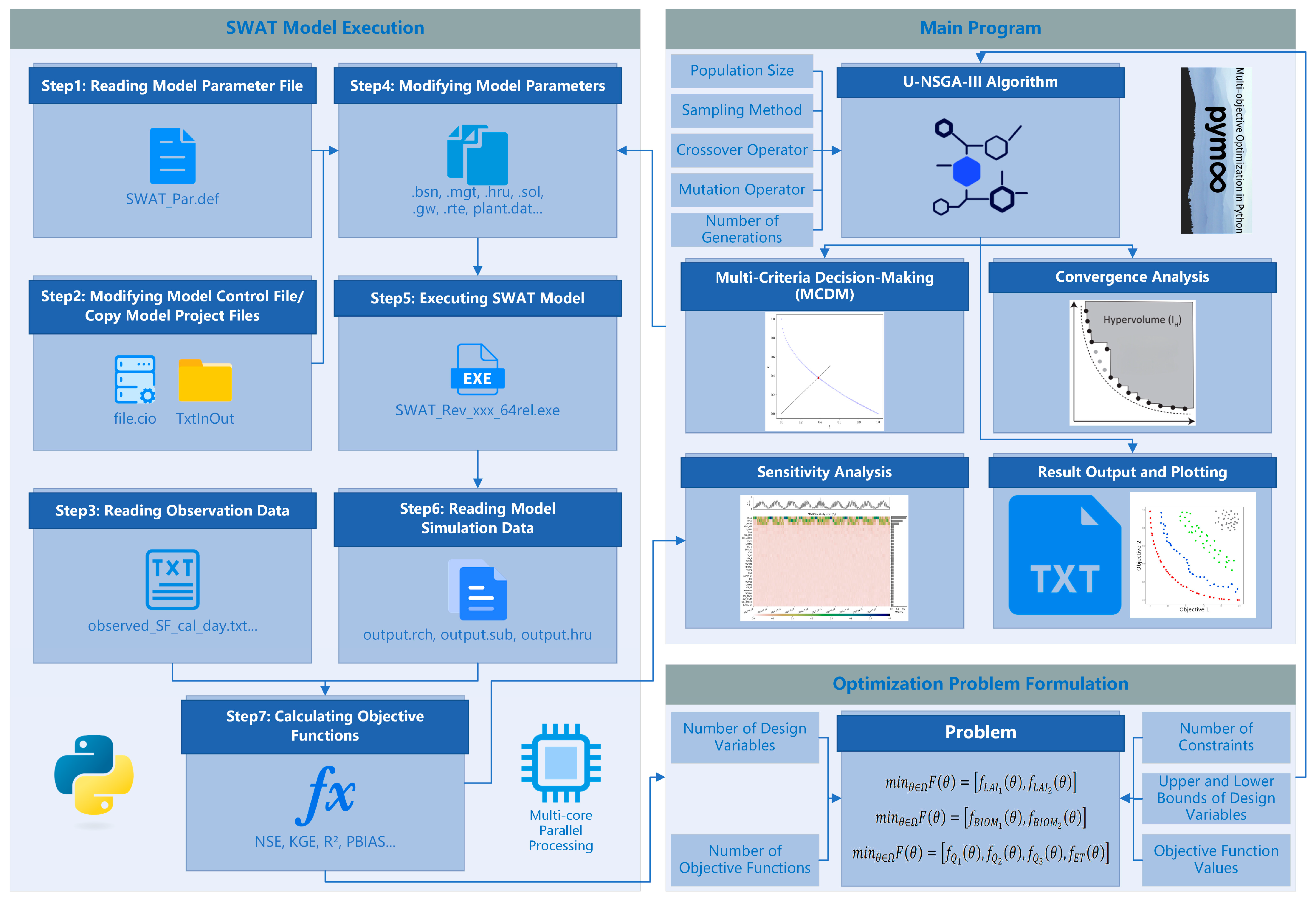
2.3.1. Overall Design
2.3.2. Implementation of the Py-SWAT-U-NSGA-III Framework
- Multi-Criteria Decision Making (MCDM): This is used to obtain the best tradeoff solution after multi-objective optimization, which includes two methods: compromise programming [70] and pseudo-weights [71]. The compromise programming method uses user-defined distance metrics to determine the Pareto optimal solution closest to the reference point; typically, the reference point is the ideal point, representing the best-expected objective function values [13]. Meanwhile, the pseudo-weights method generates a vector for each Pareto optimal solution, representing the relative importance (or weights) of each objective function [13]. The sum of the different weights in each vector is forced to one. In this framework, the compromise programming method is the default option;
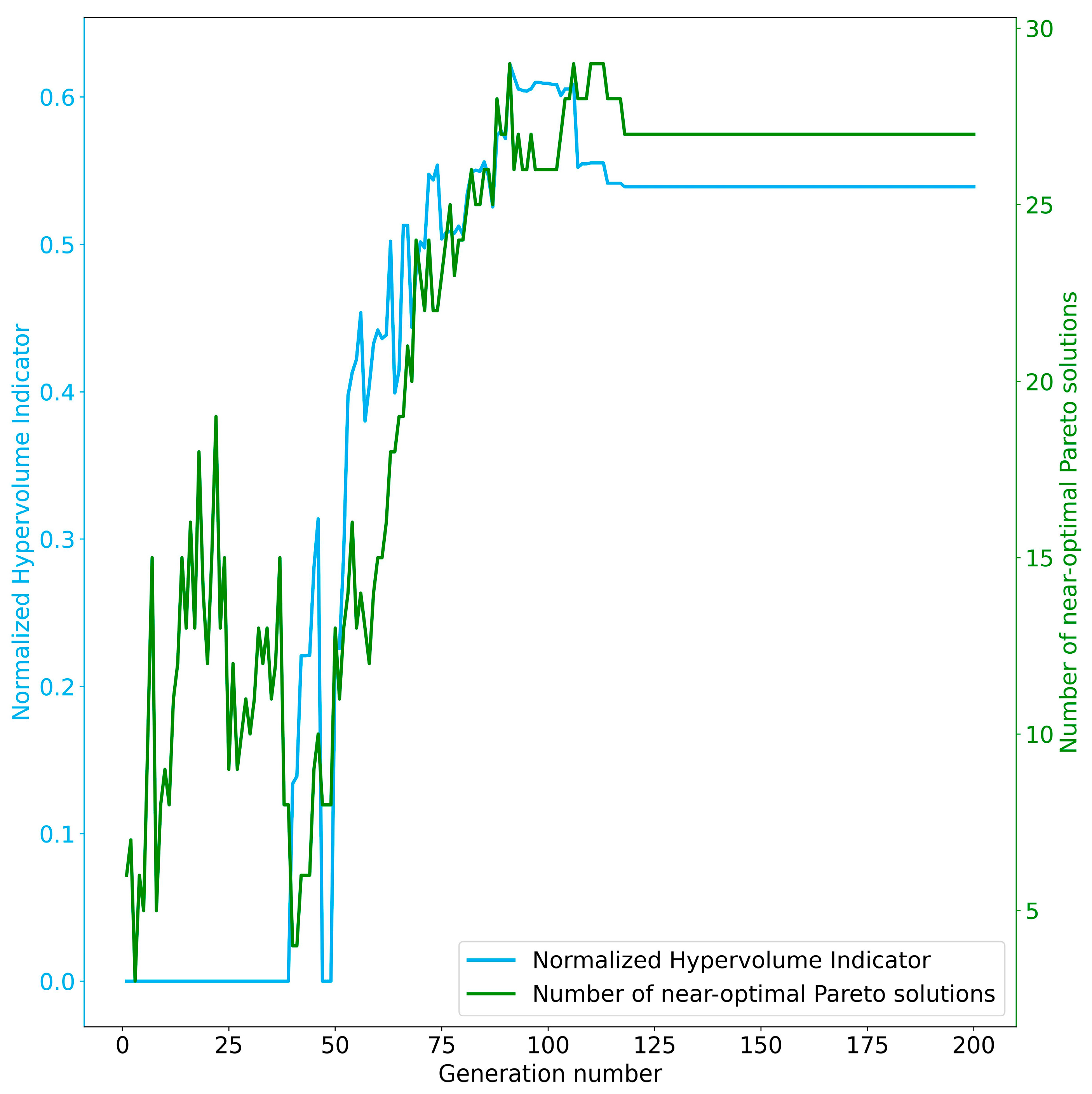
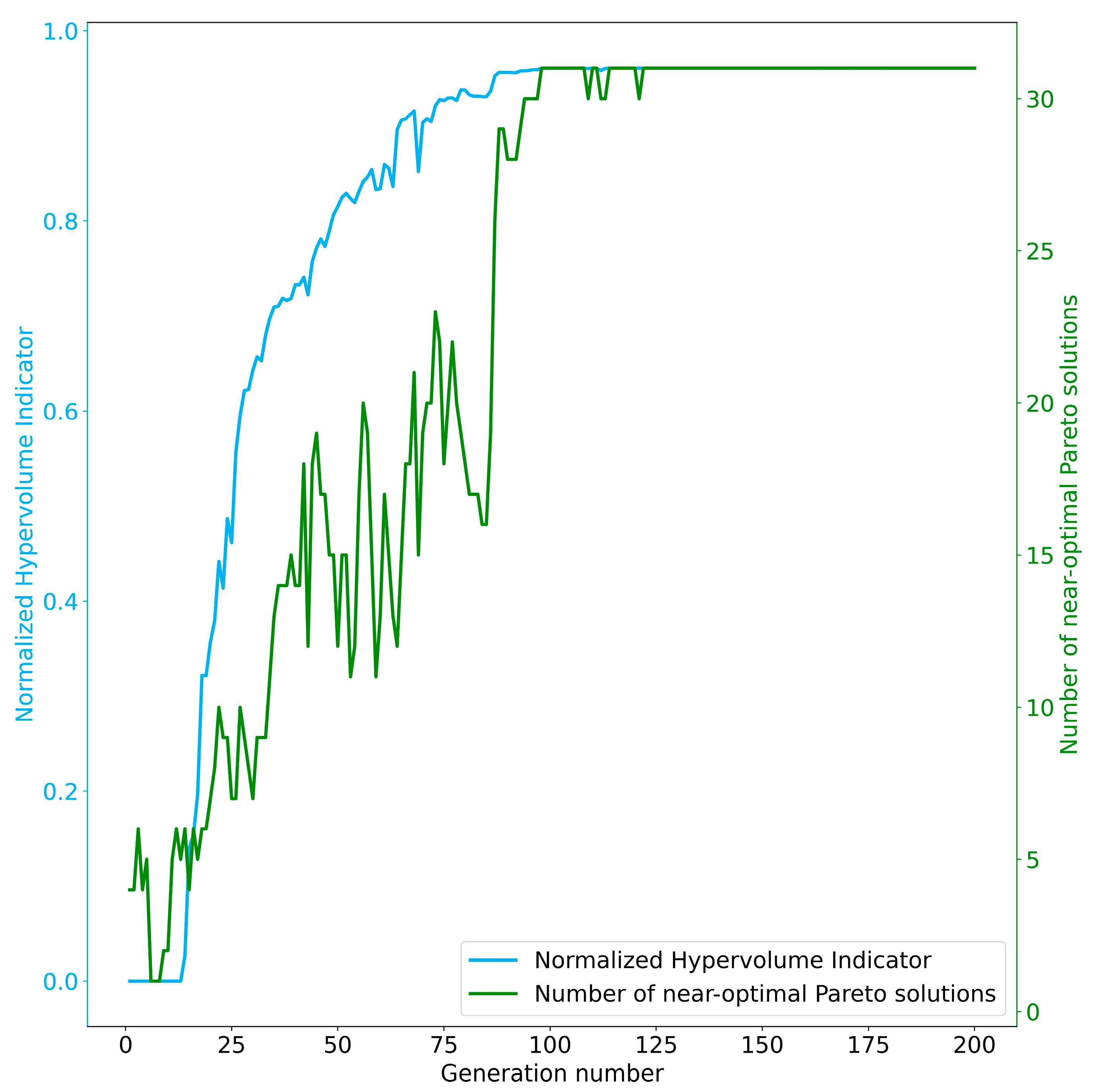
- Convergence Analysis: This employs the hypervolume indicator [72], a commonly used metric for evaluating the approximations of the Pareto front (PF) generated by MOEAs [73]. A higher value of the hypervolume indicator indicates a better solution and the ideal value is one. The definition of the hypervolume indicator, its calculation, and cases in the space of the 2 objective functions are provided in S1 and Figure S1 in the Supplementary Materials;
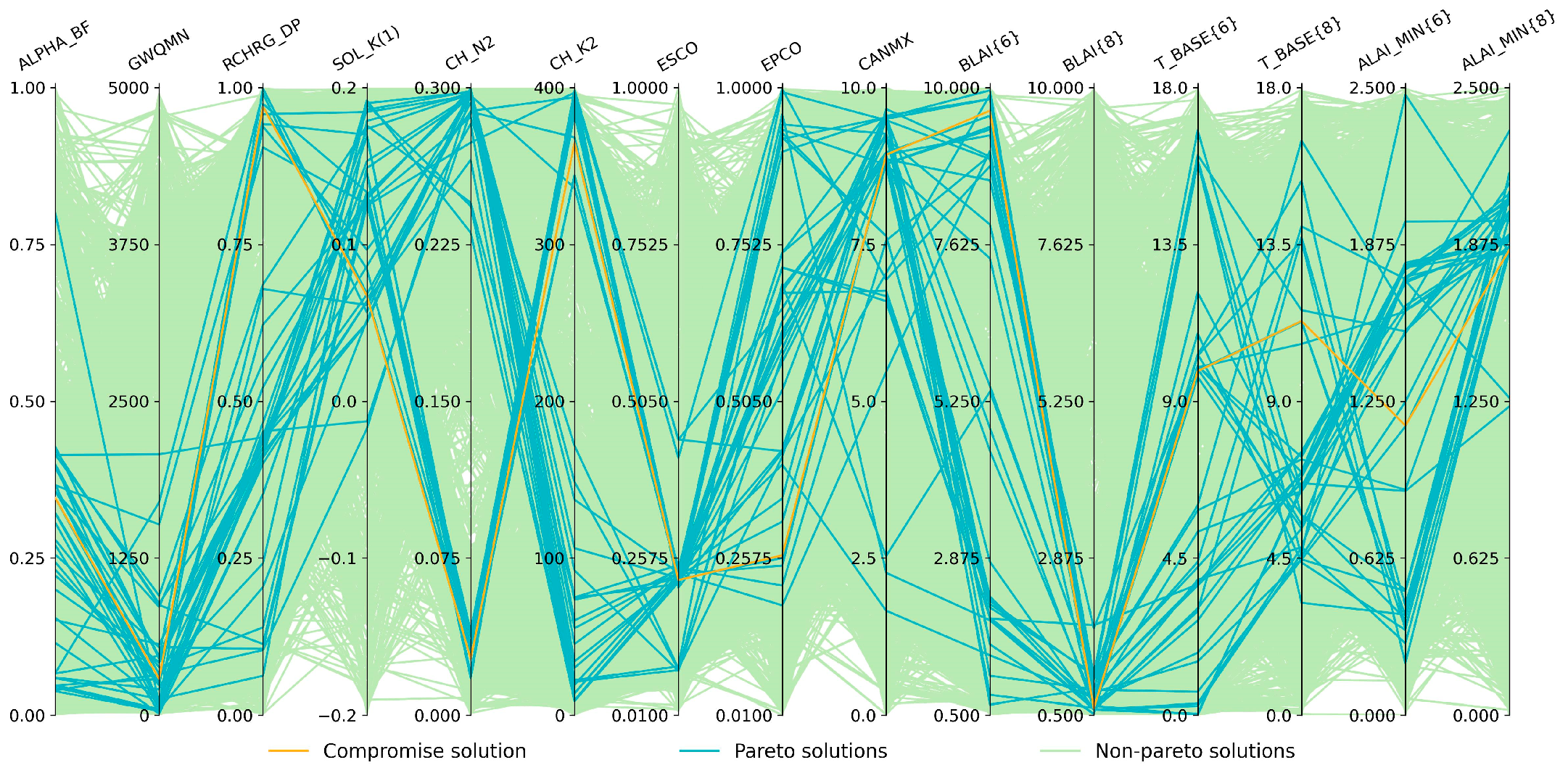
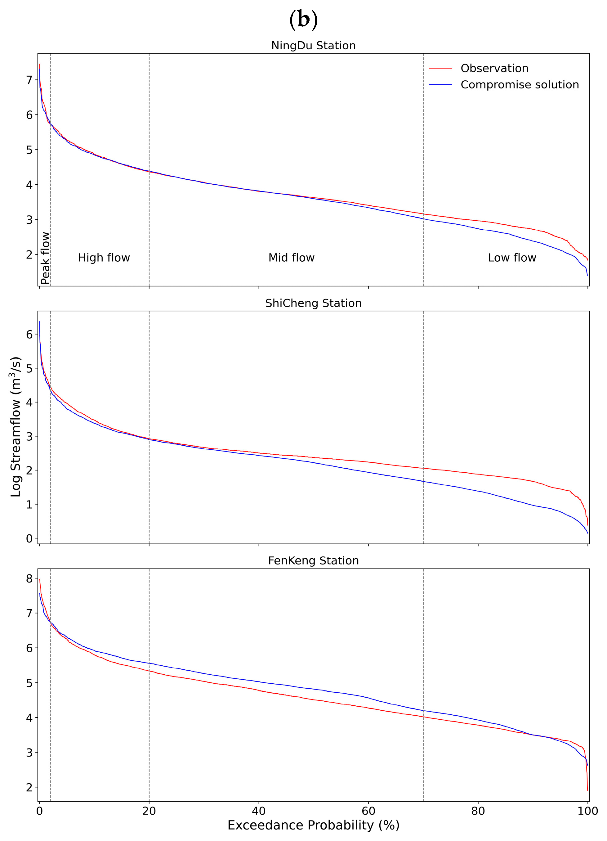
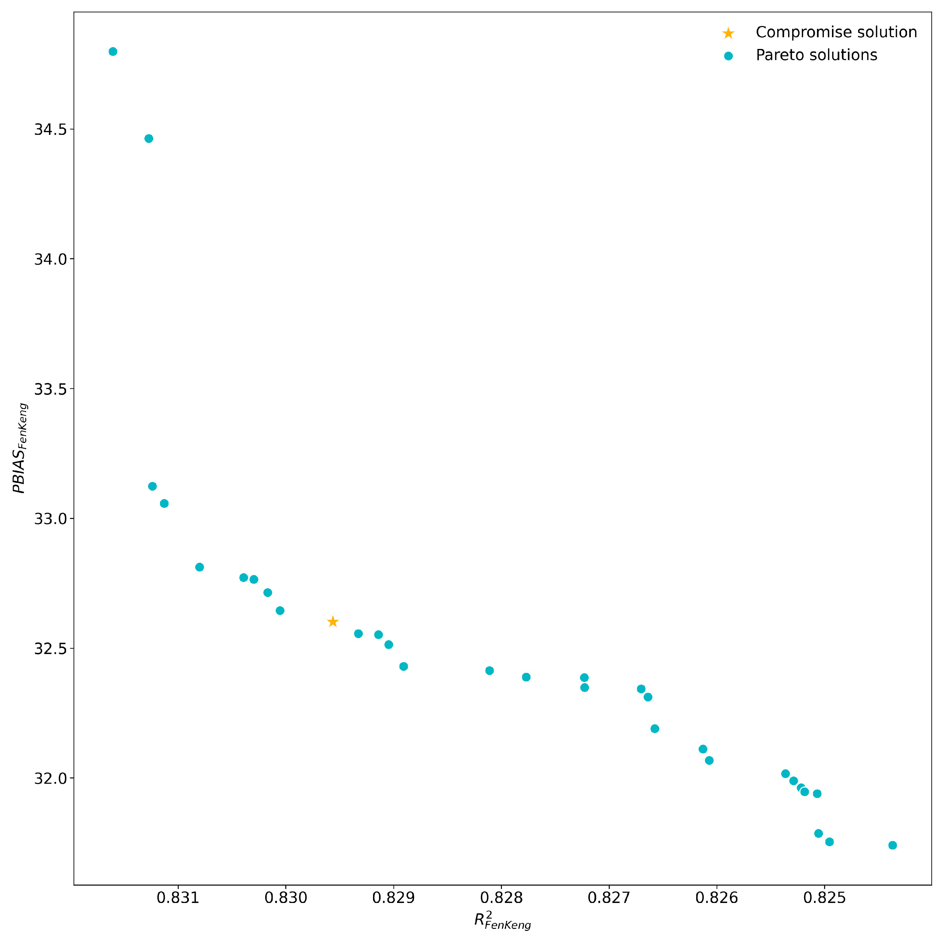
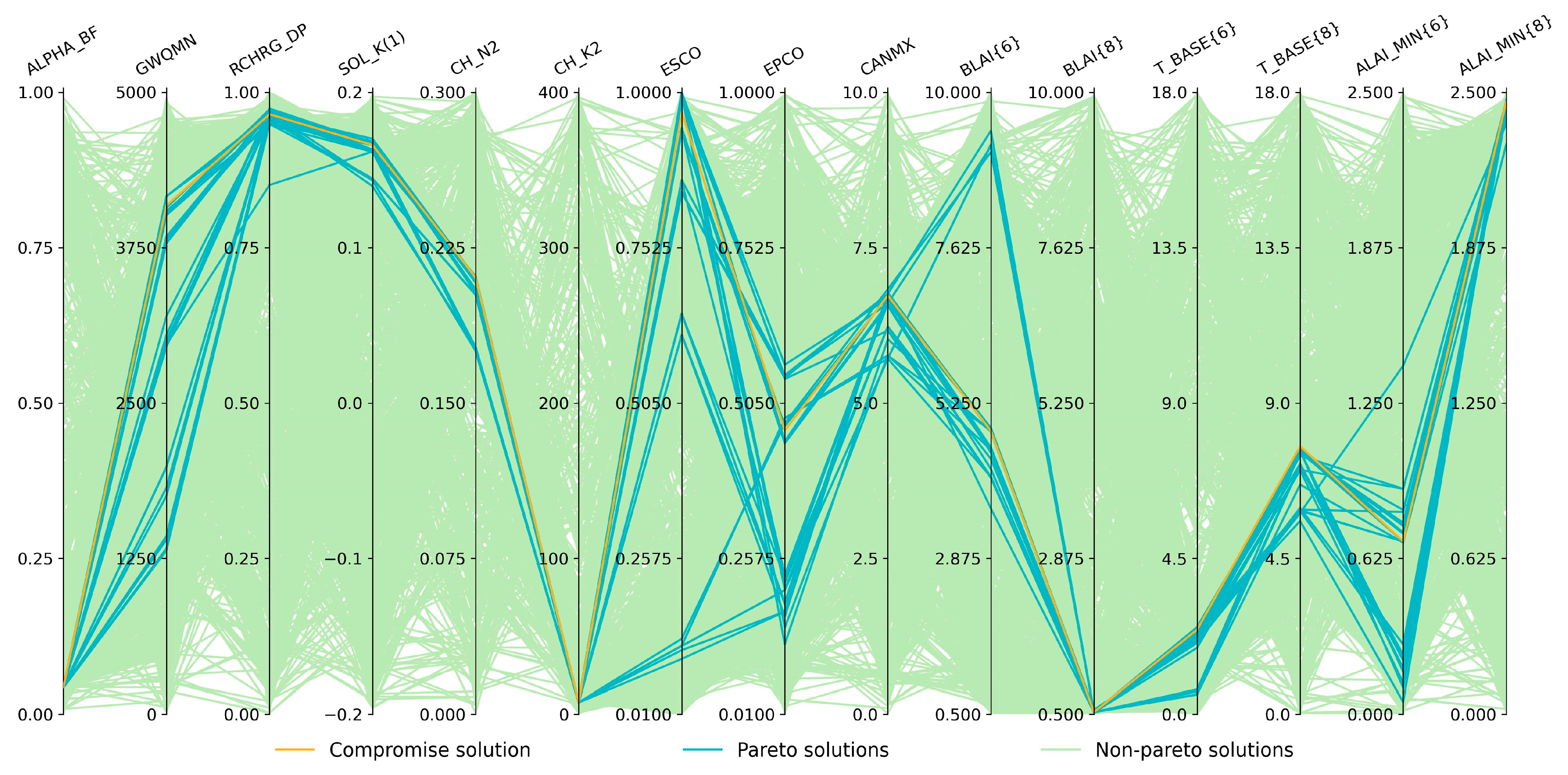
- Result Output/Result Plotting: The result output section outputs the Pareto and compromise solutions, parameter values during each generation, the number of non-dominated solutions during each generation, and the hypervolume during each generation to a text file. The result plotting section includes the hypervolume plot during each generation, the number of non-dominated solutions plot during each generation, the objective space distribution plot of Pareto and compromise solutions, the parallel coordinate plot of parameter values corresponding to non-Pareto, Pareto, and compromise solutions, time series plots of optimization variables (such as streamflow, leaf area index (LAI), ET, biomass), and flow duration curve plots;
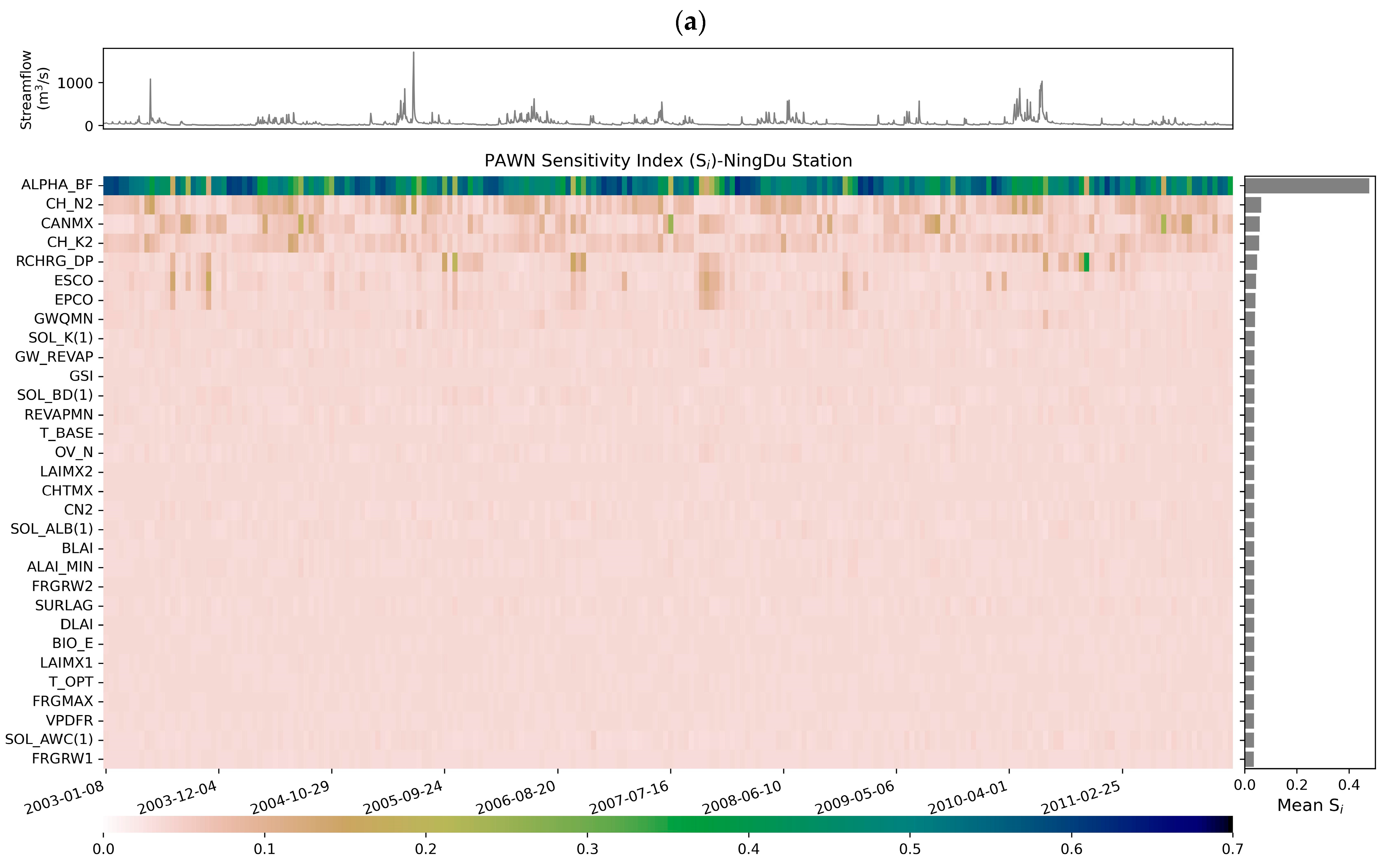
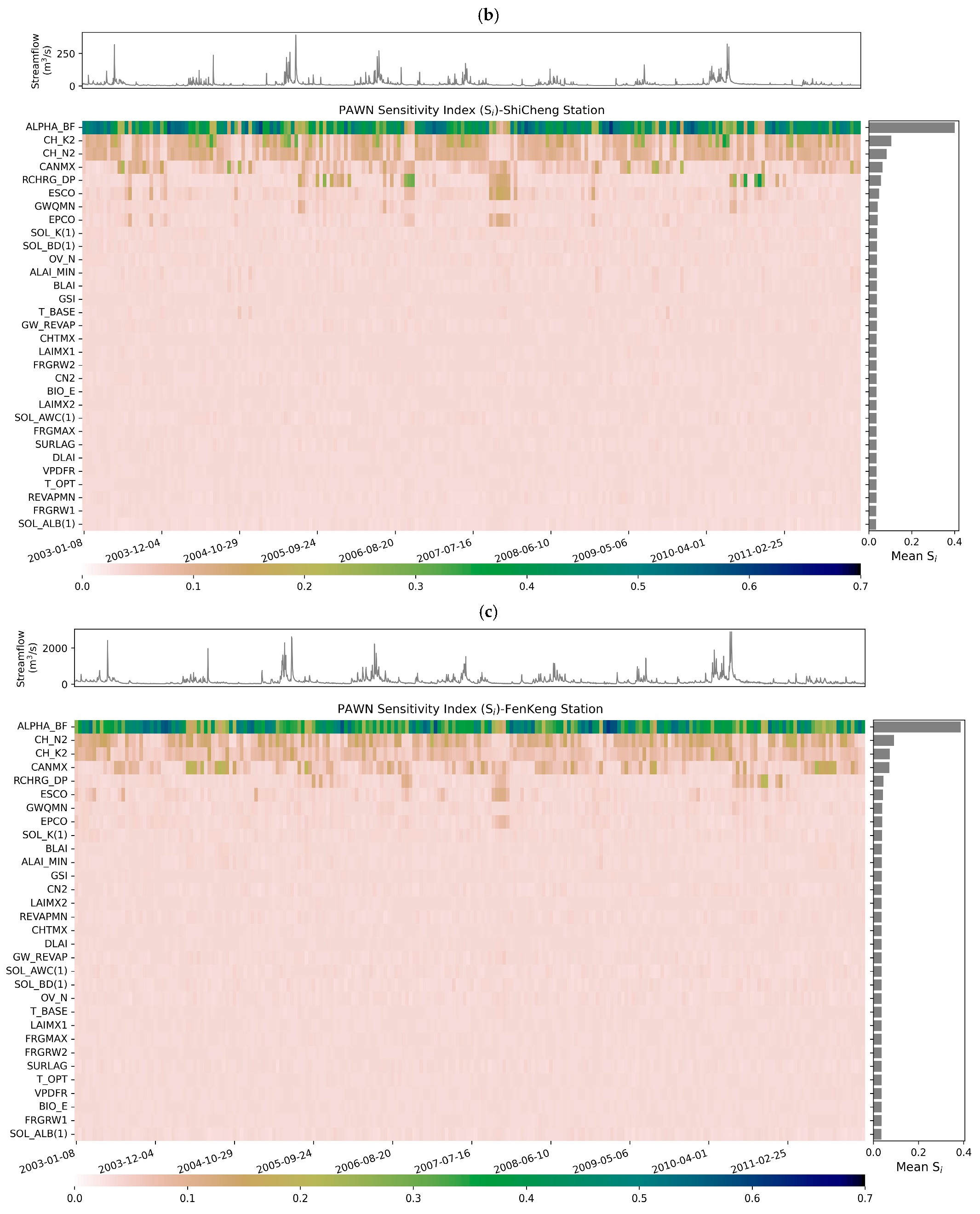
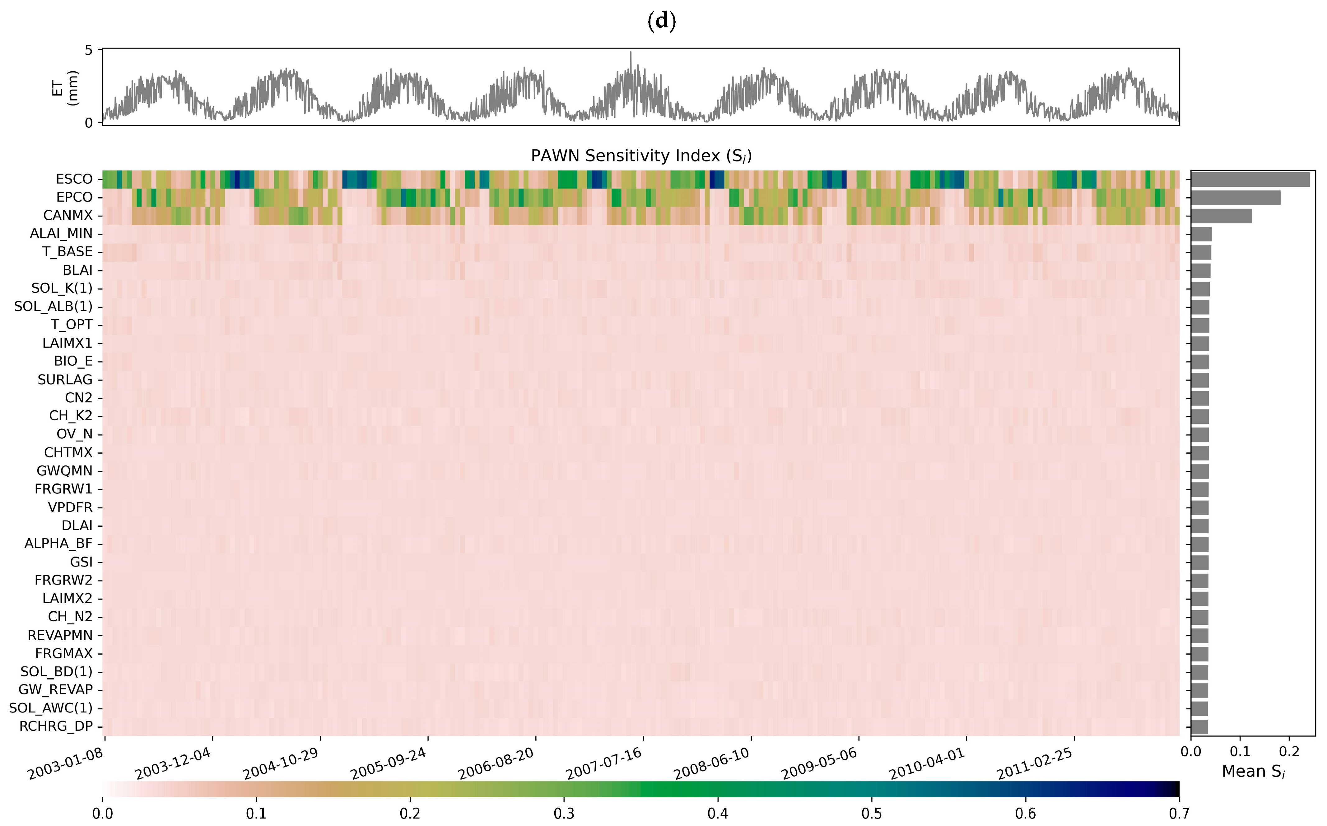
- Sensitivity Analysis: This includes Sobol’ [74] and PAWN [75] methods while time-varying sensitivity analysis (TVSA) is also supported for daily-scale long-time series data. The Sobol’ method is one of the most popular variance-based global sensitivity analysis methods [76,77]. It is a global analysis method based on variance decomposition, attributing the variance of model outputs to individual parameters and their interactions. For detailed information on using Sobol’s method to calculate hydrological model sensitivity, refer to [76,77]. One major limitation of variance-based sensitivity indices is that they require a large number of output samples to obtain accurate estimates; another major limitation is that they implicitly assume that output variance is a sensible measure of the output uncertainty, which might not always be the case [75]. To address these issues, a density-based GSA method, PAWN [75,78], has been proposed. PAWN uses the entire model output distribution, rather than just its variance, to quantify the relative influence of parameters on model outputs. By definition, the PAWN method is a moment-independent GSA method. It is very easy to implement, and the analysis of the robustness and convergence of PAWN sensitivity indices is computationally efficient.
- Reading Model Parameter File: Read the parameter names and corresponding ranges from the model parameter file (SWAT_Par.def). The definition of model parameters in this file is mainly according to the specifications in the SWAT-CUP software [18,52]. Parameters of the same type (determined by the parameter file suffix, e.g., .mgt, .gw, .sol, .rte, .hru, .bsn, .sub, and .plant.dat) are stored in a Python dictionary. The parameterization methods and value ranges of all parameters are also stored;
- Modifying Model Control File/Copy Model Project Files (in parallel): Based on user settings (such as simulation years, simulation start year, simulation output time interval, and warm-up period), modify the model control file (file.cio), then copy the model TxtInOut project folder to the parallel run directory according to the population size of the U-NSGA-III algorithm;
- Reading Observation Data (in parallel): Read the observation data, including the subbasin and HRU scale. For spatial distribution data, a watershed weighted average value is used, and the calculation formula is as follows, taking ET data as an example. For daily-scale spatial distribution data, the framework provides zonal statistics and outputs them to text files.where is the average ET for month (or day) j; is the total surface area of the watershed; is the surface area of subbasin (or HRU) i; is the ET for subbasin (or HRU) i and month (or day) j; and n is the number of subbasins (or HRUs);
- Modifying Model Parameters (in parallel): As with SWAT-CUP, it incorporates three parameterization methods (r for percentage change; v for replacement; and a for addition; see the SWAT-CUP manual for further details), which facilitates the alteration of diverse types of parameters, including those about vegetation, soil, management, groundwater, and so on. The initial parameterization values are derived from LHS, and subsequently from the optimized values of the previous generation;
- Executing the Model (in parallel): Call the SWAT.exe executable in each parallel run directory;
- Reading Model Simulation Data (in parallel): Read the data from the model output files (output.rch, output.sub, output.hru). Similar to step 3, a watershed weighted average value for spatial distribution data is established;
- Calculating Objective Functions (in parallel): Calculate the objective functions based on the observed and simulated data. The currently available objective functions include NSE [79], KGE [80], R2, PBIAS [81], and Root Mean Square Error (RMSE). They are calculated as the following:where and are the simulated and observed data; and are the means of simulated and observed data; is the linear regression coefficient between simulated and measured data; , , and are the means of simulated and measured data; and are the standard deviation of simulated and measured data; and is the number of observations. Here, PBIAS uses absolute values for calculation.
- (1)
- When performing a sensitivity analysis, the calculation of the objective function values in step 7 in the second module is passed directly to the sensitivity analysis part in the first module;
- (2)
- When multi-objective optimization is performed, initially, the number of parameters, the upper and lower bounds of each parameter, the number of objective functions, the number of constraints, the parameterized values for each generation, and the value of the objective functions for the current generation of the population computed in the last step in the second module are passed on to the third module. Subsequently, the optimization problem defined in the third module is passed on to the first module to perform the multi-objective optimization. When the model running reaches the maximum number of generations, the optimization result (approximate Pareto solutions) is subjected to a Multi-Criteria Decision Making (MCDM) process (selection of compromise solution from a set of Pareto solutions), followed by Convergence Analysis and Result Output/Result Plotting; otherwise, the optimized parameter values are passed to step 4 in the second module to continue the multi-objective optimization process.
3. Case Studies
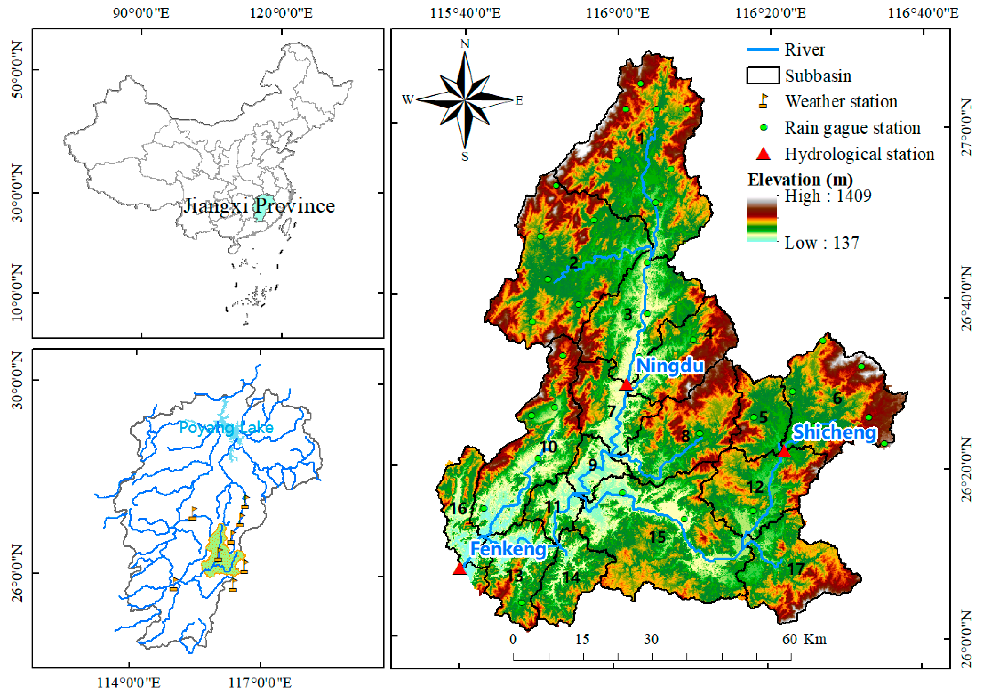
3.1. Study Area
3.2. Input Data and Model Setup

| Data Type | Spatial/Temporal Resolution | Source |
|---|---|---|
| Digital Elevation Model (DEM) | 30 m | ASTER GDEM (https://lpdaac.usgs.gov/products/astgtmv003/, accessed on 21 October 2024) |
| Land use | 30 m | ChinaCover2010 (Wu, et al. [86], http://www.geodata.cn, accessed on 21 October 2024) |
| Soil type | 30 m | 1:1,000,000 Soil Map of the China (https://www.resdc.cn/Default.aspx, accessed on 21 October 2024) |
| Soil properties | / | Basic soil property dataset of high-resolution China Soil Information Grids (2010–2018) (http://soil.geodata.cn, accessed on 21 October 2024) |
| Climate | Daily (2001–2011) | CMDC (China Meteorological Data Service Center) (http://data.cma.cn/, accessed on 21 October 2024) |
| Rainfall | Daily (2001–2011) | Annual Hydrological Report (Volume VI: Hydrological Data of Changjiang River Basin) |
| Streamflow | Daily (2001–2011) | Annual Hydrological Report (Volume VI: Hydrological Data of Changjiang River Basin) |
| ET | Daily (2001–2011)/500 m | PML-V2(China) (He, et al. [87]) |
3.3. Model Calibration
- (1)
- Multi-site calibration;
- (2)
- Multi-variable calibration;
- (3)
- Multi-objective functions calibration.
3.4. Efficiency Evaluation Metrics
3.5. Results
3.5.1. Sensitivity Analyses
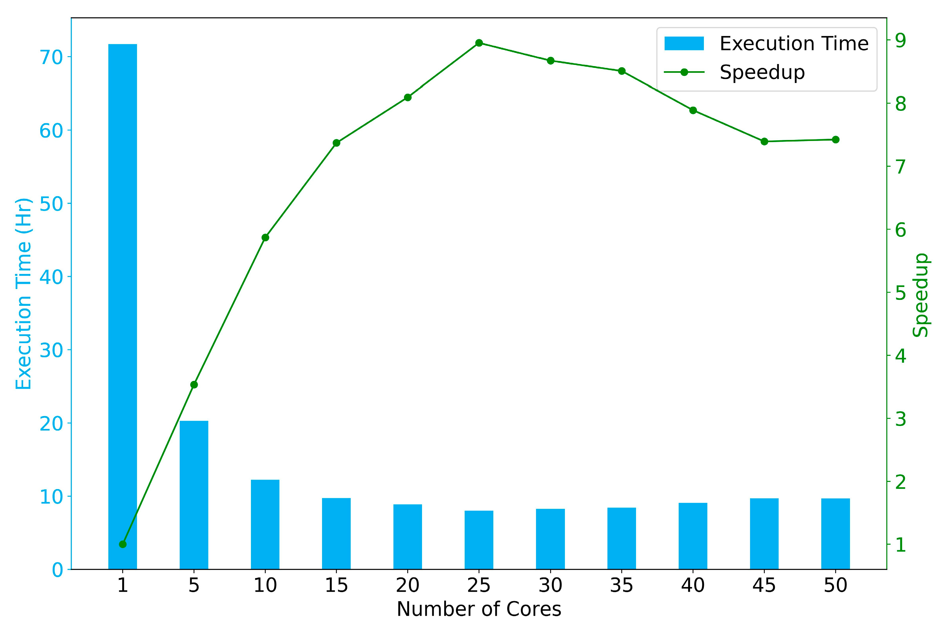
3.5.2. Efficiency Evaluation
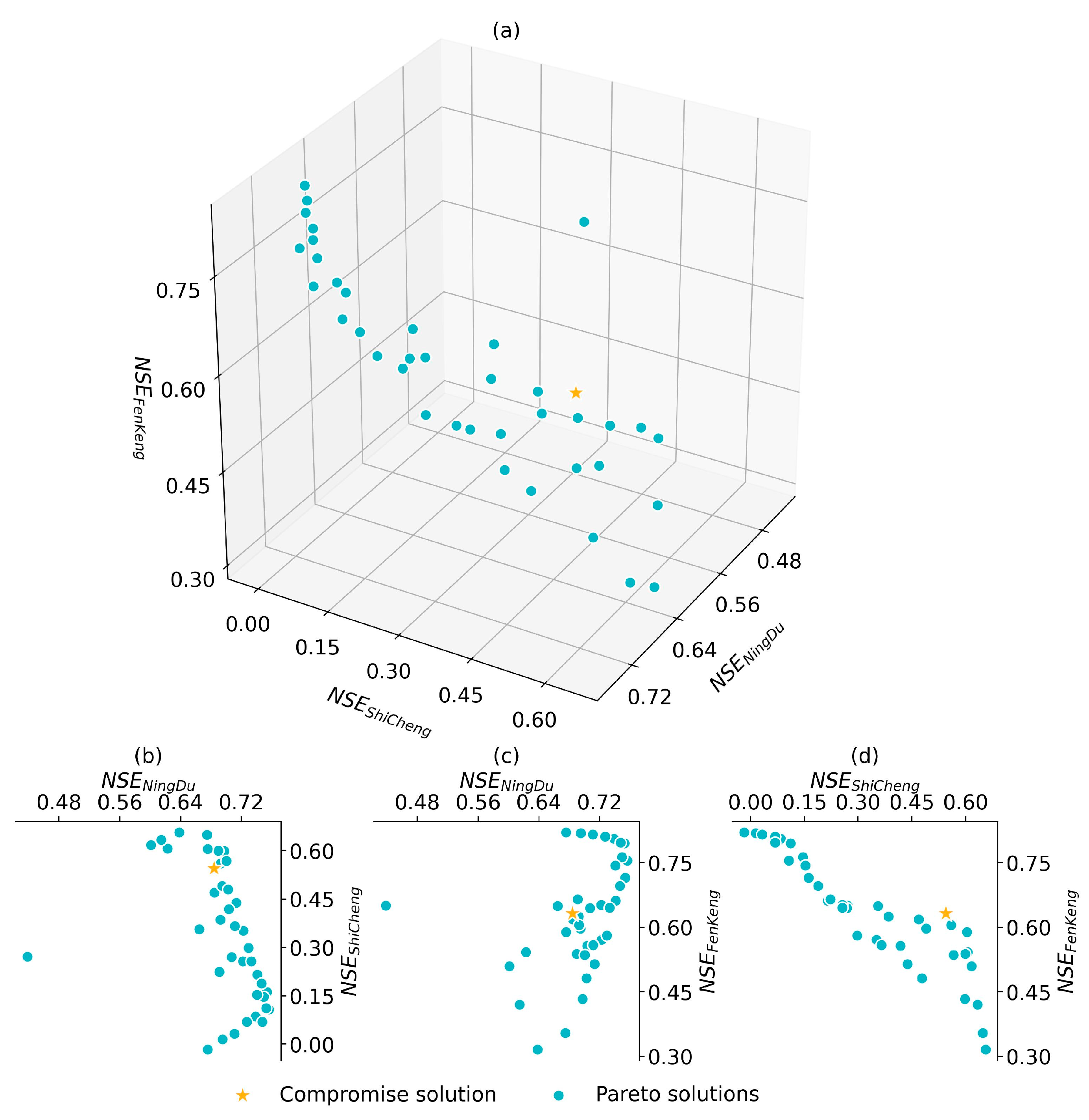
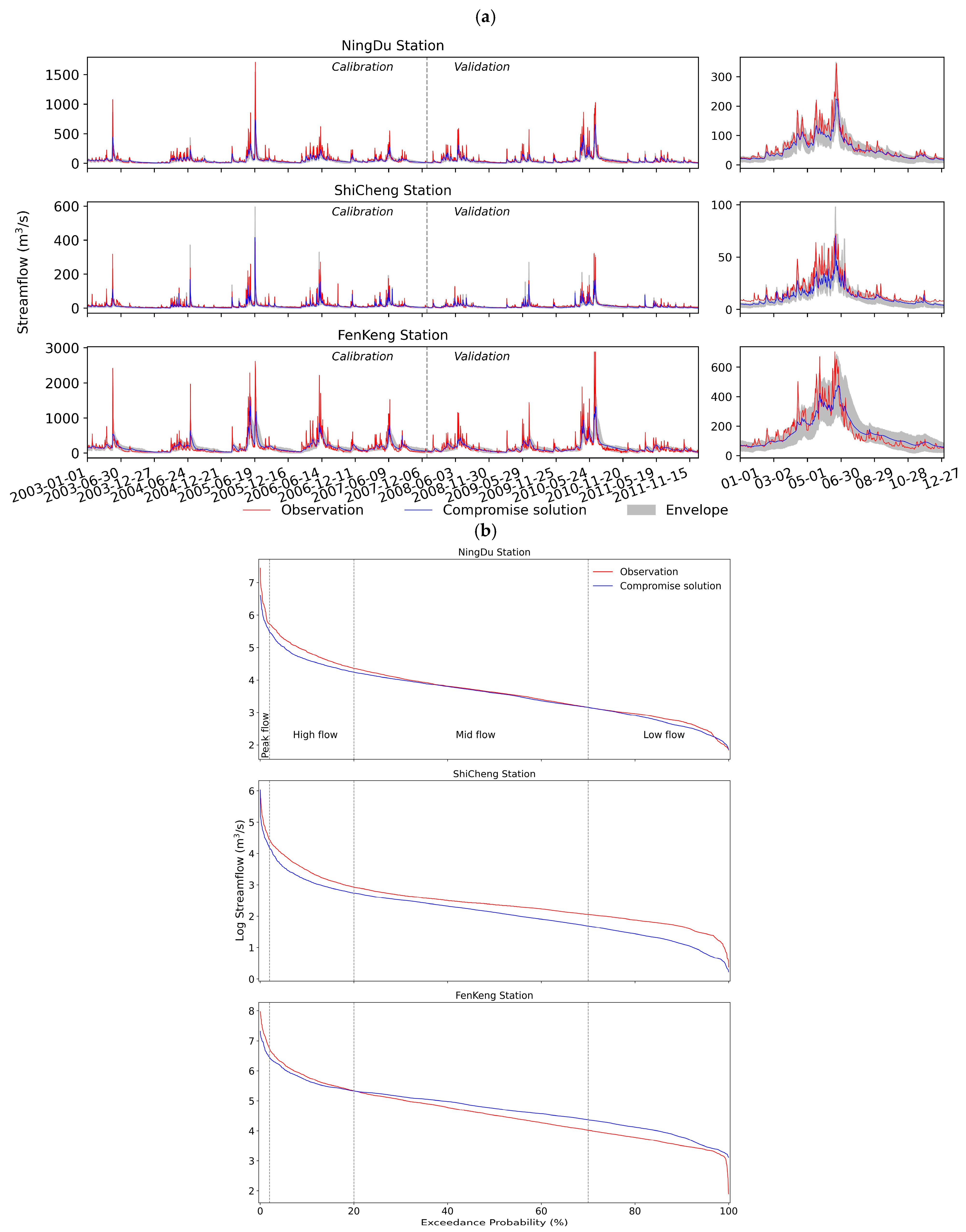
3.5.3. Example 1: Multi-Site Calibration
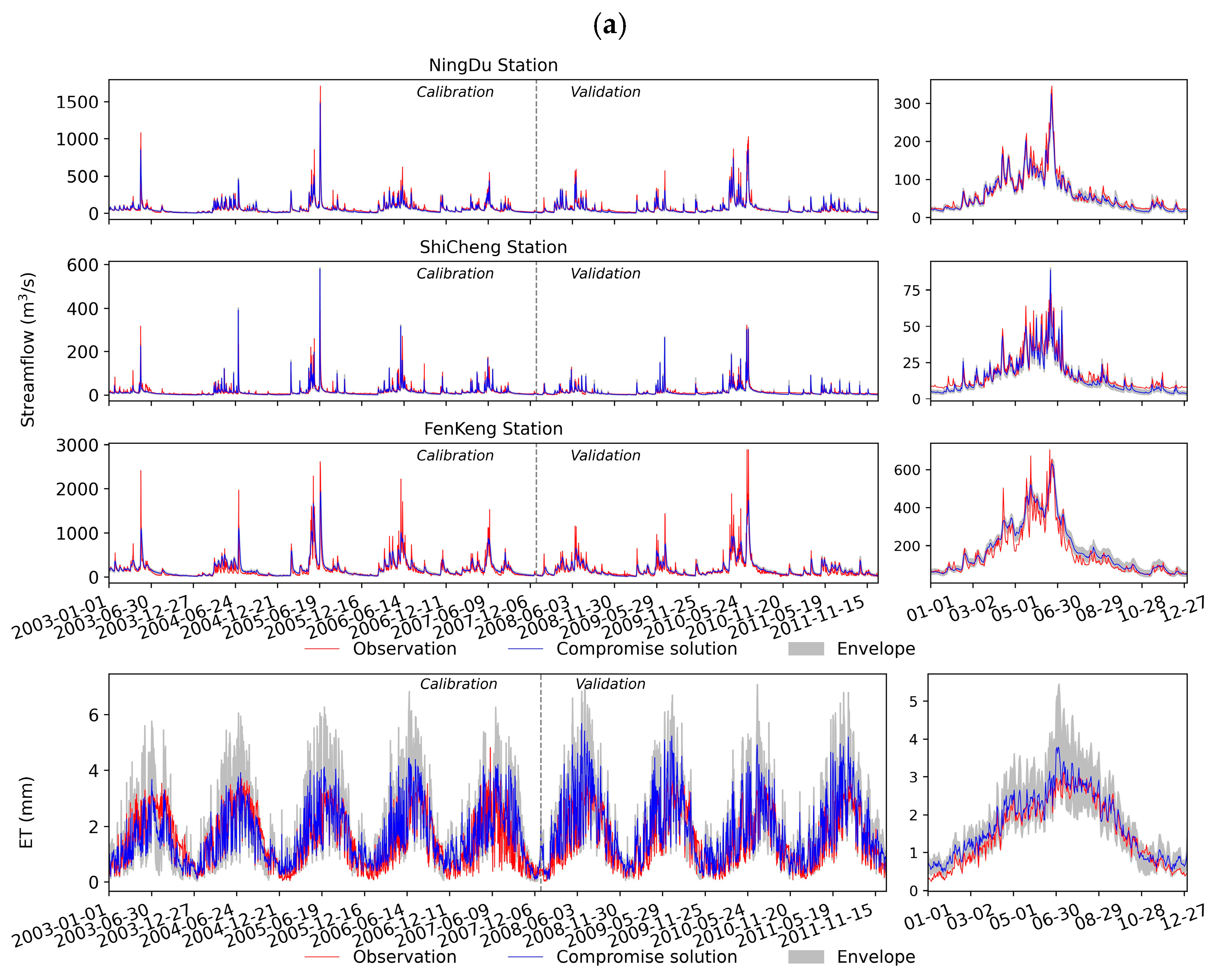
3.5.4. Example 2: Multi-Variable Calibration
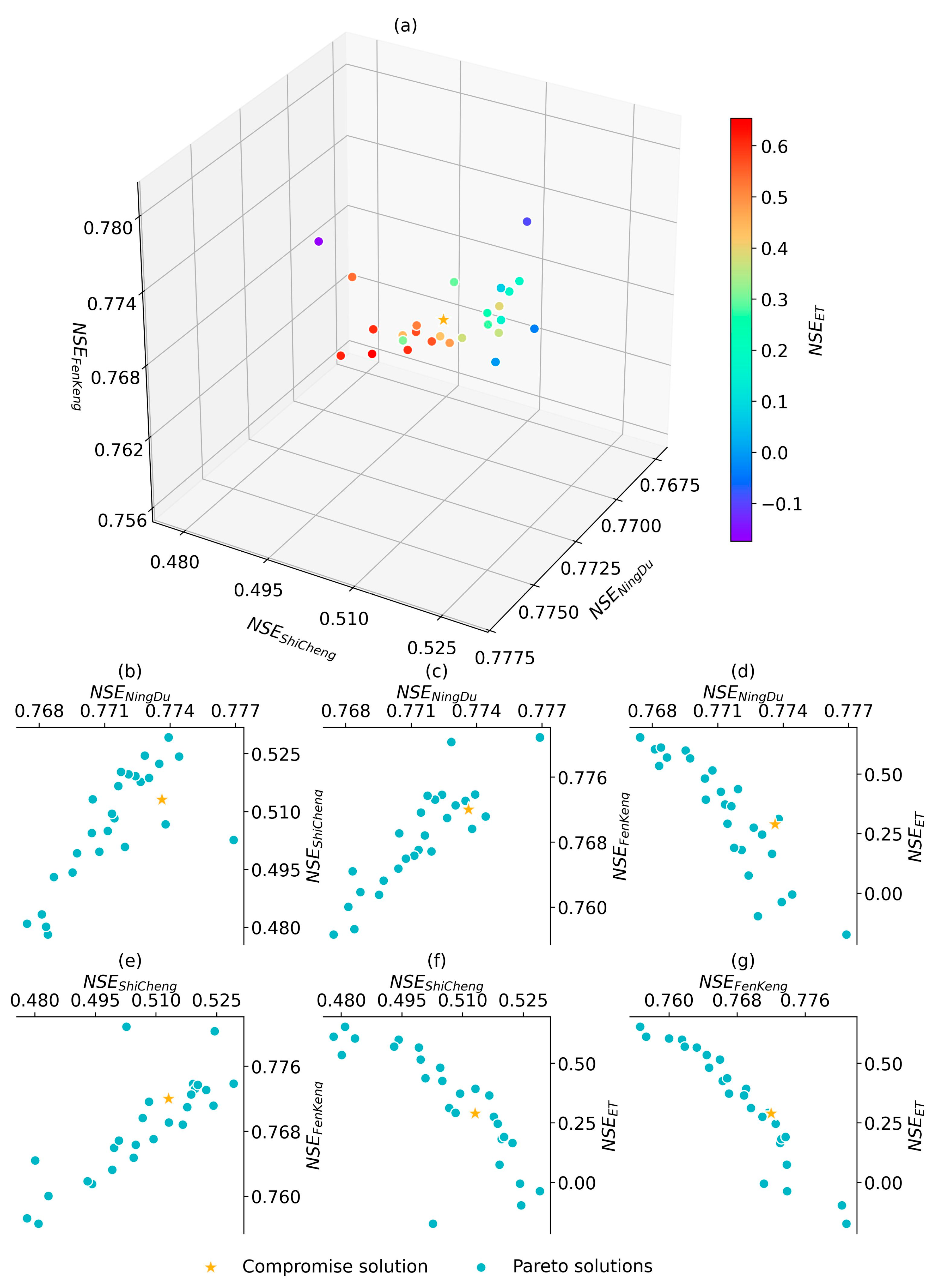
3.5.5. Example 3: Multi-Objective Functions Calibration
4. Discussion
4.1. Performance Analysis
4.2. Advantages, Limitations, and Future Directions
4.3. Prospects for Data-Driven Machine Learning Models (DMLs) and Process-Driven Hydrological Models (PHMs) in Hydrology
- (1)
- DMLs can handle various input variables flexibly, including non-traditional hydrological measurements;
- (2)
- DMLs can capture complex nonlinear relationships between input and output data;
- (3)
- In many hydrological applications, DMLs typically outperform physics-based and conceptual models in terms of predictive accuracy.
- (1)
- Despite significant successes across numerous fields, including hydrology, DMLs often face criticism for their lack of interpretability and physical consistency, referred to as “black box” models;
- (2)
- The performance of DMLs is heavily dependent on the quality and quantity of training data;
- (3)
- DMLs do not fundamentally understand the underlying physical mechanisms, limiting their ability to explain causal relationships between hydrological variables within processes. Additionally, they lack mass balance checks, making it impossible to ascertain how much water is converted from precipitation and how much remains within the watershed;
- (4)
- DMLs may struggle to capture the effects of non-stationarity, as they assume that the training and testing data distributions are the same;
- (5)
- Deep learning models typically require substantial computational resources, including high-performance computing (HPC) systems and graphics processing units (GPUs) for training and inference, with computational demands increasing as hydrological datasets become larger and more complex.
- (1)
- PHMs are based on the physical laws governing hydrological processes, thus providing a solid theoretical foundation and interpretability; the parameters in PHMs have clear physical meanings, facilitating calibration and adjustment based on actual hydrological processes;
- (2)
- PHMs generally exhibit robust predictions across different conditions and regions once parameters have been appropriately calibrated;
- (3)
- PHMs can be applied to various watersheds and climatic conditions, offering good generalizability.
- (1)
- PHMs often face constraints related to parameterization adequacy, data quality and uncertainty, computational limitations, complexity, and availability;
- (2)
- PHMs may struggle when simulating complex nonlinear hydrological processes, potentially failing to adequately capture spatial dependencies across different temporal and spatial scales;
- (3)
- PHMs might introduce higher uncertainties due to differences in datasets, model parameters, and model structures.
5. Conclusions
Supplementary Materials
Author Contributions
Funding
Data Availability Statement
Acknowledgments
Conflicts of Interest
References
- Wagener, T.; Boyle, D.P.; Lees, M.J.; Wheater, H.S.; Gupta, H.V.; Sorooshian, S. A framework for development and application of hydrological models. Hydrol. Earth Syst. Sci. 2001, 5, 13–26. [Google Scholar] [CrossRef]
- Clark, M.P.; Fan, Y.; Lawrence, D.M.; Adam, J.C.; Bolster, D.; Gochis, D.J.; Hooper, R.P.; Kumar, M.; Leung, L.R.; Mackay, D.S.; et al. Improving the representation of hydrologic processes in Earth System Models. Water Resour. Res. 2015, 51, 5929–5956. [Google Scholar] [CrossRef]
- Moges, E.; Demissie, Y.; Larsen, L.; Yassin, F. Review: Sources of Hydrological Model Uncertainties and Advances in Their Analysis. Water 2021, 13, 28. [Google Scholar] [CrossRef]
- Gassman, P.W.; Reyes, M.R.; Green, C.H.; Arnold, J.G. The soil and water assessment tool: Historical development, applications, and future research directions. Trans. ASABE 2007, 50, 1211–1250. [Google Scholar] [CrossRef]
- Keller, A.A.; Garner, K.; Rao, N.; Knipping, E.; Thomas, J. Hydrological models for climate-based assessments at the watershed scale: A critical review of existing hydrologic and water quality models. Sci. Total Environ. 2023, 867, 161209. [Google Scholar] [CrossRef]
- Beven, K. How far can we go in distributed hydrological modelling? Hydrol. Earth Syst. Sci. 2001, 5, 1–12. [Google Scholar] [CrossRef]
- Fatichi, S.; Vivoni, E.R.; Ogden, F.L.; Ivanov, V.Y.; Mirus, B.; Gochis, D.; Downer, C.W.; Camporese, M.; Davison, J.H.; Ebel, B.; et al. An overview of current applications, challenges, and future trends in distributed process-based models in hydrology. J. Hydrol. 2016, 537, 45–60. [Google Scholar] [CrossRef]
- Beven, K.J. Rainfall-Runoff Modelling: The Primer, 2nd ed.; John Wiley & Sons: Hoboken, NJ, USA, 2012. [Google Scholar]
- Gao, H.; Birkel, C.; Hrachowitz, M.; Tetzlaff, D.; Soulsby, C.; Savenije, H.H.G. A simple topography-driven and calibration-free runoff generation module. Hydrol. Earth Syst. Sci. 2019, 23, 787–809. [Google Scholar] [CrossRef]
- Babović, V.; Wu, Z.; Larsen, L.C. Calibrating hydrodynamic models by means of simulated evolution. In Proceedings of the First International Conference on Hydroinformatics (Hydroinformatics ’94), Rotterdam, The Netherlands, 19–23 September 1994; pp. 193–200. [Google Scholar]
- Savic, D.A.; Walters, G.A. Genetic Algorithms for Least-Cost Design of Water Distribution Networks. J. Water Resour. Plan. Manag. 1997, 123, 67–77. [Google Scholar] [CrossRef]
- Khu, S.T.; Madsen, H. Multiobjective calibration with Pareto preference ordering: An application to rainfall-runoff model calibration. Water Resour. Res. 2005, 41, W03004. [Google Scholar] [CrossRef]
- Hernandez-Suarez, J.S.; Nejadhashemi, A.P.; Deb, K. A novel multi-objective model calibration method for ecohydrological applications. Environ. Model. Softw. 2021, 144, 105161. [Google Scholar] [CrossRef]
- Ercan, M.B.; Goodall, J.L. Design and implementation of a general software library for using NSGA-II with SWAT for multi-objective model calibration. Environ. Model. Softw. 2016, 84, 112–120. [Google Scholar] [CrossRef]
- Beven, K.; Freer, J. Equifinality, data assimilation, and uncertainty estimation in mechanistic modelling of complex environmental systems using the GLUE methodology. J. Hydrol. 2001, 249, 11–29. [Google Scholar] [CrossRef]
- Arnold, J.G.; Srinivasan, R.; Muttiah, R.S.; Williams, J.R. Large area hydrologic modeling and assessment. Part I: Model development. JAWRA J. Am. Water Resour. Assoc. 1998, 34, 73–89. [Google Scholar] [CrossRef]
- Douglas-Mankin, K.R.; Srinivasan, R.; Arnold, J.G. Soil and Water Assessment Tool (SWAT) Model: Current Developments and Applications. Trans. ASABE 2010, 53, 1423–1431. [Google Scholar] [CrossRef]
- Abbaspour, K.C.; Vejdani, M.; Haghighat, S.; Yang, J. SWAT-CUP calibration and uncertainty programs for SWAT. In Proceedings of the MODSIM 2007 International Congress on Modelling and Simulation, Modelling and Simulation Society of Australia and New Zealand, Christchurch, New Zealand, 5 December 2007; pp. 1596–1602. [Google Scholar]
- Krishnan, N.; Raj, C.; Chaubey, I.; Sudheer, K.P. Parameter estimation of SWAT and quantification of consequent confidence bands of model simulations. Environ. Earth Sci. 2018, 77, 470. [Google Scholar] [CrossRef]
- Ercan, M.B.; Goodall, J.L.; Castronova, A.M.; Humphrey, M.; Beekwilder, N. Calibration of SWAT models using the cloud. Environ. Model. Softw. 2014, 62, 188–196. [Google Scholar] [CrossRef]
- Zhang, X.; Srinivasan, R.; Zhao, K.; Liew, M.V. Evaluation of global optimization algorithms for parameter calibration of a computationally intensive hydrologic model. Hydrol. Process. 2009, 23, 430–441. [Google Scholar] [CrossRef]
- Duan, Q.; Sorooshian, S.; Gupta, V. Effective and efficient global optimization for conceptual rainfall-runoff models. Water Resour. Res. 1992, 28, 1015–1031. [Google Scholar] [CrossRef]
- Kavetski, D.; Qin, Y.; Kuczera, G. The Fast and the Robust: Trade-Offs Between Optimization Robustness and Cost in the Calibration of Environmental Models. Water Resour. Res. 2018, 54, 9432–9455. [Google Scholar] [CrossRef]
- Vrugt, J.A.; Gupta, H.V.; Bouten, W.; Sorooshian, S. A Shuffled Complex Evolution Metropolis algorithm for optimization and uncertainty assessment of hydrologic model parameters. Water Resour. Res. 2003, 39, 1201. [Google Scholar] [CrossRef]
- Tolson, B.A.; Shoemaker, C.A. Dynamically dimensioned search algorithm for computationally efficient watershed model calibration. Water Resour. Res. 2007, 43, W01413. [Google Scholar] [CrossRef]
- Efstratiadis, A.; Koutsoyiannis, D. One decade of multi-objective calibration approaches in hydrological modelling: A review. Hydrol. Sci. J. 2010, 55, 58–78. [Google Scholar] [CrossRef]
- Gupta, H.V.; Sorooshian, S.; Yapo, P.O. Toward improved calibration of hydrologic models: Multiple and noncommensurable measures of information. Water Resour. Res. 1998, 34, 751–763. [Google Scholar] [CrossRef]
- Yapo, P.O.; Gupta, H.V.; Sorooshian, S. Multi-objective global optimization for hydrologic models. J. Hydrol. 1998, 204, 83–97. [Google Scholar] [CrossRef]
- Bekele, E.G.; Nicklow, J.W. Multi-objective automatic calibration of SWAT using NSGA-II. J. Hydrol. 2007, 341, 165–176. [Google Scholar] [CrossRef]
- Zhang, X.; Srinivasan, R.; Van Liew, M. Multi-Site Calibration of the SWAT Model for Hydrologic Modeling. Trans. ASABE 2008, 51, 2039–2049. [Google Scholar] [CrossRef]
- Rajib, M.A.; Merwade, V.; Yu, Z.Q. Multi-objective calibration of a hydrologic model using spatially distributed remotely sensed/in-situ soil moisture. J. Hydrol. 2016, 536, 192–207. [Google Scholar] [CrossRef]
- Herman, M.R.; Nejadhashemi, A.P.; Abouali, M.; Hernandez-Suarez, J.S.; Daneshvar, F.; Zhang, Z.; Anderson, M.C.; Sadeghi, A.M.; Hain, C.R.; Sharifi, A. Evaluating the role of evapotranspiration remote sensing data in improving hydrological modeling predictability. J. Hydrol. 2018, 556, 39–49. [Google Scholar] [CrossRef]
- Chilkoti, V.; Bolisetti, T.; Balachandar, R. Multi-objective autocalibration of SWAT model for improved low flow performance for a small snowfed catchment. Hydrol. Sci. J.-J. Des Sci. Hydrol. 2018, 63, 1482–1501. [Google Scholar] [CrossRef]
- Herman, M.R.; Hernandez-Suarez, J.S.; Nejadhashemi, A.P.; Kropp, I.; Sadeghi, A.M. Evaluation of Multi- and Many-Objective Optimization Techniques to Improve the Performance of a Hydrologic Model Using Evapotranspiration Remote-Sensing Data. J. Hydrol. Eng. 2020, 25, 04020006. [Google Scholar] [CrossRef]
- Mohammadi Igder, O.; Alizadeh, H.; Mojaradi, B.; Bayat, M. Multivariate assimilation of satellite-based leaf area index and ground-based river streamflow for hydrological modelling of irrigated watersheds using SWAT+. J. Hydrol. 2022, 610, 128012. [Google Scholar] [CrossRef]
- Sheffield, J.; Wood, E.F.; Pan, M.; Beck, H.; Coccia, G.; Serrat-Capdevila, A.; Verbist, K. Satellite Remote Sensing for Water Resources Management: Potential for Supporting Sustainable Development in Data-Poor Regions. Water Resour. Res. 2018, 54, 9724–9758. [Google Scholar] [CrossRef]
- Jiang, D.; Wang, K. The Role of Satellite-Based Remote Sensing in Improving Simulated Streamflow: A Review. Water 2019, 11, 1615. [Google Scholar] [CrossRef]
- Dembélé, M.; Ceperley, N.; Zwart, S.J.; Salvadore, E.; Mariethoz, G.; Schaefli, B. Potential of satellite and reanalysis evaporation datasets for hydrological modelling under various model calibration strategies. Adv. Water Resour. 2020, 143, 103667. [Google Scholar] [CrossRef]
- Rajib, A.; Evenson, G.R.; Golden, H.E.; Lane, C.R. Hydrologic model predictability improves with spatially explicit calibration using remotely sensed evapotranspiration and biophysical parameters. J. Hydrol. 2018, 567, 668–683. [Google Scholar] [CrossRef]
- Deb, K. Multi-objective Optimisation Using Evolutionary Algorithms: An Introduction. In Multi-Objective Evolutionary Optimisation for Product Design and Manufacturing; Deb, K., Ed.; Springer: London, UK, 2011; pp. 3–34. [Google Scholar]
- Reed, P.M.; Hadka, D.; Herman, J.D.; Kasprzyk, J.R.; Kollat, J.B. Evolutionary multiobjective optimization in water resources: The past, present, and future. Adv. Water Resour. 2013, 51, 438–456. [Google Scholar] [CrossRef]
- Zhang, X.; Beeson, P.; Link, R.; Manowitz, D.; Izaurralde, R.C.; Sadeghi, A.; Thomson, A.M.; Sahajpal, R.; Srinivasan, R.; Arnold, J.G. Efficient multi-objective calibration of a computationally intensive hydrologic model with parallel computing software in Python. Environ. Model. Softw. 2013, 46, 208–218. [Google Scholar] [CrossRef]
- Vrugt, J.A.; Robinson, B.A. Improved evolutionary optimization from genetically adaptive multimethod search. Proc. Natl. Acad. Sci. USA 2007, 104, 708–711. [Google Scholar] [CrossRef]
- Besalatpour, A.A.; Pourreza-Bilondi, M.; Aghakhani Afshar, A. Parallelization of AMALGAM algorithm for a multi-objective optimization of a hydrological model. Appl. Water Sci. 2023, 13, 241. [Google Scholar] [CrossRef]
- Zhang, X.; Srinivasan, R.; Liew, M.V. On the use of multi-algorithm, genetically adaptive multi-objective method for multi-site calibration of the SWAT model. Hydrol. Process. 2010, 24, 955–969. [Google Scholar] [CrossRef]
- Zamani, M.; Shrestha, N.K.; Akhtar, T.; Boston, T.; Daggupati, P. Advancing model calibration and uncertainty analysis of SWAT models using cloud computing infrastructure: LCC-SWAT. J. Hydroinformatics 2020, 23, 1–15. [Google Scholar] [CrossRef]
- Confesor, R.B.; Whittaker, G.W. Automatic calibration of hydrologic models with multi-objective evolutionary algorithm and Pareto optimization. J. Am. Water Resour. Assoc. 2007, 43, 981–989. [Google Scholar] [CrossRef]
- Her, Y.; Cibin, R.; Chaubey, I. Application of Parallel Computing Methods for Improving Efficiency of Optimization in Hydrologic and Water Quality Modeling. Appl. Eng. Agric. 2015, 31, 455–468. [Google Scholar] [CrossRef]
- Kayastha, N.; Lu, S.; Betrie, G.; Zakayo, Z.; van Griensven, A.; Solomatine, D. Dynamic linking of the watershed model SWAT to the multi-objective optimization tool NSGAX. In Proceedings of the Watermatex, 8th IWA Symposium on Systems Analysis and Integrated Assessment, IWA, San Sebastian, Spain, 20–22 June 2011; pp. 10–15. [Google Scholar]
- Zhang, X.; Izaurralde, R.C.; Zong, Z.; Zhao, K.; Thomson, A.M. Evaluating the Efficiency of a Multi-core Aware Multi-objective Optimization Tool for Calibrating the SWAT Model. Trans. ASABE 2012, 55, 1723–1731. [Google Scholar] [CrossRef]
- Rouholahnejad, E.; Abbaspour, K.C.; Vejdani, M.; Srinivasan, R.; Schulin, R.; Lehmann, A. A parallelization framework for calibration of hydrological models. Environ. Model. Softw. 2012, 31, 28–36. [Google Scholar] [CrossRef]
- Abbaspour, K.C. SWAT-CUP: SWAT Calibration and Uncertainty Programs—A User Manual; Eawag: Dübendorf, Switzerland, 2015; pp. 16–70. [Google Scholar]
- Zhang, X.; Srinivasan, R.; Hao, F. Predicting Hydrologic Response to Climate Change in the Luohe River Basin Using the SWAT Model. Trans. ASABE 2007, 50, 901–910. [Google Scholar] [CrossRef]
- Nijzink, R.C.; Almeida, S.; Pechlivanidis, I.G.; Capell, R.; Gustafssons, D.; Arheimer, B.; Parajka, J.; Freer, J.; Han, D.; Wagener, T.; et al. Constraining Conceptual Hydrological Models With Multiple Information Sources. Water Resour. Res. 2018, 54, 8332–8362. [Google Scholar] [CrossRef]
- Pool, S.; Fowler, K.; Peel, M. Benefit of Multivariate Model Calibration for Different Climatic Regions. Water Resour. Res. 2024, 60, e2023WR036364. [Google Scholar] [CrossRef]
- Mahmood, R.; Jia, S. A Comprehensive Approach to Develop a Hydrological Model for the Simulation of All the Important Hydrological Components: The Case of the Three-River Headwater Region, China. Water 2022, 14, 2778. [Google Scholar] [CrossRef]
- Ali, M.H.; Popescu, I.; Jonoski, A.; Solomatine, D.P. Remote Sensed and/or Global Datasets for Distributed Hydrological Modelling: A Review. Remote Sens. 2023, 15, 1642. [Google Scholar] [CrossRef]
- Deb, K.; Jain, H. An Evolutionary Many-Objective Optimization Algorithm Using Reference-Point-Based Nondominated Sorting Approach, Part I: Solving Problems With Box Constraints. IEEE Trans. Evol. Comput. 2014, 18, 577–601. [Google Scholar] [CrossRef]
- Köppen, M.; Yoshida, K. Substitute Distance Assignments in NSGA-II for Handling Many-objective Optimization Problems. In Proceedings of the Evolutionary Multi-Criterion Optimization; Springer: Berlin/Heidelberg, Germany, 2007; pp. 727–741. [Google Scholar]
- Seada, H.; Deb, K. A Unified Evolutionary Optimization Procedure for Single, Multiple, and Many Objectives. IEEE Trans. Evol. Comput. 2016, 20, 358–369. [Google Scholar] [CrossRef]
- Neitsch, S.L.; Arnold, J.G.; Kiniry, J.R.; Williams, J.R. Soil and Water Assessment Tool Theoretical Documentation Version 2009; Texas Water Resources Institute: College Station, TX, USA, 2011. [Google Scholar]
- Deb, K.; Pratap, A.; Agarwal, S.; Meyarivan, T. A fast and elitist multiobjective genetic algorithm: NSGA-II. IEEE Trans. Evol. Comput. 2002, 6, 182–197. [Google Scholar] [CrossRef]
- Lu, S.; Kayastha, N.; Thodsen, H.; van Griensven, A.; Andersen, H.E. Multiobjective Calibration for Comparing Channel Sediment Routing Models in the Soil and Water Assessment Tool. J. Environ. Qual. 2014, 43, 110–120. [Google Scholar] [CrossRef]
- Maringanti, C.; Chaubey, I.; Popp, J. Development of a multiobjective optimization tool for the selection and placement of best management practices for nonpoint source pollution control. Water Resour. Res. 2009, 45, W06406. [Google Scholar] [CrossRef]
- Jain, H.; Deb, K. An Evolutionary Many-Objective Optimization Algorithm Using Reference-Point Based Nondominated Sorting Approach, Part II: Handling Constraints and Extending to an Adaptive Approach. IEEE Trans. Evol. Comput. 2014, 18, 602–622. [Google Scholar] [CrossRef]
- Hernandez-Suarez, J.S.; Nejadhashemi, A.P. Probabilistic Predictions of Ecologically Relevant Hydrologic Indices Using a Hydrological Model. Water Resour. Res. 2022, 58, e2021WR031104. [Google Scholar] [CrossRef]
- Blank, J.; Deb, K.; Dhebar, Y.; Bandaru, S.; Seada, H. Generating Well-Spaced Points on a Unit Simplex for Evolutionary Many-Objective Optimization. IEEE Trans. Evol. Comput. 2021, 25, 48–60. [Google Scholar] [CrossRef]
- McKay, M.D.; Beckman, R.J.; Conover, W.J. A Comparison of Three Methods for Selecting Values of Input Variables in the Analysis of Output From a Computer Code. Technometrics 2000, 42, 55–61. [Google Scholar] [CrossRef]
- Blank, J.; Deb, K. Pymoo: Multi-Objective Optimization in Python. IEEE Access 2020, 8, 89497–89509. [Google Scholar] [CrossRef]
- Zeleny, M. Multiple Criteria Decision Making (MCDM): From Paradigm Lost to Paradigm Regained? J. Multi-Criteria Decis. Anal. 2011, 18, 77–89. [Google Scholar] [CrossRef]
- Deb, K. Multi-Objective Optimization Using Evolutionary Algorithms; John Wiley & Sons: Hoboken, NJ, USA, 2001; Volume 16. [Google Scholar]
- Zitzler, E.; Thiele, L. Multiobjective evolutionary algorithms: A comparative case study and the strength Pareto approach. IEEE Trans. Evol. Comput. 1999, 3, 257–271. [Google Scholar] [CrossRef]
- Singh, H.K. Understanding Hypervolume Behavior Theoretically for Benchmarking in Evolutionary Multi/Many-Objective Optimization. IEEE Trans. Evol. Comput. 2020, 24, 603–610. [Google Scholar] [CrossRef]
- Sobol’, I.y.M. On sensitivity estimation for nonlinear mathematical models. Mat. Model. 1990, 2, 112–118. [Google Scholar]
- Pianosi, F.; Wagener, T. A simple and efficient method for global sensitivity analysis based on cumulative distribution functions. Environ. Model. Softw. 2015, 67, 1–11. [Google Scholar] [CrossRef]
- Nossent, J.; Elsen, P.; Bauwens, W. Sobol’ sensitivity analysis of a complex environmental model. Environ. Model. Softw. 2011, 26, 1515–1525. [Google Scholar] [CrossRef]
- Zhang, C.; Chu, J.G.; Fu, G.T. Sobol’s sensitivity analysis for a distributed hydrological model of Yichun River Basin, China. J. Hydrol. 2013, 480, 58–68. [Google Scholar] [CrossRef]
- Pianosi, F.; Wagener, T. Distribution-based sensitivity analysis from a generic input-output sample. Environ. Model. Softw. 2018, 108, 197–207. [Google Scholar] [CrossRef]
- Nash, J.E.; Sutcliffe, J.V. River flow forecasting through conceptual models part I—A discussion of principles. J. Hydrol. 1970, 10, 282–290. [Google Scholar] [CrossRef]
- Gupta, H.V.; Kling, H.; Yilmaz, K.K.; Martinez, G.F. Decomposition of the mean squared error and NSE performance criteria: Implications for improving hydrological modelling. J. Hydrol. 2009, 377, 80–91. [Google Scholar] [CrossRef]
- Gupta, H.; Sorooshian, S.; Yapo, P. Status of Automatic Calibration for Hydrologic Models: Comparison with Multilevel Expert Calibration. J. Hydrol. Eng. 1999, 4, 135–143. [Google Scholar] [CrossRef]
- Liu, X.; Li, Y.; Zhong, X.; Zhao, C.; Jensen, J.R.; Zhao, Y. Towards increasing availability of the Ångström–Prescott radiation parameters across China: Spatial trend and modeling. Energy Convers. Manag. 2014, 87, 975–989. [Google Scholar] [CrossRef]
- Liu, Y.; Tan, Q.; Pan, T. Determining the Parameters of the Ångström-Prescott Model for Estimating Solar Radiation in Different Regions of China: Calibration and Modeling. Earth Space Sci. 2019, 6, 1976–1986. [Google Scholar] [CrossRef]
- USDA, S. National Engineering Handbook, Section 4: Hydrology; Soil Conservation Service, USDA: Washington, DC, USA, 1972. [Google Scholar]
- Williams, J.R. Flood routing with variable travel time or variable storage coefficients. Trans. ASAE 1969, 12, 100–0103. [Google Scholar] [CrossRef]
- Wu, B.; Yuan, Q.; Yan, C.; Wang, Z.; Yu, X.; Li, A.; Ma, R.; Huang, J.; Chen, J.; Chang, C.; et al. Land cover changes of China from 2000 to 2010. Quat. Sci. 2014, 34, 723–731. [Google Scholar] [CrossRef]
- He, S.Y.; Zhang, Y.Q.; Ma, N.; Tian, J.; Kong, D.D.; Liu, C.M. A daily and 500 m coupled evapotranspiration and gross primary production product across China during 2000–2020. Earth Syst. Sci. Data 2022, 14, 5463–5488. [Google Scholar] [CrossRef]
- Eager, D.L.; Zahorjan, J.; Lazowska, E.D. Speedup versus efficiency in parallel systems. IEEE Trans. Comput. 1989, 38, 408–423. [Google Scholar] [CrossRef]
- Wu, X.; Shirvan, K.; Kozlowski, T. Demonstration of the relationship between sensitivity and identifiability for inverse uncertainty quantification. J. Comput. Phys. 2019, 396, 12–30. [Google Scholar] [CrossRef]
- Saltelli, A. Making best use of model evaluations to compute sensitivity indices. Comput. Phys. Commun. 2002, 145, 280–297. [Google Scholar] [CrossRef]
- Khorashadi Zadeh, F.; Nossent, J.; Sarrazin, F.; Pianosi, F.; van Griensven, A.; Wagener, T.; Bauwens, W. Comparison of variance-based and moment-independent global sensitivity analysis approaches by application to the SWAT model. Environ. Model. Softw. 2017, 91, 210–222. [Google Scholar] [CrossRef]
- Pianosi, F.; Wagener, T. Understanding the time-varying importance of different uncertainty sources in hydrological modelling using global sensitivity analysis. Hydrol. Process. 2016, 30, 3991–4003. [Google Scholar] [CrossRef]
- Lin, Q.; Zhang, D.; Wu, J.; Chen, X.; Fang, Y.; Lin, B. PASS4SWAT: Orchestration of containerized SWAT for facilitating computational reproducibility of model calibration and uncertainty analysis. Environ. Model. Softw. 2024, 178, 106085. [Google Scholar] [CrossRef]
- Moriasi, D.N.; Arnold, J.G.; Van Liew, M.W.; Bingner, R.L.; Harmel, R.D.; Veith, T.L. Model evaluation guidelines for systematic quantification of accuracy in watershed simulations. Trans. ASABE 2007, 50, 885–900. [Google Scholar] [CrossRef]
- Tang, Y.; Reed, P.; Wagener, T. How effective and efficient are multiobjective evolutionary algorithms at hydrologic model calibration? Hydrol. Earth Syst. Sci. 2006, 10, 289–307. [Google Scholar] [CrossRef]
- Gao, H.; Dong, J.; Chen, X.; Cai, H.; Liu, Z.; Jin, Z.; Mao, D.; Yang, Z.; Duan, Z. Stepwise modeling and the importance of internal variables validation to test model realism in a data scarce glacier basin. J. Hydrol. 2020, 591, 125457. [Google Scholar] [CrossRef]
- Grusson, Y.; Sun, X.; Gascoin, S.; Sauvage, S.; Raghavan, S.; Anctil, F.; Sáchez-Pérez, J.-M. Assessing the capability of the SWAT model to simulate snow, snow melt and streamflow dynamics over an alpine watershed. J. Hydrol. 2015, 531, 574–588. [Google Scholar] [CrossRef]
- Tuo, Y.; Marcolini, G.; Disse, M.; Chiogna, G. A multi-objective approach to improve SWAT model calibration in alpine catchments. J. Hydrol. 2018, 559, 347–360. [Google Scholar] [CrossRef]
- Kollat, J.B.; Reed, P.M.; Wagener, T. When are multiobjective calibration trade-offs in hydrologic models meaningful? Water Resour. Res. 2012, 48, W03520. [Google Scholar] [CrossRef]
- Hadka, D.; Reed, P. Borg: An Auto-Adaptive Many-Objective Evolutionary Computing Framework. Evol. Comput. 2013, 21, 231–259. [Google Scholar] [CrossRef]
- Zhang, D.J.; Lin, Q.Y.; Yao, H.X.; He, Y.R.; Deng, J.; Zhang, X.X. Accelerating SWAT Simulations Using An In-Memory NoSQL Database. J. Environ. Inform. 2021, 37, 142–152. [Google Scholar] [CrossRef]
- Zhang, R.; Liu, J.; Gao, H.; Mao, G. Can multi-objective calibration of streamflow guarantee better hydrological model accuracy? J. Hydroinformatics 2018, 20, 687–698. [Google Scholar] [CrossRef]
- Chadalawada, J.; Herath, H.M.V.V.; Babovic, V. Hydrologically Informed Machine Learning for Rainfall-Runoff Modeling: A Genetic Programming-Based Toolkit for Automatic Model Induction. Water Resour. Res. 2020, 56, e2019WR026933. [Google Scholar] [CrossRef]
- Herath, H.M.V.V.; Chadalawada, J.; Babovic, V. Hydrologically informed machine learning for rainfall–runoff modelling: Towards distributed modelling. Hydrol. Earth Syst. Sci. 2021, 25, 4373–4401. [Google Scholar] [CrossRef]
- Kim, T.; Yang, T.; Gao, S.; Zhang, L.; Ding, Z.; Wen, X.; Gourley, J.J.; Hong, Y. Can artificial intelligence and data-driven machine learning models match or even replace process-driven hydrologic models for streamflow simulation?: A case study of four watersheds with different hydro-climatic regions across the CONUS. J. Hydrol. 2021, 598, 126423. [Google Scholar] [CrossRef]
- Jin, A.; Wang, Q.; Zhan, H.; Zhou, R. Comparative Performance Assessment of Physical-Based and Data-Driven Machine-Learning Models for Simulating Streamflow: A Case Study in Three Catchments across the US. J. Hydrol. Eng. 2024, 29, 05024004. [Google Scholar] [CrossRef]
- Tripathy, K.P.; Mishra, A.K. Deep learning in hydrology and water resources disciplines: Concepts, methods, applications, and research directions. J. Hydrol. 2024, 628, 130458. [Google Scholar] [CrossRef]
- Nearing, G.S.; Kratzert, F.; Sampson, A.K.; Pelissier, C.S.; Klotz, D.; Frame, J.M.; Prieto, C.; Gupta, H.V. What Role Does Hydrological Science Play in the Age of Machine Learning? Water Resour. Res. 2021, 57, e2020WR028091. [Google Scholar] [CrossRef]
- Shang, K.; Ishibuchi, H.; He, L.J.; Pang, L.M. A Survey on the Hypervolume Indicator in Evolutionary Multiobjective Optimization. IEEE Trans. Evol. Comput. 2021, 25, 1–20. [Google Scholar] [CrossRef]
- Guerreiro, A.P.; Fonseca, C.M.; Paquete, L. The Hypervolume Indicator: Computational Problems and Algorithms. ACM Comput. Surv. 2021, 54, 119. [Google Scholar] [CrossRef]
- Fonseca, C.M.; Paquete, L.; López-Ibáñez, M. An improved dimension-sweep algorithm for the hypervolume indicator. In Proceedings of the IEEE Congress on Evolutionary Computation, Vancouver, Canada, 16–21 July 2006; pp. 1157–1163. [Google Scholar]
- Gharari, S.; Hrachowitz, M.; Fenicia, F.; Gao, H.; Savenije, H.H.G. Using expert knowledge to increase realism in environmental system models can dramatically reduce the need for calibration. Hydrol. Earth Syst. Sci. 2014, 18, 4839–4859. [Google Scholar] [CrossRef]


| Processes | Parameter | Description | Initial Range |
|---|---|---|---|
| Surface runoff | r__CN2 | Initial SCS runoff curve number for moisture condition II | [−0.2, 0.2] |
| r__OV_N | Manning’s n value for overland flow | [−0.5, 0.5] | |
| v__SURLAG | Surface runoff lag coefficient | [0.05, 24] | |
| Groundwater | v__ALPHA_BF * | Baseflow alpha factor (1/days) | [0, 1] |
| v__GWQMN * | Threshold depth of water in the shallow aquifer required for return flow to occur (mm H2O). | [0.01, 5000] | |
| v__GW_REVAP * | Groundwater “revap” coefficient | [0.02, 0.06] | |
| v__REVAPMN * | Threshold depth of water in the shallow aquifer for “revap” or percolation to the deep aquifer to occur (mm H2O) | [0.01, 500] | |
| v__RCHRG_DP * | Deep aquifer percolation fraction | [0, 1] | |
| Channel routing | v__CH_N2 * | Manning’s “n” value for the main channel | [0, 0.3] |
| v__CH_K2 * | Effective hydraulic conductivity in main channel alluvium (mm/h) | [0, 400] | |
| Soil water | r__SOL_AWC(1) | Available water capacity of the soil layer (mm H2O/mm soil) | [−0.2, 0.2] |
| r__SOL_K(1) | Saturated hydraulic conductivity (mm/h) | [−0.2, 0.2] | |
| r__SOL_BD(1) | Moist bulk density (Mg/m3 or g/cm3) | [−0.2, 0.2] | |
| r__SOL_ALB(1) | Moist soil albedo | [−0.2, 0.2] | |
| Evapotranspiration | v__ESCO * | Soil evaporation compensation factor | [0.01, 1] |
| v__EPCO * | Plant uptake compensation factor | [0.01, 1] | |
| v__CANMX | Maximum canopy storage (mm H2O) | [0, 10] | |
| Biophysical parameters | v__BIO_E * | Radiation-use efficiency or biomass-energy ratio ((kg/ha)/(MJ/m2)) | [10, 90] |
| v__BLAI * | Maximum potential leaf area index | [0.5, 10] | |
| v__FRGRW1 | Fraction of the plant growing season or fraction of total potential heat units corresponding to the 1st point on the optimal leaf area development curve | [0, 0.2] | |
| v__LAIMX1 * | Fraction of the maximum leaf area index corresponding to the 1st point on the optimal leaf area development curve | [0, 1] | |
| v__FRGRW2 | Fraction of the plant growing season or fraction of total potential heat units corresponding to the 2nd point on the optimal leaf area development curve | [0.25, 1] | |
| v__LAIMX2 * | Fraction of the maximum leaf area index corresponding to the 2nd point on the optimal leaf area development curve | [0, 1] | |
| v__DLAI * | Fraction of growing season when leaf area begins to decline | [0.15, 1] | |
| v__CHTMX * | Maximum canopy height (m) | [0.1, 20] | |
| v__T_OPT * | Optimal temperature for plant growth (°C) | [11, 38] | |
| v__T_BASE * | Minimum (base) temperature for plant growth (°C) | [0, 18] | |
| v__GSI * | Maximum stomatal conductance at high solar radiation and low vapor pressure deficit (m·s−1) | [0, 5] | |
| v__VPDFR * | Vapor pressure deficit (kPa) corresponding to the second point on the stomatal conductance curve | [1.5, 6] | |
| v__FRGMAX * | Fraction of maximum stomatal conductance corresponding to the second point on the stomatal conductance curve | [0.001, 1] | |
| v__ALAI_MIN | Minimum leaf area index for plant during dormant period (m2/m2) | [0, 2.5] |
Disclaimer/Publisher’s Note: The statements, opinions and data contained in all publications are solely those of the individual author(s) and contributor(s) and not of MDPI and/or the editor(s). MDPI and/or the editor(s) disclaim responsibility for any injury to people or property resulting from any ideas, methods, instructions or products referred to in the content. |
© 2024 by the authors. Licensee MDPI, Basel, Switzerland. This article is an open access article distributed under the terms and conditions of the Creative Commons Attribution (CC BY) license (https://creativecommons.org/licenses/by/4.0/).
Share and Cite
Mao, H.; Wang, C.; He, Y.; Song, X.; Ma, R.; Li, R.; Duan, Z. Advancing SWAT Model Calibration: A U-NSGA-III-Based Framework for Multi-Objective Optimization. Water 2024, 16, 3030. https://doi.org/10.3390/w16213030
Mao H, Wang C, He Y, Song X, Ma R, Li R, Duan Z. Advancing SWAT Model Calibration: A U-NSGA-III-Based Framework for Multi-Objective Optimization. Water. 2024; 16(21):3030. https://doi.org/10.3390/w16213030
Chicago/Turabian StyleMao, Huihui, Chen Wang, Yan He, Xianfeng Song, Run Ma, Runkui Li, and Zheng Duan. 2024. "Advancing SWAT Model Calibration: A U-NSGA-III-Based Framework for Multi-Objective Optimization" Water 16, no. 21: 3030. https://doi.org/10.3390/w16213030
APA StyleMao, H., Wang, C., He, Y., Song, X., Ma, R., Li, R., & Duan, Z. (2024). Advancing SWAT Model Calibration: A U-NSGA-III-Based Framework for Multi-Objective Optimization. Water, 16(21), 3030. https://doi.org/10.3390/w16213030