1. Introduction
Accurate water level predictions along coastlines, including at tide gauges, are crucial for many coastal activities, including short-term operational tasks such as navigation and emergency management and longer-term planning for coastal adaptations and ecosystem management [
1,
2]. However, the accuracy of tidal predictions, which primarily account for gravitational influences on water levels, is often insufficient for short-term operational forecasts, as they do not include metocean forcings that can dominate depending on location and conditions. This limitation is particularly evident in regions like the microtidal Gulf of Mexico, where metocean conditions such as wind, atmospheric pressure, and oceanic currents significantly influence water levels. For instance, a study of a similar tidal environment in Thailand demonstrated that wind speed can significantly affect sea water levels, further emphasizing the importance of including such factors in predictions [
3]. In such locations, traditional tidal predictions often fall short of meeting the National Oceanic and Atmospheric Administration’s (NOAA) central frequency (CF) standard, which requires that at least 90% of predictions have an error within 15 cm or less of the eventual measurement; a value deemed acceptable for most applications [
4,
5]. This standard is important for operational purposes, guiding navigation in and out of coastal ports [
6] and informing preemptive actions ahead of potential inundation events to mitigate economic losses and other impacts of coastal flooding [
1,
7].
This research explores the potential of new deep learning methods to improve the accuracy and lead time of operational water level predictions. Water level refers to the height of the surface of a body of water relative to a specific point or reference datum and is subject to short-term changes due to tides, weather conditions, storm surges, and human activities [
8]. These fluctuations can pose immediate threats to coastal infrastructure, disrupt shipping and port activities, and affect coastal habitats [
9]. While relative sea level refers to the average height of the ocean’s surface over years and changes gradually due to long-term climatic and geological processes [
10], short-term water level predictions address immediate and practical concerns for local communities, industries, and ecosystems. Although sea level rise is a critical global issue linked to climate change and necessitates long-term mitigation strategies [
11], water level predictions are essential for day-to-day operations and emergency responses. For fixed-height coastal infrastructure, such as roads and sea walls, rising relative sea levels lead to rapidly increasing inundation frequencies and increase the risk of wave overtopping during strong winds, as misestimating water levels can compromise seawall integrity [
12,
13,
14]. This highlights the importance of accurate water level predictions for different applications.
Water level predictions have traditionally relied on tidal predictions, which account for gravitational influences. However, their accuracy can vary, especially in microtidal regions like the Texas coast, where they often fail to meet NOAA’s CF (15 cm) standard. Recent efforts have focused on enhancing traditional harmonic predictions, with some approaches incorporating AI [
15,
16,
17]. Despite these advancements, harmonic predictions alone remain insufficient in microtidal areas where metocean forces are the dominant influence on water levels. Due to these shortcomings, hydrodynamic models emerged as the first solution to improve prediction accuracy in the early 2000s [
18]. Hydrodynamic models incorporate atmospheric and oceanic forcings, which improve prediction accuracy. However, these models require extensive data inputs, including accurate bathymetry, wind forcings, and real-time boundary and initial conditions. An example is NOAA’s Gulf of Mexico Operational Forecast System (NGOFS2), a hydrodynamic model that offers water level predictions for the Gulf of Mexico [
19]. However, NGOFS2’s predictions are limited to a 48 h lead time and do not offer accessible forecasts for all locations [
19]. Although hydrodynamic models can provide predictions across large coastal areas, their accuracy at specific tide gauge locations is often limited by the model’s resolution. In contrast, AI methods, which can learn complex, non-linear interactions between metocean forcings and water levels, offer an opportunity to enhance prediction accuracy and extend lead times at specific locations, particularly in microtidal environments like the Gulf of Mexico.
A few years later, shallow AI models started to be applied to water level predictions. While there is extensive literature on long-term sea level predictions using machine learning [
20,
21,
22], research on machine learning for short-term water level forecasts is relatively limited. Initial efforts in short-term predictions primarily focused on lakes and reservoirs, utilizing simpler models such as Multilayer Perceptrons (MLPs) [
23,
24]. More advanced methods, including support vector machines [
25], seasonal multiplicative autoregressive models [
26], and hybrid models like MLP-FFA [
26], have also been explored. However, the dynamics of water level changes in inland environments differ significantly from those in coastal settings, which are influenced by a more complex interplay of factors such as wind, barometric pressure, tides, riverine flow, wave setup, oceanic currents, and water temperature. These complexities necessitate adaptations to AI models to accurately predict coastal water levels. The unique hydrodynamic and meteorological conditions of coastal regions make water level predictions particularly challenging, requiring models that can effectively capture the intricate, non-linear interactions among these drivers.
Among the few existing AI studies, the works by [
27,
28] are the most comparable to the current research. Both studies focused on the Texas Gulf of Mexico region, which is also the focus of this study. Ref. [
28] utilized a shallow neural network architecture; however, their approach was unable to meet the National Oceanic and Atmospheric Administration’s (NOAA) Central Frequency (CF) standard of a 15 cm accuracy for lead times beyond 48 h. In contrast, this research aims to achieve significant performance improvements by employing deeper neural network architectures. These advanced models are designed to enhance prediction accuracy and extend lead times while meeting NOAA’s CF (15 cm) standard, achieving up to 96 h of accuracy at most stations and up to 108 h at inland locations.
Ref. [
29] evaluated multiple AI methods, including support vector regression, particle swarm optimization, artificial neural networks, and convolutional neural networks, using various performance criteria. However, their study focused on much longer lead times, ranging from 144 to 720 h. These extended lead times are influenced by factors distinct from those affecting shorter-term water levels, which are more heavily impacted by recent observations of water levels and wind conditions. As a result, ref. [
29]’s findings are not directly comparable to the current research, which targets the critical 12 to 108 h short-term prediction window. In this window, timely and accurate forecasts are crucial for effective coastal management and disaster preparedness. Similarly, ref. [
30] applied machine learning to predict surges (defined as the difference between water level and harmonic prediction) with a one-hour lead time across 736 tide gauge stations. While their study encompasses a large number of tide gauges, the predictions are limited to a very short lead time of just one hour. In contrast, the methods proposed in this research aim to extend the lead time to 96 h or more, demonstrating the potential to significantly broaden the temporal scope of tide gauge predictions.
This paper presents several key contributions to the field of coastal water level prediction: (1) the design and rigorous comparison of a range of state-of-the-art deep learning (DL) architectures specifically tailored for operational coastal water level predictions; (2) an evaluation of these models across diverse coastal settings, including open coast, ship channels, and embayments, to ensure their applicability under various environmental conditions; (3) the research demonstrates substantial improvements in prediction accuracy using DL, surpassing the capabilities of existing models; (4) our models successfully extend the operational prediction lead times to up to 96 h at multiple Gulf of Mexico stations and up to 108 h at Port Isabel and Rockport, meeting NOAA’s CF (15 cm) standard—a significant advancement over previous models that were limited to 48 h or less.
2. Material and Methods
This section provides a comprehensive overview of the materials and methods used in this study. It begins with a detailed description of the study area (
Section 2.1), followed by an explanation of the dataset (
Section 2.2), including the specific inputs (
Section 2.2.1), data preprocessing techniques (
Section 2.2.2), and data preparation steps employed (
Section 2.2.3). The section then focuses on the Seq2Seq architecture (
Section 2.3.1), which demonstrated the best performance for our research problem. Additionally, a description of the harmonic analysis is included (
Section 2.3.2), as it serves as the baseline standard for water level predictions. Detailed descriptions of the other deep learning architectures evaluated—MLP, transformer, conformer, and informer—are provided in
Appendix A.
2.1. Study Area
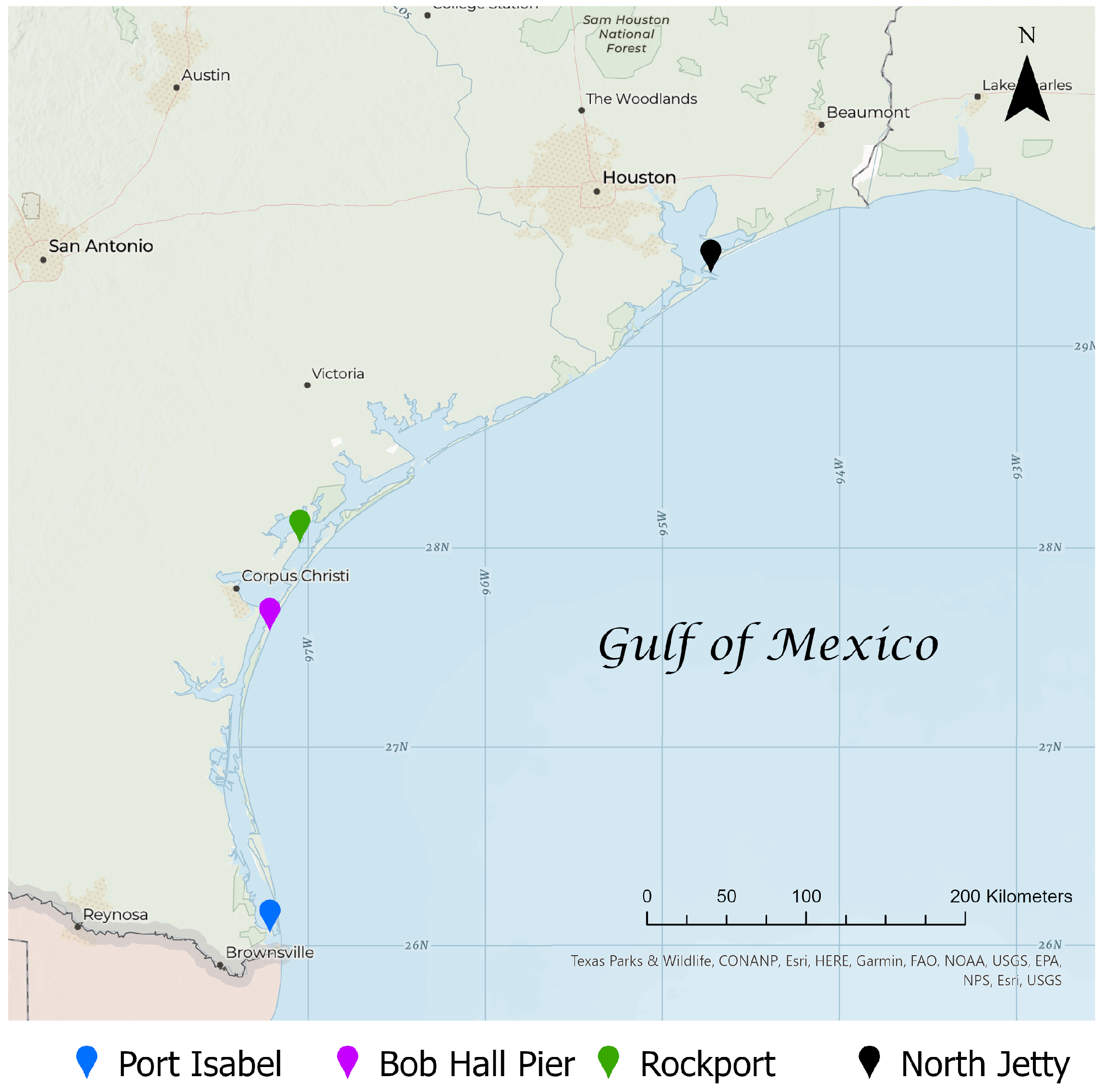
The four tide gauge stations illustrated in
Figure 1 were selected to represent the diverse metocean conditions along the Texas coast in the Gulf of Mexico. From south to north, these stations are Port Isabel, Bob Hall Pier, Rockport, and Galveston Bay Entrance, North Jetty. These locations are important due to their proximity to the major ship channel ports of Houston/Galveston (North Jetty) and Corpus Christi (Bob Hall Pier), which rank first and third in the U.S. by tonnage, respectively (United States Army Corps of Engineers, 2023), as well as the Port of Brownsville (Port Isabel). Additionally, these tide gauge stations are near recreational beaches (Bob Hall Pier and North Jetty), a NOAA National Estuarine Research Reserve (Rockport), and sensitive coastal ecosystems (all stations).
Some of the characteristics of the respective tide gauge stations are listed in
Table 1, along with local metocean conditions. The Great Diurnal Tidal Ranges (GDR) is the height difference between the mean higher high water and the mean lower low water [
31]. While the Texas coast is microtidal [
32], the GDR varies substantially along the Texas coast, from non-tidal in the Laguna Madre [
33] to about 0.5 m for locations along the GOM coast such as Bob Hall Pier, an open coast location, and North Jetty, a station protected by a long jetty at the entrance of the Houston ship channel. The other two stations, Port Isabel and Rockport, are more inland. Their water level variability is attenuated depending on the hydraulic resistance between the coast and the tide gauges’ respective locations outside of extreme event conditions. The GDRs of Port Isabel and Rockport are 0.41 m and 0.11 m, respectively. Further inland, the station of Port Isabel is along a deep ship channel (12.8 m [
34]), resulting in a less attenuated water level range than that of Rockport. Note that the GDR will also influence the accuracy of water level predictions, with larger water level variability typically resulting in larger prediction errors and a more challenging task to meet the NOAA criterion of a CF (15 cm) greater than 90%.
The short-term water level dynamic also varies depending on location. Each selected station experiences different wind and wave climates, resulting in part from a growing distance to the continental shelf for the more northern stations. The mean wind speeds along the Texas coast are some of the highest in the continental US and vary from 4.9 m/s to 6.1 m/s for our study sites depending on the location’s including distance from the open coast. Strong winds lead directly or indirectly, through their influence on alongshore coastal currents, to higher or lower water levels both along the shores of the GOM and within the bays and estuaries, depending on the wind direction. Large waves along the coast lead to higher water levels and runup on open ocean beaches. Occasional extreme events can result in significant changes in water levels, as exemplified by the impacts of Hurricanes Hanna in 2020, Harvey in 2017, and Ike in 2008. These events caused substantial damage, including the destruction of Bob Hall Pier by Hurricane Hanna, the disabling of the Rockport station during Hurricane Harvey, and the widespread devastation caused by Hurricane Ike. Although extreme events influence the performance of the models, these low-frequency extreme events are not part of the scope of this study. The proposed work aims to design a deep learning-based method to predict water levels that can perform well in multiple locations independently of the described differences between these stations.
2.2. Dataset
The dataset utilized for this research combines 6 min data sourced from NOAA Tides and Currents [
35] and data from the Texas Coastal Ocean Observation Network (TCOON) [
36], accessible via the Texas Digital Library TCOON Collection [
37]. While the water level, harmonic prediction, and surge data were sourced from NOAA, the wind data were sourced from TCOON historical records and made available on GitHub. This multi-source data approach was adopted to enhance data quality and minimize missing values, addressing gaps ranging from 6 min to several months in both the wind and water level datasets.
One challenge in using environmental data for machine learning applications is acquiring high-quality data with minimal missing values, ensuring that the overall dataset distribution remains unaffected. To mitigate this issue, we devised a data preprocessing methodology to address missing values (refer to
Section 2.2.2), evaluated in Section Evaluation of the Gap-Filling Approach Used. We identified the years with the fewest missing values across combined variables for each location. To maintain data distribution integrity, we only selected the years where less than 2% of 6 min observations were missing, resulting in varying years chosen for different stations. Subsequently, we proceeded to the data preprocessing stage, preparing the data for the neural network (refer to
Section 2.2.3).
2.2.1. Inputs
The selection of inputs depends on the research objectives, the dynamics of the system, and, particularly for operational models, data availability. While theoretical research often considers numerous variables, operational studies are limited to existing real-time data and favor fewer inputs to limit sensitivity to data consistency challenges, especially during extreme events. This research aims to implement the proposed model in real-time, so only past surges (surge = water level − harmonic prediction) and measured and predicted wind along and across the shore were utilized as inputs, with the surge variable used as the target. Using surge rather than water level as the input and target improves the model’s performance by decoupling the tidal signal, driven by gravitational forces, from metocean forcings. The tidal component is subtracted from the water level signal before being fed into the model, and it is added back to the predictions to obtain complete water level predictions.
The wind data used in this study were collected by sensors installed at the tide gauge stations. The wind observations include both wind direction and speed, which were converted into alongshore and across-shore wind components. This conversion was necessary before using the wind data as AI model inputs, as the model cannot inherently understand that 0 and 360 degrees represent the same direction. This preprocessing step ensured that the model could effectively interpret the wind data.
2.2.2. Data Preprocessing
The data preparation step resulted in a high-quality dataset by minimizing the number of gaps, resulting in the AI-ready data available in the GitHub repository. The gap-filling process was divided into two stages: addressing short and long gaps. A short gap was defined as one lasting up to 1 h for wind data and 3 h for surge values. Any gaps exceeding these durations were classified as long gaps. While only short gaps were identified in the water level time series, both short- and long-term gaps were observed in the wind time series. Surge values were utilized to fill gaps in water levels, while along-shore and across-shore values were employed to fill gaps in wind data.
NOAA employs a post-processing approach to fill most of the water level gaps [
5]. Consequently, the NOAA-verified water level time series quality was excellent, with only a few short gaps to fill, typically averaging about an hour per year per station due to station maintenance. In contrast, NOAA does not apply post-processing corrections to the wind data, resulting in a significant number of missing values, with some gaps spanning from multiple days to months. The TCOON wind data exhibited fewer missing values compared to the NOAA wind data and hence was selected. Large gaps were filled using a correction based on the NOAA dataset when those data were available.
The short gap-filling process, applied to both surge and winds, involved applying a linear interpolation approach. The interpolation began with computing the average of the five 6 min values preceding the gap as the starting value and concluded with averaging the first five values following the gap as the end value. Utilizing an average value computed over thirty minutes before and after the gaps enhanced the robustness of the gap-filling approach.
The long gap-filling process for the wind time series involved integrating data from both NOAA and TCOON. Although the data from NOAA and TCOON originated from the same wind sensor at each location, they often exhibited a different number of missing values due to variations in post-processing approaches before public release. To address this inconsistency, a replacement approach with correction was implemented. An average of the previous five values before the gap and the first five values at the end of the gap were computed for both the NOAA and TCOON data. The discrepancies between the values from both data sources before and after the gap were calculated. The average of these differences served as the correction value, which was then added to the data from the other source to fill the long gaps.
Evaluation of the Gap-Filling Approach Used
To assess the robustness of the proposed gap-filling approaches and ensure that the data distribution remained unchanged, artificial gaps were created in a test dataset. Subsequently, these gaps were filled using the described methods, and the accuracy assessed based on the Mean Absolute Error (MAE) [
38] and Root Mean Squared Error (RMSE) [
38] (refer to Equations (
1) and (
2)). The metrics reported in
Table 2,
Table 3 and
Table 4 are based on thirty repetitions, with about 40% of the data being successively removed for gaps of varying lengths for each repetition. The MAE and RMSE statistics were computed across all gaps, while the standard deviations (SDs) reflect the variability across the thirty repetitions.
where
and
are the true measurements and the gap-filled values, respectively.
The analysis of the results in
Table 2 reveals the effectiveness of the proposed short gap interpolation method. Across all stations, both the MAE and RMSE for the surge values remain below 3.8 and 5.0 cm, respectively. Notably, the 3.8 cm threshold meets the 15 cm NOAA CF standard.
Table 3 presents the results of interpolating short gaps in wind data, demonstrating the success of the proposed interpolation approach.
Table 4 illustrates the error associated with filling long gaps in the wind data. The remarkably low errors in the table can be attributed to the utilization of data from two datasets originating from the same sensor despite undergoing different post-processing methods. This enables a highly accurate gap-filling method for handling long gaps.
2.2.3. Data Preparation
The data preparation step involved formatting the dataset to be used as a neural network input. However, despite employing the gap-filling method, some gaps remained unfilled, leading to an incomplete time series and posing a significant challenge. In environmental time series problems, it is widely known that previous time steps contain valuable information that contributes to better predictions. Hence, we incorporated columns containing past wind and water level measurements. Specifically, we included hourly measurements ranging from the current time up to 12 h prior for 12, 24, and 48 h predictions, as well as up to 6 h prior for 72 and 96 h predictions, for both water level and wind variables. The selection of prior measurement windows varies depending on forecast times, driven by the evolving dynamics of water level predictions. As the lead time increases, the significance of wind predictions becomes more pronounced, while the importance of past wind and water level measurements diminishes. Furthermore, hourly columns were included for the wind-perfect prognosis technique, spanning from the forecast time to the predicted time. Subsequently, after creating all the necessary columns, rows containing missing values were removed.
2.3. Methodology
The growing power of deep learning techniques has revolutionized various fields, including environmental science and hydrology. These advanced methods are particularly adept at handling complex, non-linear relationships within large datasets, offering the potential for significantly improved predictive performance over traditional approaches [
39]. By leveraging long-term historical data and utilizing modern techniques to control overfitting [
40], deep learning models can provide more accurate and reliable predictions.
This research aimed to evaluate and compare the performance of several state-of-the-art deep learning architectures for the prediction of coastal water levels. The architectures compared included MLP [
41], Seq2Seq [
42], transformer [
43], conformer [
44], and informer [
45]. While the methodology section focuses on the detailed description and implementation of the Seq2Seq architecture (
Section 2.3.1), which was found to perform best for our specific problem, the section also includes a discussion of harmonic analysis as the baseline standard for water level prediction (
Section 2.3.2). Descriptions of the other deep learning architectures are provided in
Appendix A.
An initial set of hyperparameters was determined using KerasTuner for each deep learning architecture. Further tuning was conducted by the modeler, focusing on learning curves and other performance metrics. Various sets of hyperparameters were tested across different locations and lead times for each architecture. However, the models’ performances did not show significant differences with varying hyperparameter settings. Therefore, a single architecture and a consistent set of hyperparameters were selected for each DL method. The models utilized the Adam optimizer [
46] and mean squared error as the loss function [
47]. They incorporated a learning rate scheduler with a reduction factor of 0.1 and a patience of 10 epochs. Additionally, early stopping was implemented with a patience value of 35 epochs, a learning rate set to 0.0001, and a batch size of 512.
2.3.1. Seq2Seq
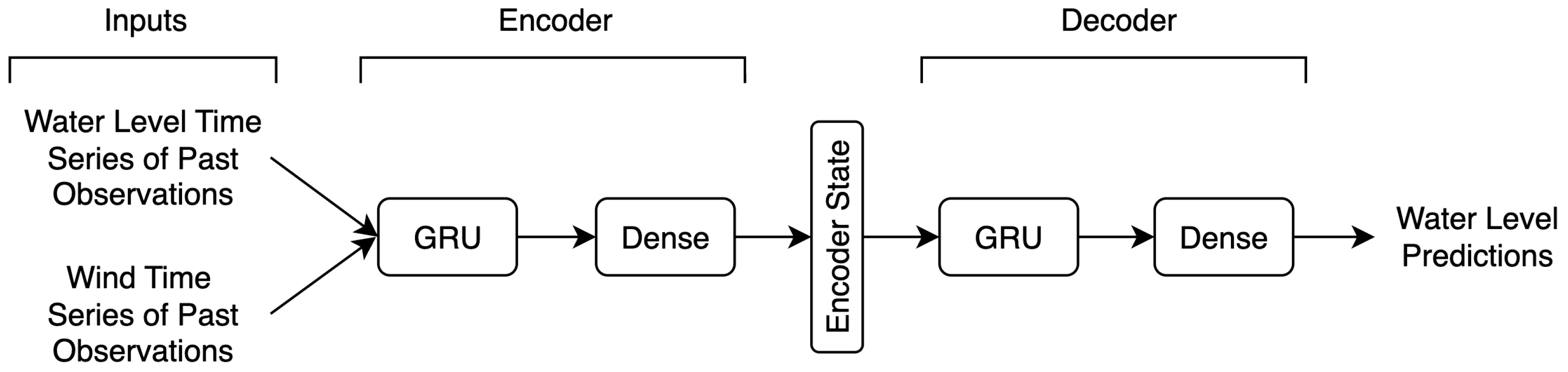
The Seq2Seq architecture, also known as the encoder–decoder architecture, is a neural network model designed for handling sequences of varying lengths [
42]. Seq2Seq architectures are highly versatile and can be adapted for various tasks by changing the input and output data. They have been extended and improved with variations such as attention mechanisms, which allow the model to focus on different parts of the input sequence during decoding, resulting in better performance, especially for longer sequences.
The encoder is the first part of the Seq2Seq model. It takes an input sequence of variable length and encodes it into a fixed-size context vector or hidden state. This context vector is meant to capture the semantic information from the input sequence. The encoder is typically implemented using a Recurrent Neural Network (RNN), Long Short-Term Memory (LSTM), or Gated Recurrent Unit (GRU). The input sequence is processed one token at a time, and the hidden state is updated at each step [
42].
The decoder is the second part of the Seq2Seq model. It takes the context vector produced by the encoder as its initial hidden state and generates an output sequence one token at a time. Similar to the encoder, the decoder is typically implemented using an RNN, LSTM, or GRU. During training, the decoder is provided with the target sequence (the ground truth), and it generates tokens to match the target sequence [
42].
Seq2Seq models are trained using pairs of input and target sequences. The encoder processes the input sequence, and the decoder generates the output sequence step by step. The loss is computed by comparing the predicted sequence with the target sequence, and backpropagation is used to update the model’s parameters [
42].
After an extensive hyperparameter tuning process using KerasTuner, the Seq2seq model architecture was defined. The encoder utilized a GRU layer with 1 unit, configured with a tanh activation function and dropout for regularization, followed by a dense layer with 32 units using tanh activation. The decoder employed a GRUCell with 32 units, capable of predicting sequences, and featured an optional attention mechanism with configurable sizes and dropout (refer to
Figure 2). The model was optimized using the RMSprop optimizer with a learning rate of 0.0001 and mean squared error as the loss function. Early stopping with a patience of 40 epochs and a batch size of 512 was used to ensure high performance and prevent overfitting.
2.3.2. Harmonic Analysis
The performance of all the models was compared with tidal predictions [
48]. Tidal predictions can be computed years in advance; however, they do not account for relative sea level rise, weather, or other environmental factors. Tidal predictions for the respective locations and years were obtained from the NOAA Tides and Currents station pages. NOAA tidal predictions are referenced to the last tidal epoch (1983–2001) for the stations at Port Isabel, Bob Hall Pier, and North Jetties. For Rockport, a later reference period (2002–2006) was used by NOAA (NOAA CO-OPS). Zero mean sea level was computed based on these epochs, so the performance of tidal predictions decreases over time due to relative sea level rise. To better compare the predictive methodologies, the following rates of relative sea level rise for the study locations were considered: Port Isabel = 4.29 mm/year [
49], Bob Hall Pier = 5.48 mm/year [
50], Rockport = 5.97 mm/year [
51], and North Jetty = 6.32 mm/year [
52]. For each location, the difference from the midpoint of the tidal epoch was multiplied by the station’s rate of relative sea level rise, and the result was added as a bias adjustment to the station’s tidal predictions. The same metrics were then used to compute the performance of these adjusted tidal predictions. Using tidal predictions without these corrections would result in a lower performance and would not provide a fair comparison of the respective methodologies.
3. Results and Discussion
AI models have uncertainty due to the selection of different local minima during repeated calibrations. To confidently evaluate model performance, it is best to train and assess the performance of the models multiple times. In our study, each model was trained five times, and their performances were compared by considering the respective metric ranges. From these five runs, the model with the median performance for the CF of 15 cm was selected as the representative model for that architecture. This representative model was then used to compare performance across different architectures while accounting for the performance ranges.
For environmental problems, it is also necessary to consider year-to-year variability, since a model may perform better in some years than others. A model that performs consistently well over multiple years demonstrates the desired robust generalization. To assess year-to-year variability, five years of data were used for each location, along with a K-Fold validation approach [
53]. A one-year timespan was selected for each fold to capture the seasonal variability in water levels. The experimental design resulted in the model’s performance being assessed over five independent testing sets. For each fold, the validation dataset included three months of data from each of the remaining four years, resulting in a year of data, while the training dataset consisted of the remaining three years of data. For each of the five forecast times and four locations, and for each of the five architectures, the models were trained five times, resulting in a total of 3000 individual models once the respective architectures were established through the tuning process described in
Section 2.3.
The metric used for evaluating the model’s performance is the CF of 15 cm, which calculates the percentage of predicted values with an absolute error of 15 cm or less. A higher CF indicates more accurate predictions, as it means a greater proportion of values have an error of 15 cm or smaller. Additionally, for a water level predictive model to be considered operational, the NOAA requirements include that its CF of 15 cm be 90% or higher.
3.1. Performance Comparison of the Deep Learning Architectures
This section evaluates the performance of the proposed architectures across all lead times, locations, and test years, aiming to determine the best-performing architecture for short-term water level predictions. To ensure a robust comparison, we analyzed the median performance from five training repetitions for each case, focusing on the CF (15 cm) metric. This metric was selected because a model achieving 90% or higher CF (15 cm) is required for operational use. It emphasizes the model’s performance while emphasizing low-frequency and high-impact events.
Table 5 presents the architecture that performed best overall across the five independent testing years when comparing the median performance of the respective models. The median performance was selected for comparison to improve the robustness of the results, although the range of performance for the five repetitions was typically small. To be considered the best model, the CF (15 cm) of the median model had to be the largest of the five models more frequently than the other models. The higher performance was typically observed for two or three of the test years. If two architectures are listed, it indicates a tie, i.e., the two architectures were the top performers for two of the testing years, with no single architecture emerging as the best for that specific location and lead time.
Table 5 shows that the Seq2Seq model demonstrates the best performance in most scenarios. Out of twenty-five combinations, Seq2Seq was the top performer in ten and tied for the best in six. The MLP architecture was the second-best, being the top or tied across six scenarios. Overall, based on the CF (15 cm) metric, Seq2Seq emerged as the top-performing architecture for this research problem. The detailed results can be found in
Appendix B.
Further analysis of
Table 5 reveals that Seq2Seq performed the best for Bob Hall Pier and Rockport for all lead times. For Port Isabel, Seq2Seq was the best for all lead times except for the 12 h predictions, where the transformer architecture outperformed it by less than 0.1% for the respective CF (15 cm) median cases. At North Jetty, Seq2Seq’s performance was, on average, within 0.8% of the best-performing architecture, which varied by lead time. Although Seq2Seq was not the top performer or tied for the best in five out of twenty locations and lead times, its performance was consistently among the highest based on the CF (15 cm) metric. Overall, Seq2Seq emerged as the best-performing model for predicting water levels along the Texas coast. While the selection of Seq2Seq as the best performing model was based on a robust range of test years, architectures, and hyperparameters, it should be emphasized that differences in CF (15 cm) are not that large between models. These differences can be summarized by comparing the range of the worst- and best-performing models for the five test years for all lead times combined, 12 h to 96 h. The performance differences range from 3.0% to 5.5% for North Jetty, 1.0% to 8.8% for Rockport, 0.8% to 2.2% for Port Isabel, and 1.3% to 4.8% for Bob Hall Pier.
If metrics more focused on overall performance, such as MAE or RMSE, had been selected, the rankings of the models based on their median performance would have differed, and no single model would consistently show the best performance. However, when using CF (15 cm), the Seq2Seq architecture consistently demonstrated superior performance (refer to
Table 5) across all locations except North Jetty. The results in this table are derived from the median repetitions found in
Appendix B.
Table A1 illustrates the results for Bob Hall Pier, showing that Seq2Seq was the best-performing architecture in 16 out of 25 experiments, clearly establishing it as the best architecture. Similarly, for Port Isabel (refer to
Table A2), Seq2Seq was the best in 15 out of 25 cases. For Rockport (refer to
Table A3), it was the best-performing architecture in 19 out of 25 cases. For North Jetty (refer to
Table A4), Seq2Seq showed the best performance in 10 out of 25 cases. Thus, Seq2Seq emerges as the best architecture across all locations.
Another important observation from
Table A1,
Table A2,
Table A3 and
Table A4 is that although Seq2Seq was the best-performing architecture, the performance of the second-best architecture, often either the MLP or transformer, was very similar in terms of CF (15 cm). For instance, at Bob Hall Pier, Seq2Seq outperformed the second-best architecture by an average of only 0.2% for the 12 h predictions. These small performance differences were maintained for the 24 h, 48 h, 72 h, and 96 h predictions, with differences of 0.3%, 0.3%, 0.3%, and 0.4%, respectively. These small performance differences between the best and second-best median models were consistent across the other locations, including Port Isabel, Rockport, and North Jetty.
Table 6 illustrates the Seq2Seq median results of the respective five independent testing years for the different stations and lead times. The Seq2Seq model met NOAA’s operational standards for predictions of up to 96 h for Port Isabel and Rockport and up to 72 h for Bob Hall Pier. This represents a substantial improvement compared to the state-of-the-art in the literature, which was unable to meet the CF criterion for predictions beyond 48 h [
28,
54]. The performance for Bob Hall Pier was inferior compared to the other two stations due to the larger water level range on the open coast, which makes predictions more challenging. In contrast, the inland stations, which exhibit attenuated water level ranges, showed higher performances. Additionally,
Table 6 shows a lower performance for the North Jetty location. Despite being protected by jetties, this station is on the open coast and experiences minimal attenuation, resulting in a water level range similar to that of Bob Hall Pier. The more northern station of North Jetty is correlated with a wider offshore continental shelf, making it more sensitive to wind forcings compared to the southern locations where deep waters are closer to the coastline. This increased sensitivity to metocean forcings makes predictions more challenging, explaining the lower performance.
Furthermore,
Table 6 presents the median tidal prediction CF (15 cm) for the same set of testing years as
Table 5. Despite the relative sea level rise adjustment, none of the tidal predictions met the NOAA criterion for operational water level prediction models of CF (15 cm) > 90%. The importance of wind forcing along the continental shelf is reflected in the North Jetty tidal predictions performance, which stands at 71.8%. For all locations and testing years, the performance of the harmonic tidal predictions was lower than the 96 h Seq2Seq predictions, confirming the ability of the AI model to integrate atmospheric forcings and provide more accurate water level predictions.
MLPs are not specifically designed to handle sequential data. Although MLPs can model very complex functions, their architecture is not tailored to capture temporal interdependencies at multiple time scales. Similarly, transformer architectures, despite their self-attention mechanisms, are not inherently designed to capture temporal dependencies. They are more focused on capturing long-range dependencies, which may not align with the specific temporal patterns present in water level time series data.
During the hyperparameter tuning process, it was observed that using a large number of attention heads in the transformer architectures led to overfitting despite mitigating the potential for overfitting by using dropouts and regularization. While the multi-head attention mechanism does not inherently cause overfitting, it introduces additional complexity to the model. This increases the likelihood of overfitting, especially in cases where the problem is characterized by low dimensionality and relatively straightforward relationships, such as water level predictions.
The Seq2Seq architecture emerged as the best-performing model for predicting water levels based on the CF (15 cm) metric. This is likely due to a good balance between sufficient complexity to capture the nonlinear relationships between metocean forcings and future water levels while maintaining a relatively simpler architecture that is sufficient to capture the relationships between the limited number of predictors and the target of this problem. These relatively simple interdependencies may pose a challenge for more complex architectures, such as the informer, conformer, and transformer architectures, as they will be more prone to overfitting. And, the Seq2Seq model’s inherent ability to more explicitly extract temporal dependencies at different timescales likely explains its superior performance compared to simpler MLP architectures.
3.2. Analysis of the Yearly Variability of the Predictions
Understanding year-to-year variability is essential for assessing how well the model generalizes to different datasets and future years.
Figure 3 illustrates this variability by showing the CF (15 cm) results for the Seq2Seq architecture. Each dot represents the median value of the five independent testing years, while the tips of the error bars indicate the performance for the best and worst testing years.
Figure 3 highlights the overall excellent performance of the Seq2Seq architecture, with all stations achieving at least 90% for 12 and 24 h predictions except for one year for 24 h predictions at North Jetty. For Port Isabel and Rockport, model performance was consistently above 90% for 48 h predictions and for all but one year for 72 h predictions. The median results for 96 h predictions also surpassed the 90% threshold, demonstrating the potential for longer lead time predictions with this approach.
The error bars in
Figure 3 indicate that the performance difference across independent testing years is relatively consistent for short lead times but increases with longer lead times. As discussed in
Section 2.2.3, the importance of the past measurements decreases with lead time, as evidenced from the smaller number of past measurements in the optimized architectures of the longer lead time predictions. Hence, short-term water level predictions will be more influenced by recent anomalous high or low water levels. In contrast, longer lead time predictions of 48 h and beyond rely more on wind predictions and less on historical water level data. This likely makes it more challenging to adjust for anomalous average water levels, resulting in an asymmetrical 5-year range for the performance metrics of long lead time predictions. Since tidal predictions lack direct measurements, adjustments for unusually high or low water levels are not feasible, leading to the lowest performances and wider ranges of CF (15 cm) observed in the figure.
For all models that included 2010 as a test year, for all locations except North Jetty, the lowest performance was recorded during that period. This particular year was marked by historically unusual water levels along the Texas coast. In the case of North Jetty, the lowest performance occurred in 2016: another year characterized by significant interannual variability, though it was less pronounced than in 2010. The difference in performance for the worst-performing year impacts performance in two different ways. The inclusion of the testing year in the training set provides an advantage by exposing the models to a wider range of average water level conditions. When the challenging year is not included, the models trained on the rest of the data will have more difficulties predicting under somewhat different conditions, leading to lower performance as well. The performance distributions for Rockport across all lead times appeared to be more symmetrical compared to the other stations, with the lowest performance still occurring in 2010, as anticipated. This may be attributed to Rockport having a substantially smaller GDR, resulting in smaller average water level differences compared to other locations. Consequently, past water levels likely played a more crucial role for longer lead times at this station, enabling the models to better accommodate unusually high or low average water levels.
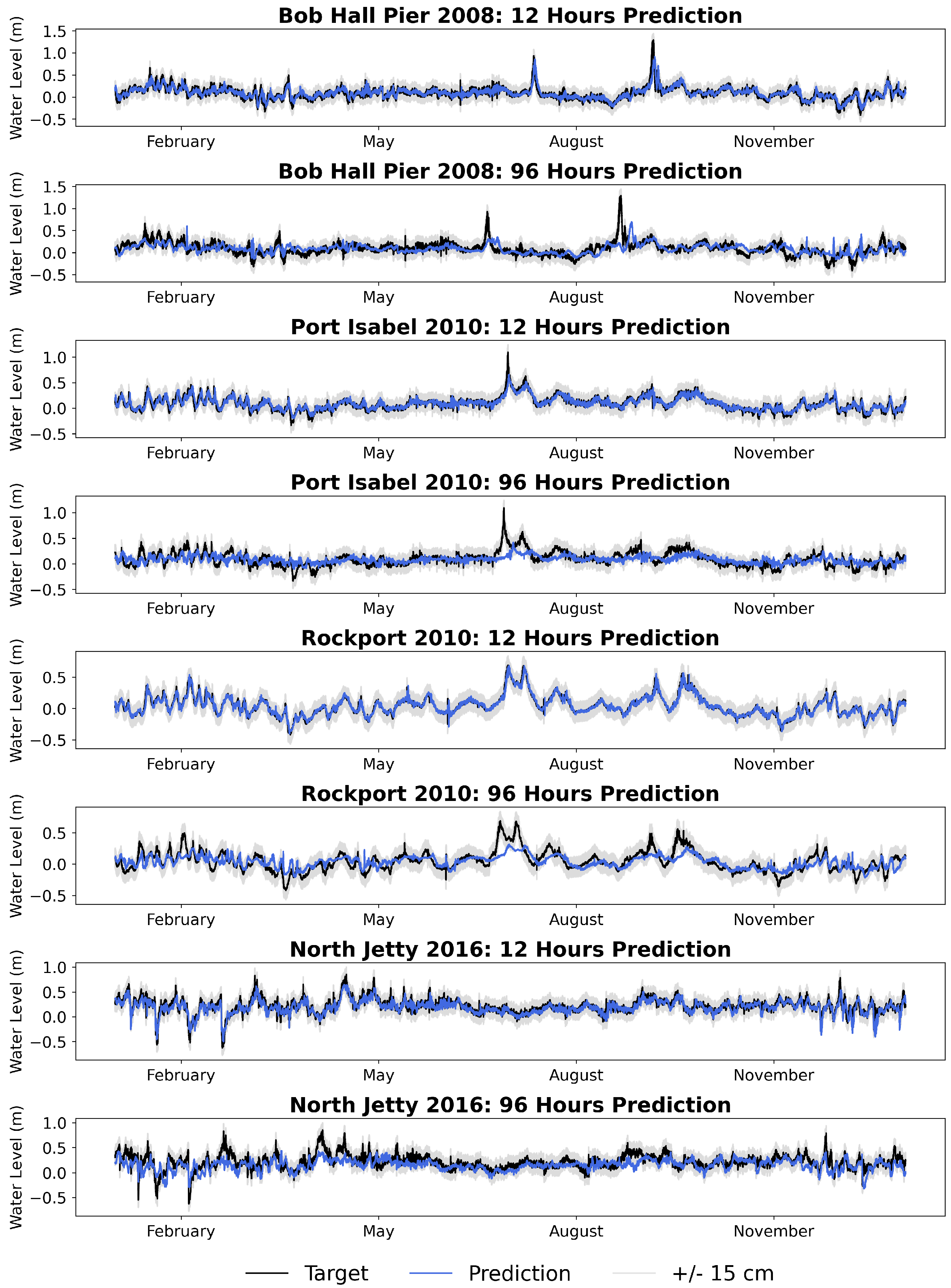
The impact of these unusual years on average water levels, specifically 2010 and 2016, is also reflected in
Figure 4. This figure presents a time series of predictions for 12 and 96 h lead times for the year that resulted in the lowest performance at each location, except for Bob Hall Pier, where 2008 was selected due to the influence of hurricanes Dolly and Ike on the predictions.
The Oceanic Niño Index (ONI) for the Niño 3.4 region is typically used to characterize conditions, with 3-month running mean sea surface temperatures above 0.5
∘C indicating an El Niño event and below −0.5
∘C indicating a La Niña event [
55]. The year 2010 was particularly unusual, as it started with strong El Niño conditions (ONI for December–January–February = 1.5) and ended with strong La Niña conditions (ONI for November–December–January = −1.6) [
55]. El Niño and La Niña are the two phases of the well-known climatic variability observed in the Pacific Ocean, which significantly influences weather patterns globally.
The El Niño–Southern Oscillation (ENSO) shift in 2010 was compounded by a loop current eddy colliding with the Texas coast in July of that year. Such events typically lead to an increase in average water levels of about 15 cm [
56]. This contributed to one of the largest yearly interannual variability values in water levels, approximately 35 cm, observed along the Texas coast since records began in 1908 [
52].
All stations tested for 2010 (Bob Hall Pier, Rockport, and Port Isabel) were trained on data from other years that did not experience such significant changes in average water levels, which explains the somewhat lower performance for that year. For the North Jetty station, the performance of the deep learning model was lower in 2016; a year that also experienced large changes in ENSO conditions. The ONI (DJF) for 2016 was 2.5, and it ended the year with an ONI (NDJ) of −0.6. This resulted in an interannual variability range of about 25 cm, making it more challenging for models trained on data from other years to make accurate predictions.
For all cases, the performance of the 12 h predictive models was significantly better than the 96 h predictions, as expected, with the vast majority of the predictions falling within the ±15 cm range. The 96 h comparative graphics allow us to observe the conditions leading to predictions outside this ±15 cm range. For all locations, the majority of the discrepancies involved several hours of predictions above or below that range during sharp changes in water levels, such as the passage of cold fronts (resulting in low water level events) or strong southerly winds (resulting in high water level events).
In addition to the interannual variability, the Texas coast was significantly impacted by several tropical storms and hurricanes in 2008, with Hurricanes Ike and Dolly making landfall that year. These intense but short-duration storms had a substantial impact on model performance over 2–3 days. This impact can be observed in
Figure 4 for Bob Hall Pier, particularly for the 96 h predictions. During these periods, the predictions fall outside the ±15 cm range for several hours, which lowers the overall performance of the models. It should be noted that these models are not designed to predict water levels during tropical storms or hurricanes. A larger number and variety of the impact of such storms on water levels and metocean conditions would need to be recorded to make the calibration of AI models for such conditions promising.
3.3. Exploring Extended Water Level Predictions: A Case Study of 108-Hour Forecasts for Port Isabel and Rockport
The goal was to create a generalizable model that is applicable across diverse locations along the Texas coast while extending the lead time of model predictions, currently meeting NOAA’s standard for CF (15 cm) for up to 48 h [
28]. The analysis revealed that employing the Seq2Seq architecture allowed the predictions to be extended up to 96 h into the future for most of the studied locations while still meeting the NOAA standard for CF (15 cm).
The predictability and dynamics of weather forcings significantly influence model performance, posing challenges for longer-term temporal predictions. Inland stations such as Port Isabel and Rockport exhibit reduced water level ranges, facilitating predictions within the ±15 cm range and enabling longer lead times. Consequently, a case study was conducted on these locations to explore the feasibility of further extending water level predictions. The case study revealed that, for these two locations, it was possible to maintain the 90% CF of 15 cm for most of the independent testing years up to 108 h (refer to
Table 7) using the Seq2Seq model.
The low performance for Port Isabel for Year 3 and for Rockport for Year 2 correspond to the very unusual year of 2010. Rockport Year 1 (2009) also showed a lower performance, while Years 3 and 4 showed performances substantially above 90%. Coupling the present deep learning predictions with subseasonal-to-seasonal water level predictions has the potential to account for unusual conditions (e.g., ENSO-driven events) and significantly improve performance, potentially leading to CF (15 cm)-compliant predictions for even longer lead times.
3.4. Practical Applications and Model Limitations
In this section, we expand on the broader implications of applying deep learning models, such as Seq2Seq, to predict water levels in different coastal environments. While our study focused on the Gulf of Mexico, a microtidal region with strong metocean forcings, the potential for applying this model in other coastal areas, including macrotidal environments, is worth discussing. Below, we address key considerations related to the model’s general applicability, particularly in environments with differing tidal dynamics.
3.4.1. Applicability and Potential of Seq2Seq in Coastal Water Level Predictions
Our research demonstrated the Seq2Seq model’s effectiveness for water level predictions in the Gulf of Mexico, a microtidal region. However, coastal environments vary significantly, and different locations may require adaptations of the model to account for varying atmospheric and oceanic conditions. In macrotidal environments, tidal ranges are much larger. However, other metocean forcings may still be important for the accurate predictions of water levels. even if differences with tidal predictions represent a smaller proportion of the overall water level variability. The primary drivers of water levels and their potential interactions with the larger tidal range will be somewhat different than for a microtidal environment, which could lead to the need for additional inputs and research to validate the model’s adaptability and performance in such regions.
While our study focused on different locations within a specific geographic region, the Seq2Seq model provides a flexible framework that could be applied globally, including for locations with the metocean conditions discussed above. The Seq2Seq architecture’s ability to handle complex, nonlinear relationships between variables, such as wind speed, wind direction, and water level fluctuations, makes it suitable for other coastal regions. Other input variables can easily be added as model inputs, and Seq2Seq is a relatively computationally efficient architecture compared to other more complex DL architectures.
Even though our model does not explicitly isolate extreme wind speeds as a variable, it was trained using a dataset that included several instances of strong winds exceeding 20 m/s, allowing the model to incorporate the impact of strong winds on water levels. ML models learn based on past data, and hurricane-force winds were not part of this dataset. Hence, the model should not be used in these extreme and rare conditions. Furthermore, wind speeds and directions can fluctuate dramatically as the eye of a hurricane impacts a coastal region. As it would take several hurricanes of different strengths, paths, sizes, or a set of realistic synthetic equivalents of hurricanes to impact the model location, the authors do not foresee this type of ML approach to be effective in such rare cases. However, this is not seen as a limitation, as coastal regions are evacuated and the most stringent precautionary measures are taken ahead of the impact of a hurricane. The present models are designed to assist coastal managers in all other types of situations, including the fast-increasing occurrence of sunny day floods.
3.4.2. Importance of 96 h Predictions for Coastal Management
One of the key advantages of our model is its ability to forecast up to 96 h into the future. This capability is particularly important for coastal management and planning. Although tide tables perform better under calm conditions, their accuracy diminishes when wind forcing becomes significant, especially in regions like the Gulf of Mexico. The accuracy of tide tables is also affected by the inter-annual variability and the timing of the seasonal shifts of sea levels at the location. Along the shores of the Gulf of Mexico, the inter-annual variability and the seasonal variability of water levels are similar to the tidal range, all around or below 30 cm [
35]. By including real-time water levels and wind measurements, our Seq2Seq model offers an enhanced prediction capability that accounts for tidal elevation, inter-annual fluctuations, seasonal adjustments, and wind effects, providing critical information for coastal activities. The ability to predict up to 96 h ahead allows coastal stakeholders to better prepare for potential disruptions caused by strong winds or other atmospheric conditions. This predictive range offers a more comprehensive decision-making tool, particularly for managing shipping, port operations, and coastal infrastructure in the face of changing weather conditions.
4. Conclusions
The results showed that the Seq2Seq architecture achieved the best performance for predicting water levels across multiple locations in the Gulf of Mexico based on the CF (15 cm) metric, the most widely used criterion regarding the predictions of water levels for navigation, tide gauges, and other impactful events. Seq2Seq outperformed the other models for most locations and lead times, and its performance was within 1% of the top-performing architectures in cases where it was not the best. The analysis indicates that, for all locations except North Jetty, it was possible to make 72 h predictions while maintaining NOAA’s CF (15 cm) standards. Furthermore, the Port Isabel and Rockport stations were able to maintain these standards for up to 108 h for most of the independent testing years. This represents a significant improvement over the existing literature, which had not achieved NOAA’s standards beyond 48 h.
The proposed AI water level prediction models can be computed almost instantly once trained and optimized, and the models were recently implemented operationally (
https://sherlock-prod.tamucc.edu/cbocp/, accessed on 7 October 2024). Ongoing work aims to extend these predictions from average water levels to a coastal inundation model. This new model leverages the flexibility of AI to incorporate additional inputs such as local wave measurements and predictions. The goal is to predict the vertical height that water will reach on the beach, including runup, to provide more precise information to stakeholders regarding the probability of coastal inundation.
One of the current limitations of this research is the presence of missing values in the dataset, particularly in the wind observations. A more complete dataset with fewer missing values would allow for the inclusion of additional years in the training set, potentially improving the model’s performance. However, we have implemented an interpolation method that enabled us to utilize five years of data, which has proven sufficient to achieve strong predictive performance.
Future work will focus on the development of location-specific models for tide gauge stations. While our current study developed a generalized model that performs well across multiple locations, creating specialized models tailored to each specific site could further enhance performance. These specialized models would consider the inclusion of water level data from nearby stations, which may have correlations or temporal lags that could contribute to more accurate predictions.


