
Appraisal of Daily Temperature and Rainfall Events in the Context of Global Warming in South Australia

 ,
,
Abstract
1. Introduction
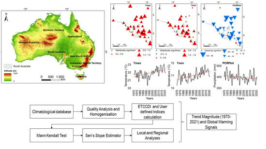
2. Materials and Methods

| Index ID | Index Name | Definition | Units |
|---|---|---|---|
| Temperature indices-User defined | |||
| Tmax | Maximum temperature | The annual mean value of daily maximum temperature for the period 1970–2021 | °C |
| Tmin | Minimum temperature | The annual mean value of daily minimum temperature for the period 1970–2021 | °C |
| Extreme hot temperature events | |||
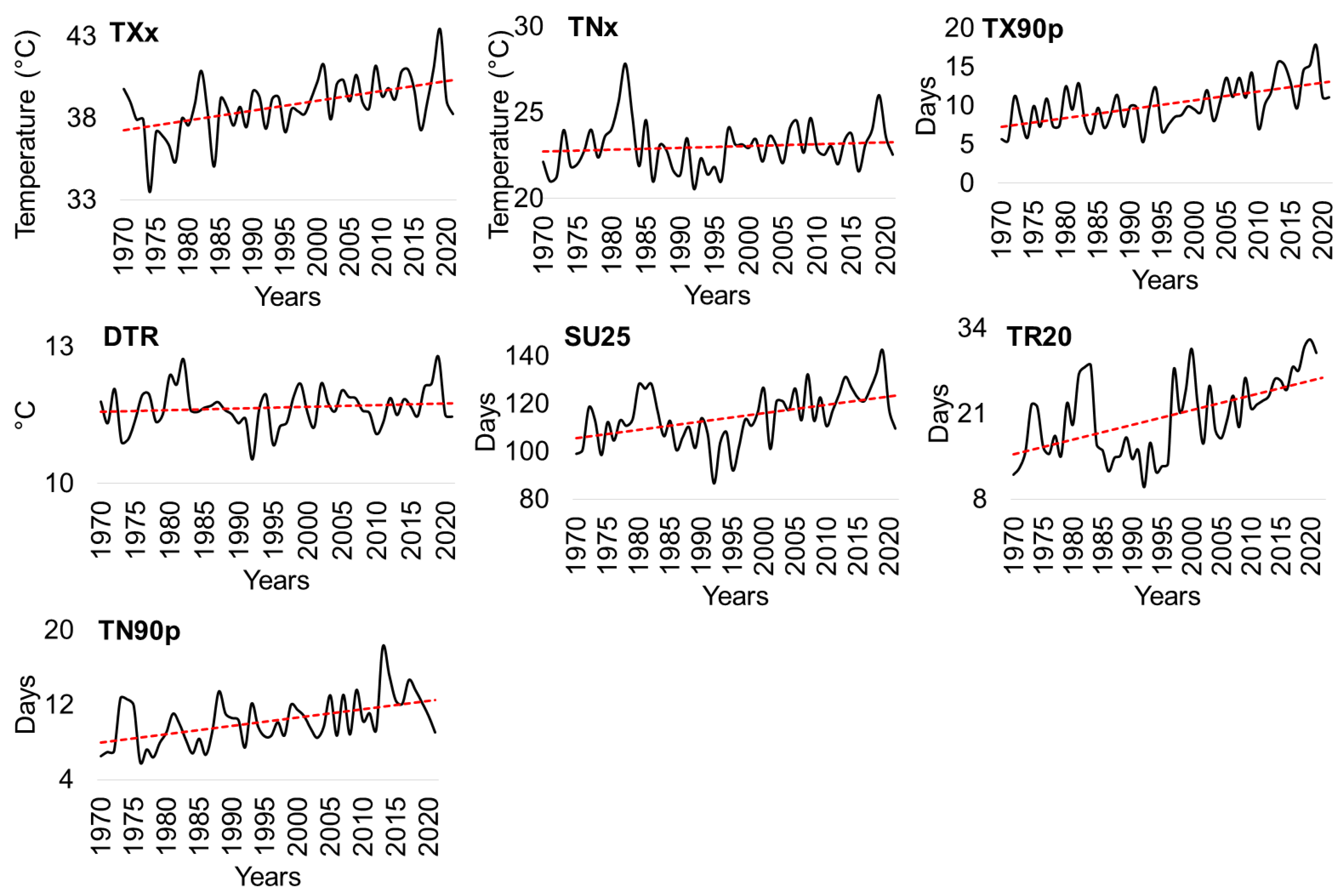
| TXx | Max Tmax | The maximum monthly value of the daily maximum temp | °C |
| TNx | Max Tmin | The maximum monthly value of the daily minimum temp | °C |
| TX90p | Warm days | Percentage of days when TX > 90th percentile | Days |
| DTR | Diurnal temperature range | The monthly mean difference between TX and TN | °C |
| SU25 | Summer days | Annual count when TX (daily maximum) > 25 °C | Days |
| TR20 | Tropical nights | Annual count when TN (daily minimum) > 20 °C | Days |
| TN90p | Warm nights | Percentage of days when TN > 90th percentile | Days |
| Extreme cold temperature events | |||
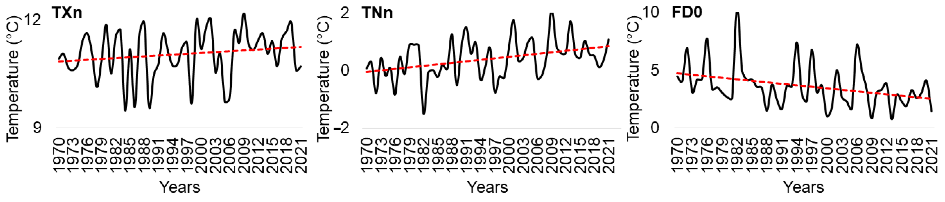
| TXn | Min Tmax | The monthly minimum value of the daily maximum temp | °C |
| TNn | Min Tmin | The monthly minimum value of the daily minimum temp | °C |
| FD0 | Frost days | Annual count when TN (daily minimum) < 0 °C | Days |
| Rainfall events | |||
| PRCPtot | Annual total wet-day precipitation | Annual total PRCP in wet days (RR > 1 mm) | mm |
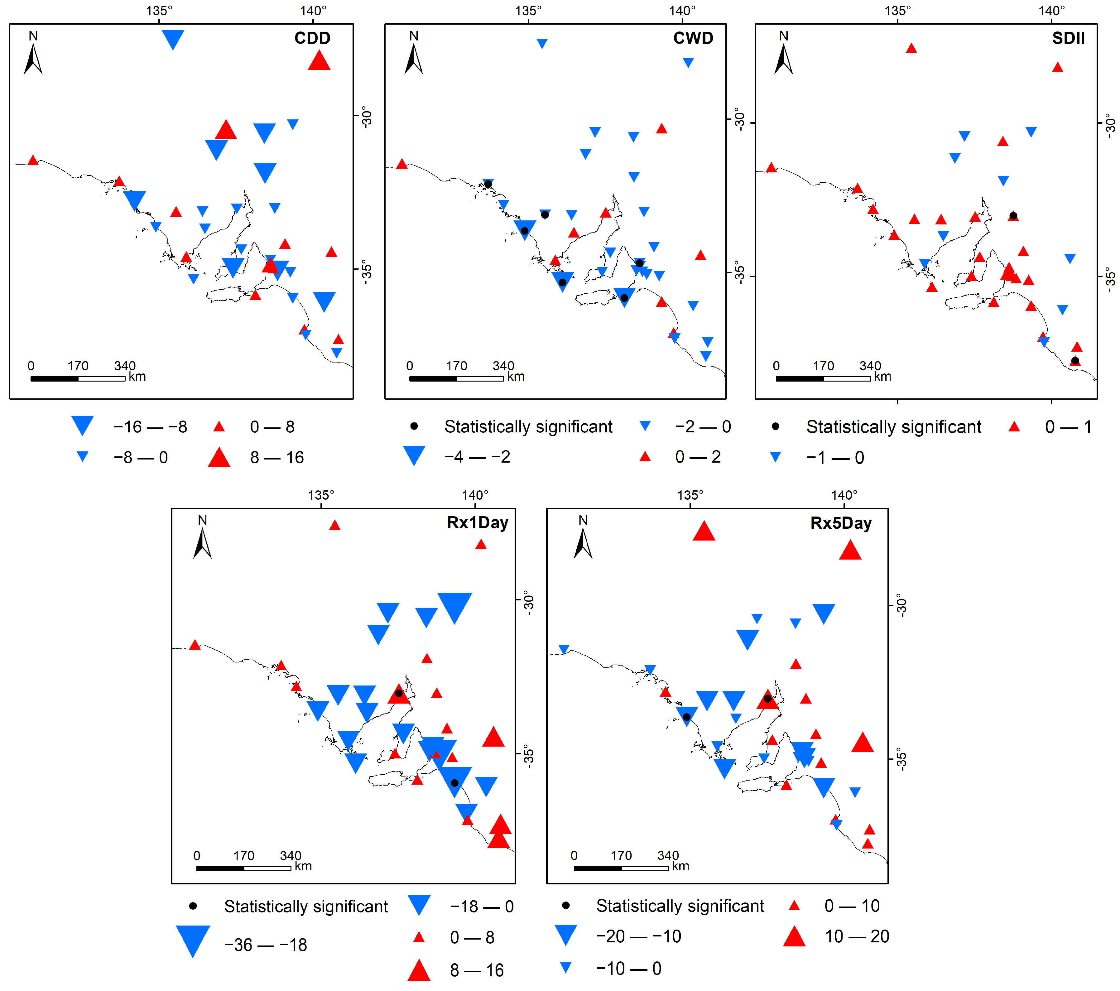
| CDD | Consecutive dry days | Maximum number of successive days with RR < 1 mm | Days |
| CWD | Consecutive wet days | Maximum number of consecutive days with RR > 1 mm | Days |
| SDII | Simple daily intensity index | Annual total precipitation divided by the number of wet days (defined as PRCP ≥ 1 mm) in the year | mm/day |
| RX1day | Max 1-day precipitation amount | Monthly maximum 1-day precipitation | mm |
| Rx5day | Max 5-day precipitation amount | Monthly maximum consecutive 5-day precipitation | mm |
| R10 | Number of heavy precipitation days | Annual count of days when PRCP > 10 mm | Days |
| R20 | Number of very heavy precipitation days | Annual count of days when PRCP > 20 mm | Days |
| R30 | Number of extreme precipitation days | Annual count of days when PRCP > 30 mm | Days |
| R95p | Very wet days | Annual total PRCP when RR > 95th percentile | mm |
| R99p | Extremely wet days | Annual total PRCP when RR > 99th percentile | mm |
3. Results
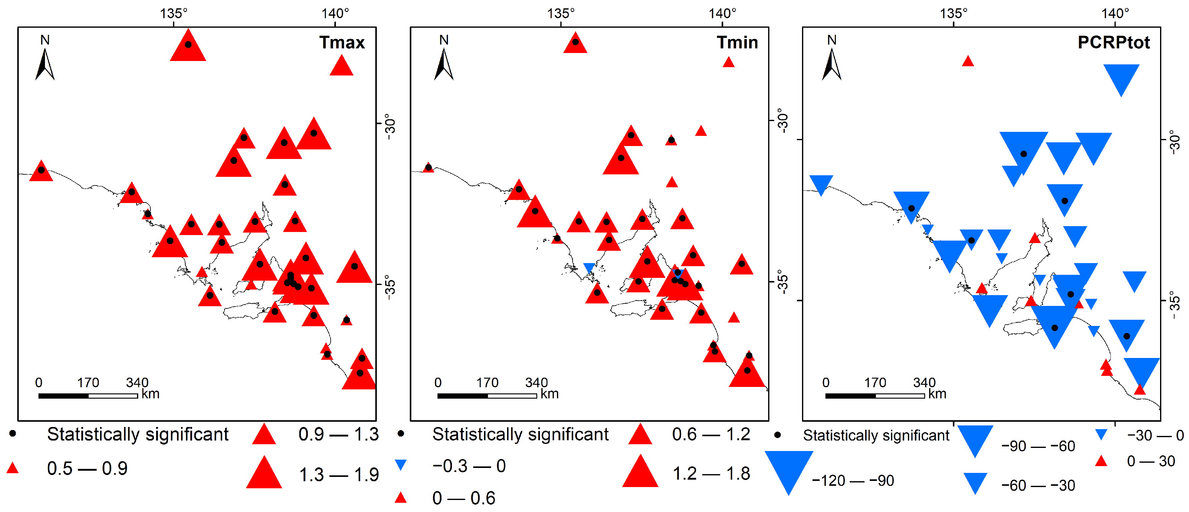
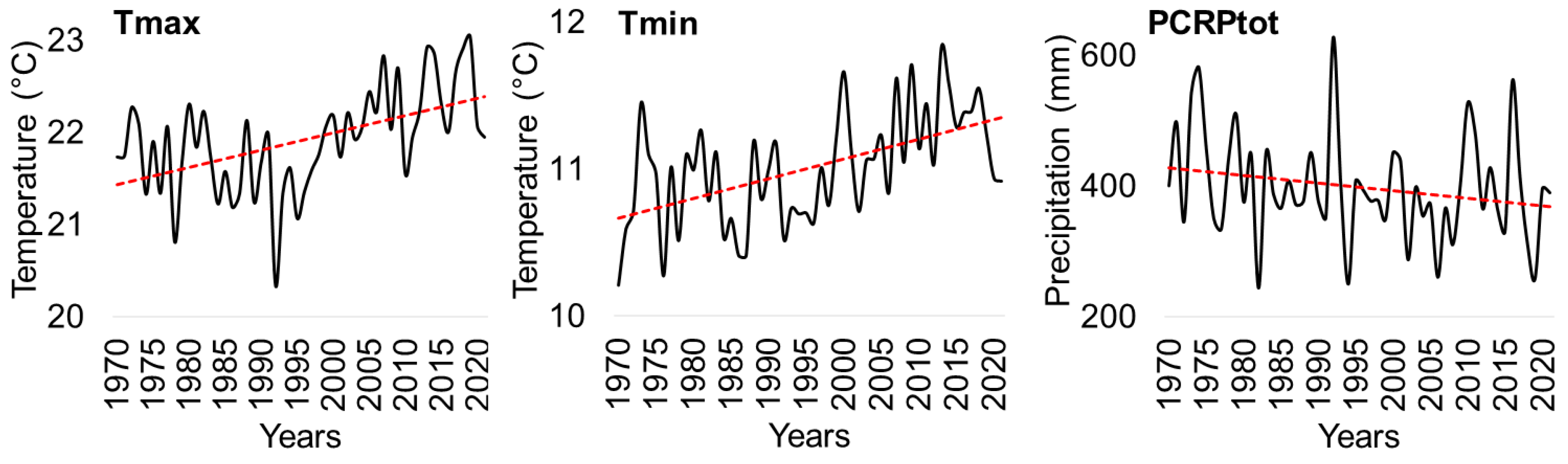
3.1. Temperature and Rainfall Trends
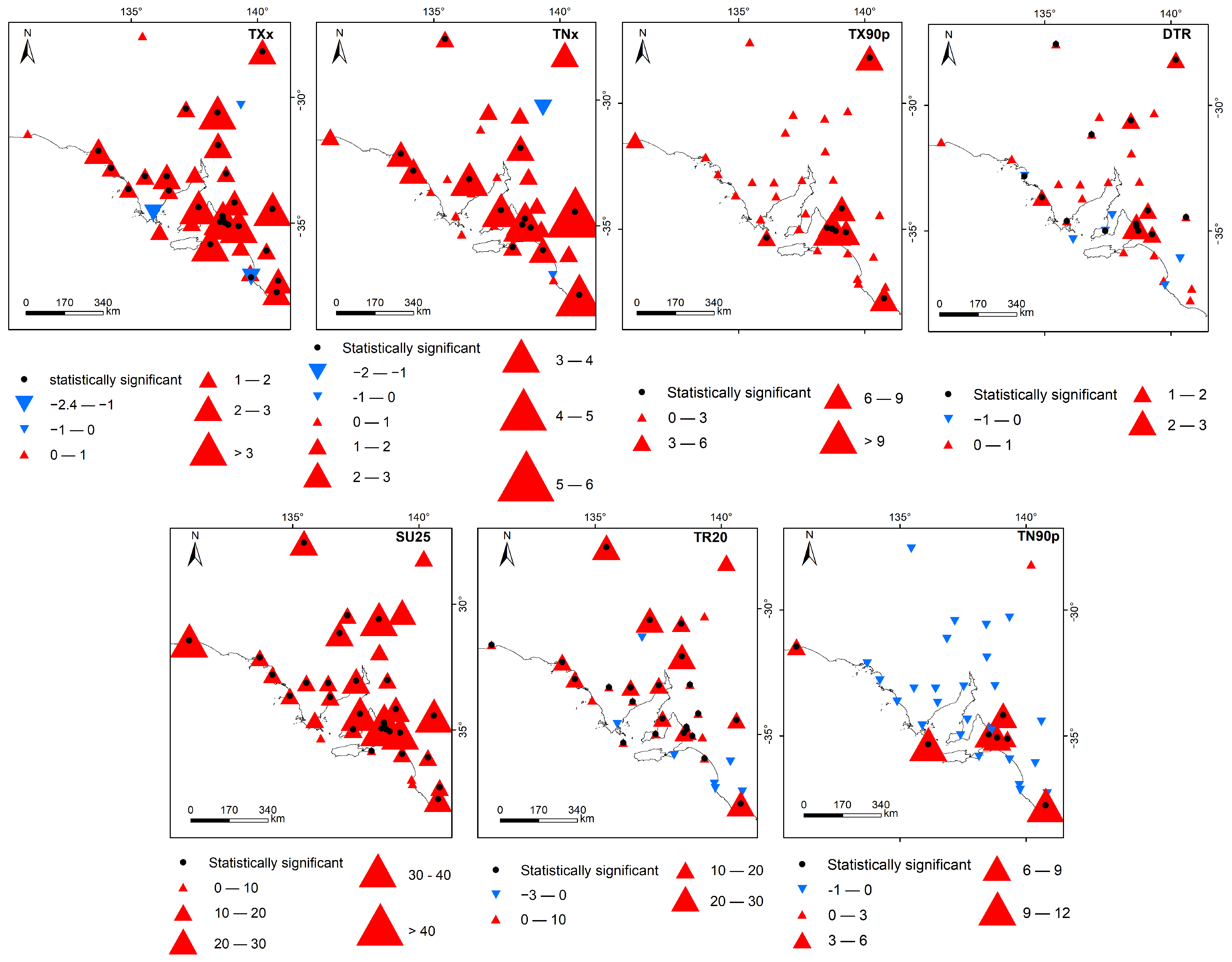
3.2. Extreme Hot Temperature Events
3.3. Extreme Cold Temperature Events
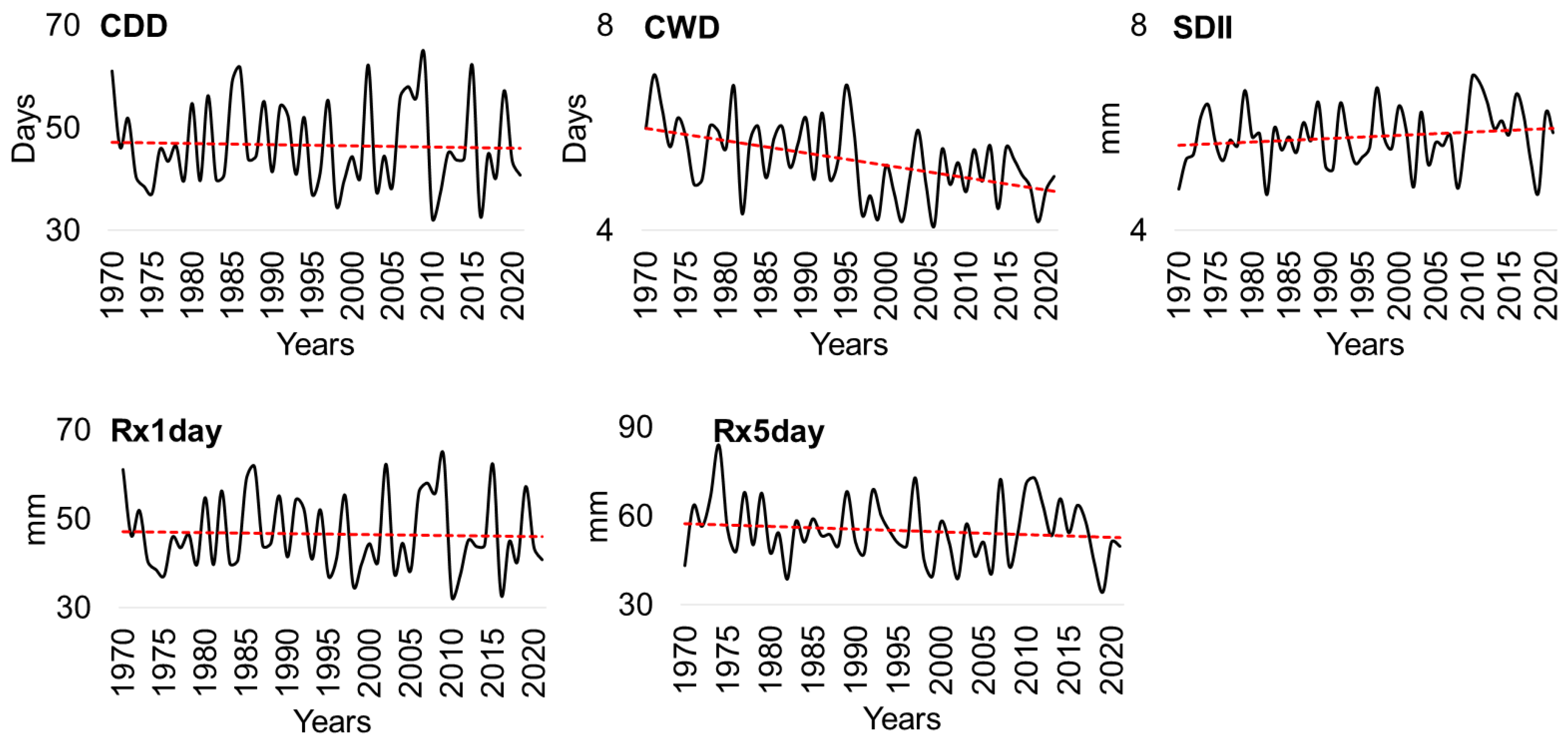
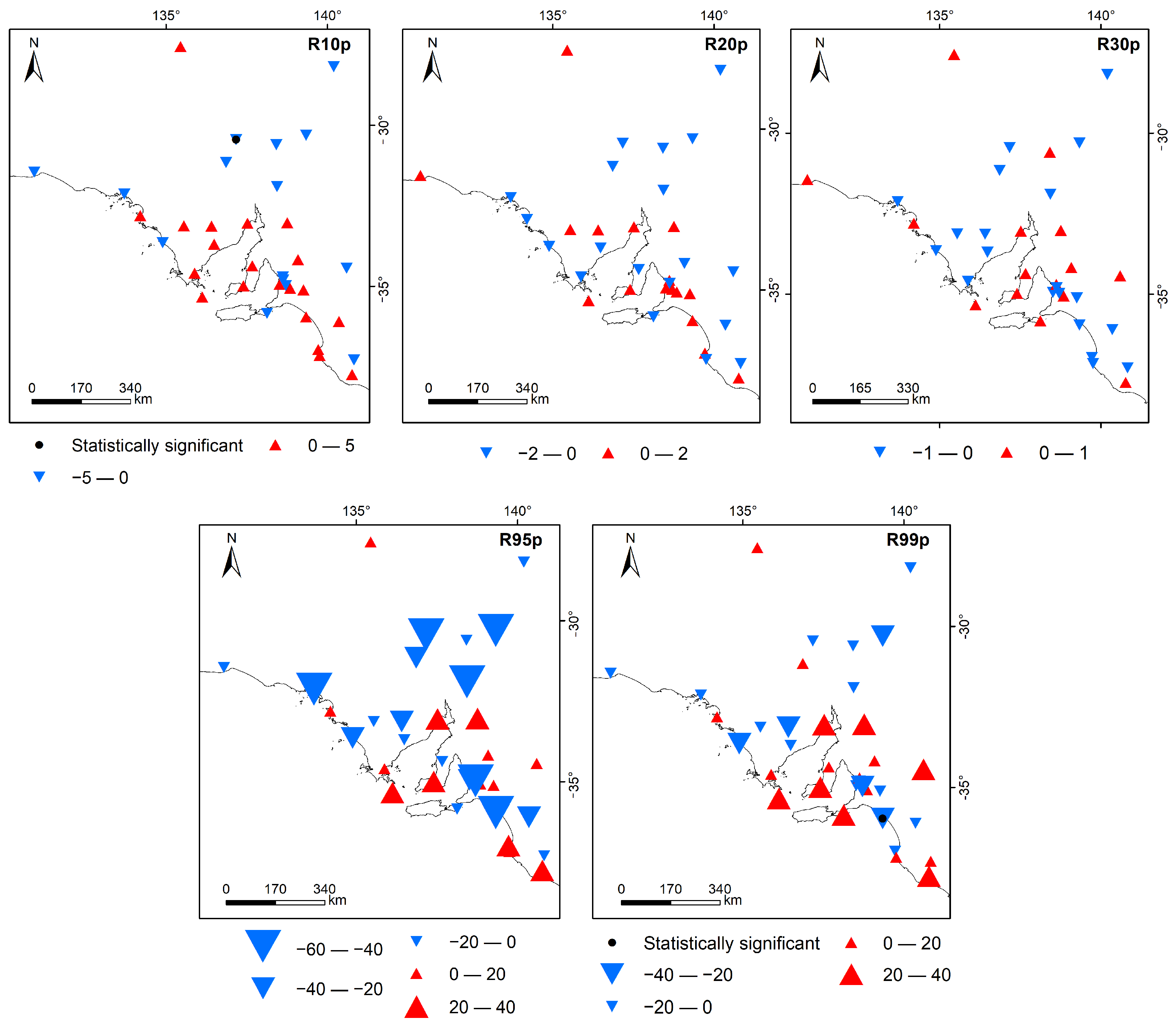
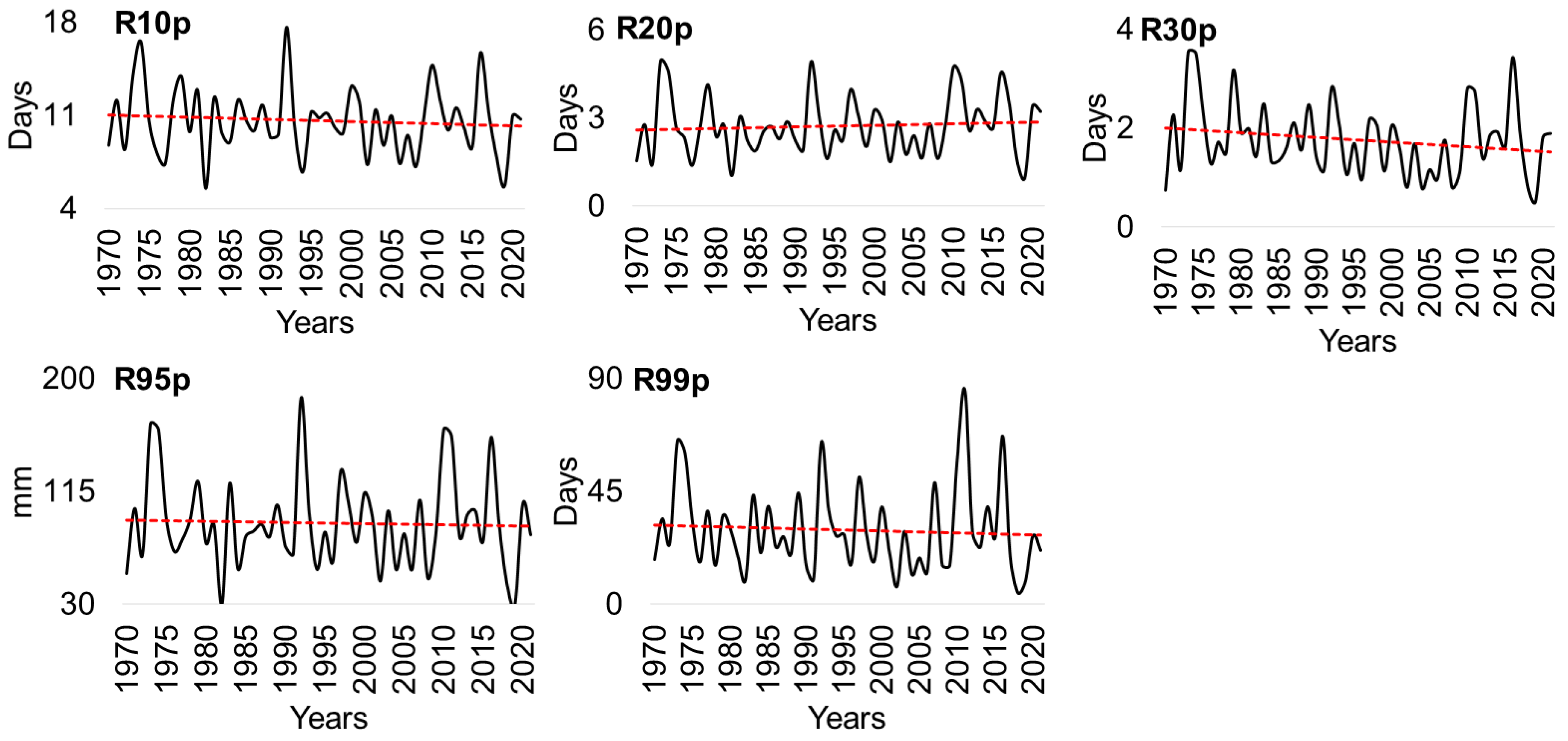
3.4. Daily Rainfall Events
4. Discussion
5. Conclusions
Author Contributions
Funding
Data Availability Statement
Acknowledgments
Conflicts of Interest
References
- Roubille, F.; Matzner-Lober, E.; Aguilhon, S.; Rene, M.; Lecourt, L.; Galinier, M.; Molinari, N. Impact of global warming on weight in patients with heart failure during the 2019 heatwave in France. ESC Heart Fail. 2023, 10, 727–731. [Google Scholar] [CrossRef] [PubMed]
- Zhuang, X.; Hao, Z.; Singh, V.P.; Zhang, Y.; Feng, S.; Xu, Y.; Hao, F. Drought propagation under global warming: Characteristics, approaches, processes, and controlling factors. Sci. Total Environ. 2022, 838, 156021. [Google Scholar] [CrossRef] [PubMed]
- Woolway, R.I.; Albergel, C.; Frölicher, T.L.; Perroud, M. Severe Lake Heatwaves Attributable to Human-Induced Global Warming. Geophys. Res. Lett. 2022, 49, e2021GL097031. [Google Scholar] [CrossRef]
- Evans, G.W. Projected behavioral impacts of global climate change. Annu. Rev. Psychol. 2019, 70, 449–474. [Google Scholar] [CrossRef]
- Li, Z.; Fang, G.; Chen, Y.; Duan, W.; Mukanov, Y. Agricultural water demands in Central Asia under 1.5 °C and 2.0 °C global warming. Agric. Water Manag. 2020, 231, 106020. [Google Scholar] [CrossRef]
- Diffenbaugh, N.S.; Burke, M. Global warming has increased global economic inequality. Proc. Natl. Acad. Sci. USA 2019, 116, 9808–9813. [Google Scholar] [CrossRef]
- Ocko, I.B.; Sun, T.; Shindell, D.; Oppenheimer, M.; Hristov, A.N.; Pacala, S.W.; Hamburg, S.P. Acting rapidly to deploy readily available methane mitigation measures by sector can immediately slow global warming. Environ. Res. Lett. 2021, 16, 054042. [Google Scholar] [CrossRef]
- Stark, C.; Thompson, M.; Andrew, T.; Beasley, G.; Bellamy, O.; Budden, P.; Vause, E. Net Zero: The UK’s Contribution to Stopping Global Warming; Climate Change Committee: London, UK, 2019. [Google Scholar]
- Parker, T.; Gallant, A.; Hobbins, M.; Hoffmann, D. Flash drought in Australia and its relationship to evaporative demand. Environ. Res. Lett. 2021, 16, 064033. [Google Scholar] [CrossRef]
- Phillips, N.; Nogrady, B. The race to decipher how climate change influenced Australia’s record fires. Nature 2020, 577, 610–613. [Google Scholar] [CrossRef]
- Xu, X.; Jia, G.; Zhang, X.; Riley, W.J.; Xue, Y. Climate regime shift and forest loss amplify fire in Amazonian forests. Glob. Chang. Biol. 2020, 26, 5874–5885. [Google Scholar] [CrossRef]
- Abram, N.J.; Henley, B.J.; Sen Gupta, A.; Lippmann, T.J.; Clarke, H.; Dowdy, A.J.; Boer, M.M. Connections of climate change and variability to large and extreme forest fires in southeast Australia. Commun. Earth Environ. 2021, 2, 8. [Google Scholar] [CrossRef]
- McGowan, H.; Theobald, A. Atypical weather patterns cause coral bleaching on the Great Barrier Reef, Australia during the 2021–2022 La Niña. Sci. Rep. 2023, 13, 6397. [Google Scholar] [CrossRef] [PubMed]
- Schneider, M.; Radbone, C.G.; Vasquez, S.A.; Palfy, M.; Stanley, A.K. Population data centre profile: SA NT DataLink (South Australia and Northern Territory). Int. J. Popul. Data Sci. 2019, 4, 1136. [Google Scholar] [CrossRef] [PubMed]
- Rose, T.J.; Parvin, S.; Han, E.; Condon, J.; Flohr, B.M.; Schefe, C.; Kirkegaard, J.A. Prospects for summer cover crops in southern Australian semi-arid cropping systems. Agric. Syst. 2022, 200, 103415. [Google Scholar] [CrossRef]
- Ratnayake, D.C.; Hewa, G.A.; Kemp, D.J. Challenges in quantifying losses in a partly urbanised catchment: A south Australian case study. Water 2022, 14, 1313. [Google Scholar] [CrossRef]
- Wang, B.; Gray, J.M.; Waters, C.M.; Anwar, M.R.; Orgill, S.E.; Cowie, A.L.; Li Liu, D. Modelling and mapping soil organic carbon stocks under future climate change in south-eastern Australia. Geoderma 2022, 405, 115442. [Google Scholar] [CrossRef]
- McGreevy, M.; MacDougall, C.; Fisher, M.; Henley, M.; Baum, F. Expediting a renewable energy transition in a privatised market via public policy: The case of south Australia 2004-18. Energy Policy 2021, 148, 111940. [Google Scholar] [CrossRef]
- Simshauser, P.; Gilmore, J. Climate change policy discontinuity & Australia’s 2016–2021 renewable investment supercycle. Energy Policy 2022, 160, 112648. [Google Scholar]
- Worku, G.; Teferi, E.; Bantider, A.; Dile, Y.T. Observed changes in extremes of daily rainfall and temperature in Jemma sub-basin Upper Blue Nile Basin, Ethiopia. Theor. Appl. Climatol. 2019, 135, 839–854. [Google Scholar] [CrossRef]
- Ferrelli, F.; Brendel, A.S.; Perillo, G.M.E.; Piccolo, M.C. Warming signals emerging from the analysis of daily changes in extreme temperature events over Pampas (Argentina). Environ. Earth Sci. 2021, 80, 422. [Google Scholar] [CrossRef]
- Zhou, H.; Aizen, E.; Aizen, V. Constructing a long-term monthly climate data set in central Asia. Int. J. Climatol. 2018, 38, 1463–1475. [Google Scholar] [CrossRef]
- Zhang, X.; Yang, F. RClimDex (1.1) User Manual. 2013. Available online: http://cccma.Seos.Uvic.Ca/ETCCDI/software.shtml (accessed on 25 October 2022).
- Wang, X.L.; Wen, Q.H.; Wu, Y. Penalized maximal t test for detecting undocumented mean change in climate data series. J. Appl. Meteorol. Climatol. 2007, 46, 916–931. [Google Scholar] [CrossRef]
- Wang, X.L. Penalized maximal F-test for detecting undocumented mean shifts without trend-change. J. Atmos. Ocean. Technol. 2008, 25, 368–384. [Google Scholar] [CrossRef]
- Ruml, M.; Gregorić, E.; Vujadinović, M.; Radovanović, S.; Matović, G.; Vuković, A.; Pocuca, V.; Stojičić, D. Observed changes of temperature extremes in Serbia over the period 1961−2010. Atmos. Res. 2017, 183, 26–41. [Google Scholar] [CrossRef]
- Taylor, M.H.; Losch, M.; Wenzel, M.; Schröter, J. On the sensitivity of eld reconstruction and prediction using empirical orthogonal functions derived from Gappy data. J. Clim. 2013, 26, 9194–9205. [Google Scholar] [CrossRef]
- Kondrashov, D.; Denton, R.; Shprits, Y.Y.; Singer, H.J. Reconstruction of gaps in the past history of solar wind parameters. Geophys. Res. Lett. 2014, 41, 2702–2707. [Google Scholar] [CrossRef]
- Zhang, Q.; Li, J.; Chen, Y.D.; Chen, X. Observed changes of temperature extremes during 1960–2005 in China: Natural or human-induced variations? Theor. Appl. Climatol. 2011, 106, 417–431. [Google Scholar] [CrossRef]
- Ferrelli, F.; Brendel, A.S.; Aliaga, V.S.; Piccolo, M.C.; Perillo, G.M.E. Climate regionalization and trends based on daily temperature and precipitation extremes in the south of the Pampas (Argentina). Cuad. Investig. Geogr. 2019, 45, 393–416. [Google Scholar] [CrossRef]
- Chen, A.; He, X.; Guan, H.; Cai, Y. Trends and periodicity of daily temperature and precipitation extremes during 1960–2013 in Hunan Province, central south China. Theor. Appl. Climatol. 2017, 132, 71–88. [Google Scholar] [CrossRef]
- Mann, H.B. Non-parametric tests against trend. Econométrica 1945, 13, 245–259. [Google Scholar] [CrossRef]
- Kendall, M.R. Rank Correlation Methods, 4th ed.Chareles Griffin: London, UK, 1955. [Google Scholar]
- Pohlert, T. Non-parametric trend tests and change-point detection. CC BY-ND 2016, 4, 1–18. [Google Scholar]
- Hamed, K.H. Trend detection in hydrologic data: The Mann–Kendall trend test under the scaling hypothesis. J. Hydrol. 2008, 349, 350–363. [Google Scholar] [CrossRef]
- Alhaji, U.U.; Yusuf, A.S.; Edet, C.O.; Oche, C.O.; Agbo, E.P. Trend analysis of temperature in Gombe state using mann kendall trend test. J. Sci. Res. Rep. 2018, 20, 1–9. [Google Scholar] [CrossRef]
- Peterson, T.; Folland, C.; Gruza, G.; Hogg, W.; Mokssit, A.; Plummer, N. Report on the Activities of the Working Group on Climate Change Detection and Related Rapporteurs; World Meteorological Organization: Geneva, Switzerland, 2001; p. 146. [Google Scholar]
- Sun, W.; Mu, X.; Song, X.; Wu, D.; Cheng, A.; Qiu, B. Changes in extreme temperature and precipitation events in the Loess Plateau (China) during 1960–2013 under global warming. Atmos. Res. Lett. 2016, 168, 33–48. [Google Scholar] [CrossRef]
- Ferrelli, F. Remote Sensing applications for effective fire disaster management plans: A review. Inf. Syst. Smart City 2023, 3, 1–17. [Google Scholar] [CrossRef]
- Ferrelli, F.; Brendel, A.S.; Piccolo, M.C.; Perillo, G.M.E. Tendencia actual y futura de la precipitación en el sur de la Región Pampeana (Argentina). Investig. Geogr. 2020, 102. [Google Scholar] [CrossRef]
- Ferrelli, F.; Brendel, A.; Piccolo, M.C.; Perillo, G.M.E. Evaluación de la tendencia de la precipitación en la región pampeana (Argentina) durante el período 1960–2018. RA’EGA 2021, 51, 41–57. [Google Scholar] [CrossRef]
- Gérard, M.; Vanderplanck, M.; Wood, T.; Michez, D. Global warming and plant–pollinator mismatches. Emerg. Top. Life Sci. 2020, 4, 77–86. [Google Scholar]
- Deng, K.; Azorin-Molina, C.; Yang, S.; Hu, C.; Zhang, G.; Minola, L.; Chen, D. Changes of Southern Hemisphere westerlies in the future warming climate. Atmos. Res. 2022, 270, 106040. [Google Scholar] [CrossRef]
- Abbass, K.; Qasim, M.Z.; Song, H.; Murshed, M.; Mahmood, H.; Younis, I. A review of the global climate change impacts, adaptation, and sustainable mitigation measures. Environ. Sci. Pollut. Res. 2022, 29, 42539–42559. [Google Scholar] [CrossRef]
- Zandalinas, S.I.; Fritschi, F.B.; Mittler, R. Global warming, climate change, and environmental pollution: Recipe for a multifactorial stress combination disaster. Trends Plant Sci. 2021, 26, 588–599. [Google Scholar] [CrossRef] [PubMed]
- Fernández-Long, M.E.; Müller, G.V.; Beltrán-Przekurat, A.; Scarpati, O.E. Long-term and recent changes in temperature-based agroclimatic indices in Argentina. Int. J. Climatol. 2013, 33, 1673–1686. [Google Scholar] [CrossRef]
- Sun, W.; Song, X.; Mu, X.; Gao, P.; Wang, F.; Zhao, G. Spatiotemporal vegetation cover variations associated with climate change and ecological restoration in the Loess Plateau. Agric. Meteorol. 2015, 209, 87–99. [Google Scholar] [CrossRef]
- Zilio, M.I.; Alfonso, M.B.; Ferrelli, F.; Perillo, G.M.E.; Piccolo, M.C. Ecosystem services provision, tourism and climate variability in shallow lakes: The case of La Salada, Buenos Aires, Argentina. Tour. Manag. 2017, 62, 208–217. [Google Scholar] [CrossRef]
- Thakuri, S.; Dahal, S.; Shrestha, D.; Guyennon, N.; Romano, E.; Colombo, N.; Salerno, F. Elevation-dependent warming of maximum air temperature in Nepal during 1976–2015. Atmos. Res. Lett. 2019, 228, 261–269. [Google Scholar] [CrossRef]
- Lim, S.S.; Vos, T.; Flaxman, A.D.; Danaei, G.; Shibuya, K.; Adair-Rohani, H.; Aryee, M. A comparative risk assessment of burden of disease and injury attributable to 67 risk factors and risk factor clusters in 21 regions, 1990–2010: A systematic analysis for the Global Burden of Disease Study 2010. Lancet 2012, 380, 2224–2260. [Google Scholar] [CrossRef] [PubMed]
- Gallant, A.J.; Karoly, D.J. A combined climate extremes index for the Australian region. J. Clim. 2010, 23, 6153–6165. [Google Scholar] [CrossRef]
- Alexander, L.V.; Arblaster, J.M. Historical and projected trends in temperature and precipitation extremes in Australia in observations and CMIP5. Weather. Clim. Extrem. 2017, 15, 34–56. [Google Scholar] [CrossRef]
- Grose, M.R.; Narsey, S.; Delage, F.P.; Dowdy, A.J.; Bador, M.; Boschat, G.; Power, S. Insights from CMIP6 for Australia’s future climate. Earth’s Future 2020, 8, e2019EF001469. [Google Scholar] [CrossRef]
- Sharma, A.; Wasko, C.; Lettenmaier, D.P. If precipitation extremes are increasing, why aren’t foods? Water Resour. Res. 2018, 54, 8545–8551. [Google Scholar] [CrossRef]
- Blöschl, G.; Hall, J.; Parajka, J.; Perdigão, R.A.; Merz, B.; Arheimer, B.; Živković, N. Changing climate shifts timing of European floods. Science 2017, 357, 588–590. [Google Scholar] [CrossRef] [PubMed]
- Willoughby, N.; Thompson, D.; Royal, M.; Miles, M. South Australian Land Cover Layers: An Introduction and Summary Statistics; Department for Environment and Water: Adelaide, Australia, 2018. [Google Scholar]
- Climate Council of Australia. Australia’s Rising Greenhouse Gas Emissions; Climate Council: Potts Point, Australia, 2018. [Google Scholar]
- Panchasara, H.; Samrat, N.H.; Islam, N. Greenhouse gas emissions trends and mitigation measures in Australian agriculture sector—A review. Agriculture 2021, 11, 85. [Google Scholar] [CrossRef]
- Trenberth, K.E. Understanding climate change through Earth’s energy flows. J. R. Soc. N. Z. 2020, 50, 331–347. [Google Scholar] [CrossRef]
- Islam, N.; Ray, B.; Pasandideh, F. IoT based smart farming: Are the LPWAN technologies suitable for remote communication? In Proceedings of the 2020 IEEE International Conference on Smart Internet of Things (SmartIoT), Beijing, China, 14–16 August 2020; pp. 270–276. [Google Scholar]
- Alam, M.; Alam, M.S.; Roman, M.; Tufail, M.; Khan, M.U.; Khan, M.T. Real-time machine-learning based crop/weed detection and classification for variable-rate spraying in precision agriculture. In Proceedings of the 2020 7th International Conference on Electrical and Electronics Engineering (ICEEE), Antalya, Turkey, 14–16 April 2020; pp. 273–280. [Google Scholar]
- Saravanan, K.; Saraniya, S. Cloud IOT based novel livestock monitoring and identification system using UID. Sens. Rev. 2017, 38, 21–33. [Google Scholar]
- Xu, M.J.; Plonowska, K.A.; Gurman, Z.R.; Humphrey, A.K.; Ha, P.K.; Wang, S.J.; El-Sayed, I.H.; Heaton, C.M.; George, J.R.; Yom, S.S.; et al. Treatment modality impact on quality of life for human papillomavirus– associated oropharynx cancer. Laryngoscope 2020, 130, E48–E56. [Google Scholar] [CrossRef]
- Tierney, J.; Smerdon, J.; Anchukaitis, K.; Seager, R. Multidecadal variability in East African hydroclimate controlled by the Indian Ocean. Nature 2013, 493, 389–392. [Google Scholar] [CrossRef]
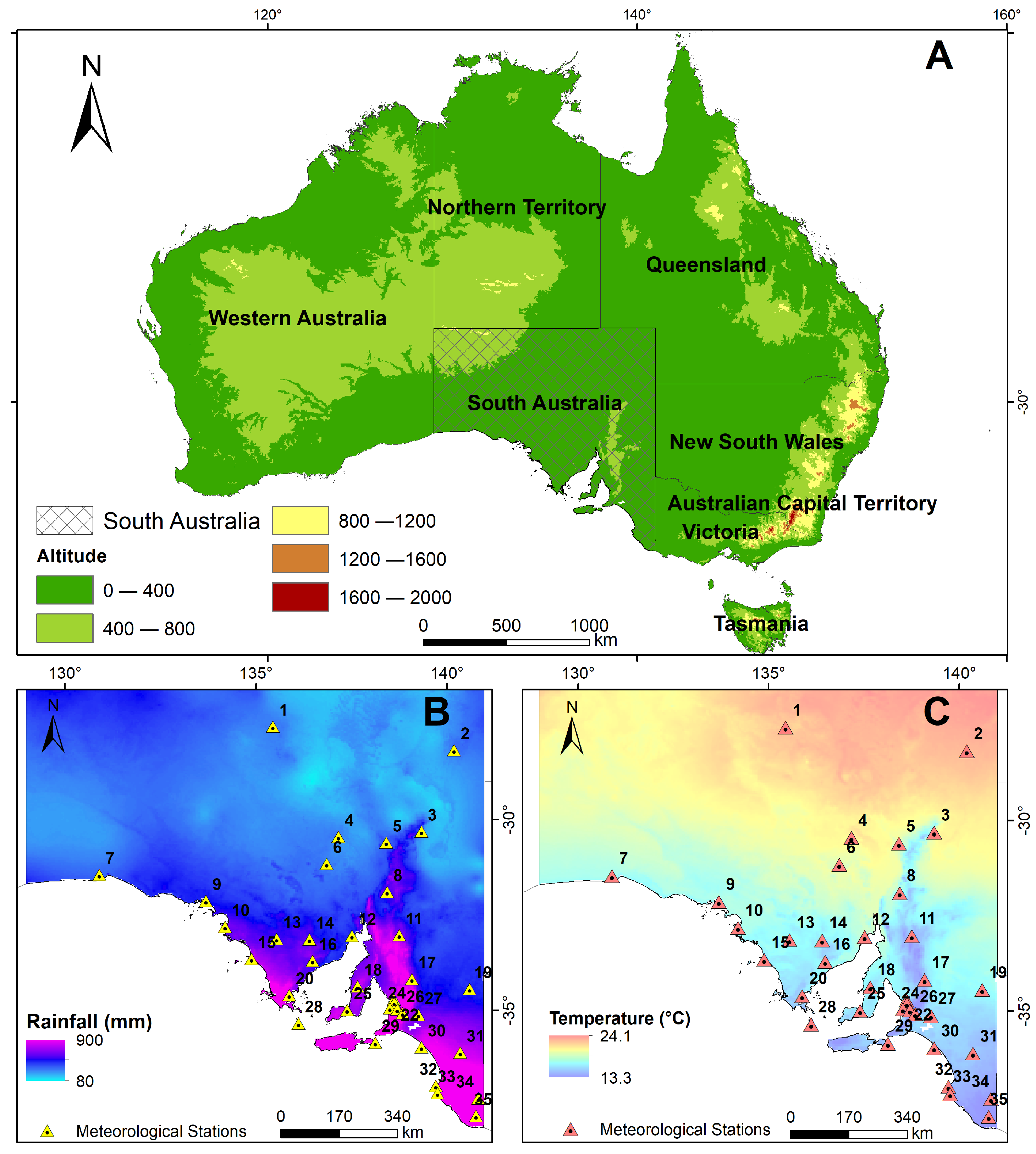


| ID | Weather Station | Lat | Long | Altitude (m) | Period | Tmax (°C) | Tmin (°C) | Pp (mm) |
|---|---|---|---|---|---|---|---|---|
| 1 | Woomera Aerodrome | −31.16 | 136.86 | 167 | 1949–2021 | 25.8 ± 6.5 | 12.7 ± 5.1 | 179.8 ± 81.4 |
| 2 | Andamooka | −30.45 | 137.17 | 76 | 1965–2021 | 26.1 ± 6.6 | 13.8 ± 5.7 | 181.9 ± 100.9 |
| 3 | Oodnadatta Airport | −27.56 | 135.45 | 117 | 1939–2021 | 29.1 ± 6.7 | 12.7 ± 5.3 | 168.8 ± 99.7 |
| 4 | Arkaroola | −30.31 | 139.34 | 318 | 1938–2021 | 25.7 ± 6.4 | 11.5 ± 6.1 | 246.8 ± 160.9 |
| 5 | Leigh Creek Airport | −30.6 | 138.42 | 259 | 1982–2021 | 26.3 ± 6.9 | 12.8 ± 5.9 | 207.8 ± 102.2 |
| 6 | Moomba Airport | −28.18 | 140.2 | 38 | 1995–2021 | 29.6 ± 6.8 | 15.5 ± 6.7 | 161.7 ± 126.3 |
| 7 | Ceduna Amo | −32.13 | 133.7 | 15 | 1939–2021 | 23.5 ± 4.05 | 10.4 ± 3.5 | 293.4 ± 84.4 |
| 8 | Cleve | −33.7 | 136.49 | 193 | 1986–2021 | 22.5 ± 4.7 | 11.6 ± 3.3 | 399.1 ± 97.2 |
| 9 | Kimba | −33.14 | 136.41 | 280 | 1920–2021 | 23.8 ± 5.9 | 10.4 ± 4.1 | 341.9 ± 106.1 |
| 10 | Kyancutta | −33.13 | 135.55 | 59 | 1930–2021 | 25.2 ± 5.8 | 9.3 ± 3.6 | 310.6 ± 79.09 |
| 11 | Elliston | −33.65 | 134.89 | 7 | 1882–2021 | 21.5 ± 3.5 | 11.8 ± 2.9 | 422.6 ± 100.1 |
| 12 | Streaky Bay | −32.81 | 134.2 | 45 | 1865–2021 | 23.3 ± 4.61 | 13.2 ± 2.9 | 371.8 ± 97.6 |
| 13 | Nullarbor | −31.45 | 130.9 | 64 | 1888–2021 | 23.8 ± 3.5 | 10.8 ± 3.94 | 186.9 ± 147.8 |
| 14 | Neptune Island | −35.34 | 136.12 | 32 | 1957–2021 | 18.6 ± 2.58 | 13.8 ± 1.9 | 403.2 ± 143.9 |
| 15 | Whyalla Aero | −33.05 | 137.52 | 9 | 1945–2021 | 23.7 ± 4.8 | 11.5 ± 4.7 | 243.7 ± 96.1 |
| 16 | North Shields (Port Lincoln Aws) | −34.6 | 135.88 | 9 | 1992–2021 | 22.2 ± 3.7 | 11.3 ± 3.3 | 379.6 ± 92.8 |
| 17 | Hawker | −31.9 | 138.44 | 340 | 1882–2021 | 24.5 ± 6.7 | 10.8 ± 5.4 | 300.4 ± 121.1 |
| 18 | Adelaide Airport | −34.95 | 138.52 | 2 | 1955–2021 | 21.5 ± 4.7 | 11.5 ± 3.4 | 438.4 ± 102.8 |
| 19 | Adelaide West Terrace | −34.93 | 138.58 | 29 | 1839–2021 | 21.8 ± 5.05 | 12.02 ± 3.38 | 521.3 ± 115.7 |
| 20 | Cape Jaffa | −36.97 | 139.72 | 17 | 1991–2021 | 19.2 ± 3.9 | 12.4 ± 2.3 | 488 ± 111.8 |
| 21 | Cape Willoughby | −35.84 | 138.13 | 55 | 1881–2021 | 18.1 ± 2.8 | 12.8 ± 2.4 | 528.6 ± 129.8 |
| 22 | Coonawarra | −37.29 | 140.83 | 57 | 1985–2021 | 20.4 ± 5.06 | 8.1 ± 2.4 | 563.3 ± 112.6 |
| 23 | Edinburgh RAAF | −34.71 | 138.62 | 17 | 1972–2021 | 22.6 ± 5.46 | 11.1 ± 3.9 | 417.2 ± 112.9 |
| 24 | Eudunda | −34.18 | 139.09 | 420 | 1882–2021 | 21.1 ± 6.03 | 9.2 ± 3.4 | 445.1± 120.7 |
| 25 | Keith | −36.1 | 140.36 | 29 | 1906–2021 | 22.3 ± 5.58 | 9.2 ± 2.9 | 453.9± 101.8 |
| 26 | Loxton Research Centre | −34.44 | 140.6 | 30 | 1984–2021 | 23.9 ± 5.9 | 9.08 ± 4.01 | 260 ± 77.6 |
| 27 | Maitland | −34.37 | 137.67 | 185 | 1879–2021 | 21.7 ± 5.4 | 11.24 ± 4.02 | 487.8 ± 131.4 |
| 28 | Maningie | −35.96 | 139.34 | 3 | 1864–2021 | 21.03 ± 4.1 | 10.41 ± 2.7 | 441.4 ± 145.1 |
| 29 | Mount Barker | −35.07 | 138.85 | 359 | 1861–2021 | 20.2 ± 5.2 | 8.2 ± 2.7 | 748.5 ± 193.2 |
| 30 | Mount Gambier Aero | −37.75 | 140.77 | 63 | 1941–2021 | 19.02 ± 4.4 | 8.2 ± 2.3 | 714.6 ± 123.5 |
| 31 | Mount Lofty | −34.98 | 138.71 | 685 | 1985–2021 | 22.9 ± 5.1 | 8.7 ± 2.8 | 791.4 ± 123.6 |
| 32 | Murray Bridge | −35.12 | 139.26 | 33 | 1885–2021 | 15.9 ± 4.8 | 9.8 ± 3.5 | 714.6 ± 205.2 |
| 33 | Parafield Airport | −34.8 | 138.63 | 10 | 1929–2021 | 22.5 ± 5.4 | 10.8 ± 3.8 | 431.2 ± 103.6 |
| 34 | Price | −34.3 | 138 | 2 | 1944–2021 | 22.8 ± 4.6 | 11.2 ± 3.7 | 322.8 ± 88.9 |
| 35 | Robe | −37.16 | 139.76 | 3 | 1860–2021 | 18.1 ± 3.3 | 10.9 ± 2.01 | 621.5 ± 134.8 |
| 36 | Warooka | −34.99 | 137.4 | 53 | 1861–2021 | 21.2 ± 4.5 | 11.6 ± 3.07 | 438.7 ± 97.8 |
| 37 | Yongala | −33.03 | 138.76 | 521 | 1881–2021 | 22.01 ± 6.6 | 7.4 ± 4.3 | 345.4 ± 125 |
Disclaimer/Publisher’s Note: The statements, opinions and data contained in all publications are solely those of the individual author(s) and contributor(s) and not of MDPI and/or the editor(s). MDPI and/or the editor(s) disclaim responsibility for any injury to people or property resulting from any ideas, methods, instructions or products referred to in the content. |
© 2024 by the authors. Licensee MDPI, Basel, Switzerland. This article is an open access article distributed under the terms and conditions of the Creative Commons Attribution (CC BY) license (https://creativecommons.org/licenses/by/4.0/).
Share and Cite
Ferrelli, F.; Pontrelli Albisetti, M.; Brendel, A.S.; Casoni, A.I.; Hesp, P.A. Appraisal of Daily Temperature and Rainfall Events in the Context of Global Warming in South Australia. Water 2024, 16, 351. https://doi.org/10.3390/w16020351
Ferrelli F, Pontrelli Albisetti M, Brendel AS, Casoni AI, Hesp PA. Appraisal of Daily Temperature and Rainfall Events in the Context of Global Warming in South Australia. Water. 2024; 16(2):351. https://doi.org/10.3390/w16020351
Chicago/Turabian StyleFerrelli, Federico, Melisa Pontrelli Albisetti, Andrea Soledad Brendel, Andrés Iván Casoni, and Patrick Alan Hesp. 2024. "Appraisal of Daily Temperature and Rainfall Events in the Context of Global Warming in South Australia" Water 16, no. 2: 351. https://doi.org/10.3390/w16020351
APA StyleFerrelli, F., Pontrelli Albisetti, M., Brendel, A. S., Casoni, A. I., & Hesp, P. A. (2024). Appraisal of Daily Temperature and Rainfall Events in the Context of Global Warming in South Australia. Water, 16(2), 351. https://doi.org/10.3390/w16020351