
Towards Non-Region Specific Large-Scale Inundation Modelling with Machine Learning Methods


Abstract
1. Introduction
Prior Work
2. Materials and Methods
2.1. Dataset
2.2. Preprocessing
3. Machine Learning Method
- (a)
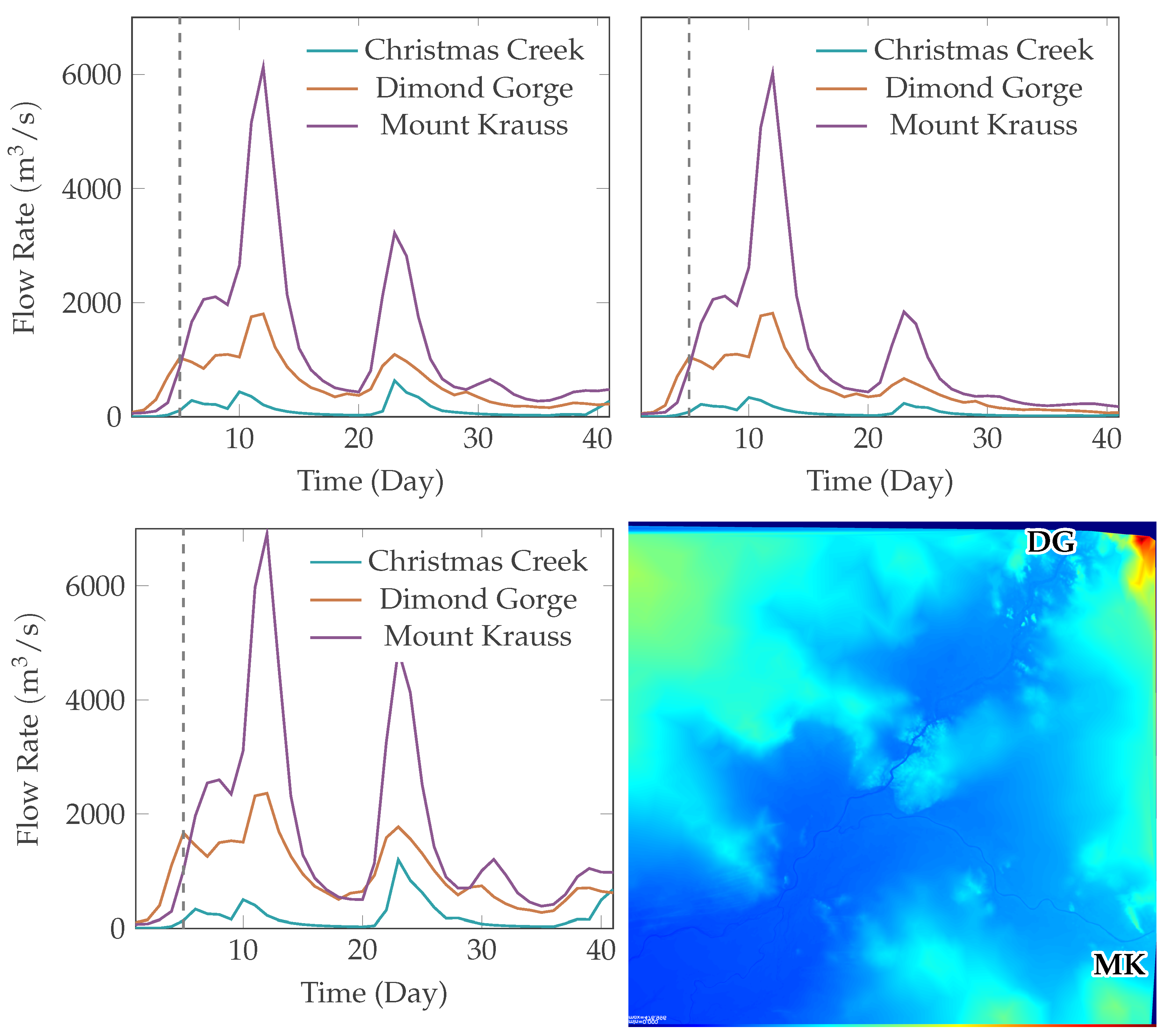
- Inflow Model: predicts the change in water height for local regions containing a single inflow boundary with known inflow or discharge rate. In our dataset there are 3 inflow boundaries: Christmas Creek, Dimond Gorge and Mount Krauss. Each inflow boundary has an inflow rate defined over the modelling time period.
- (b)
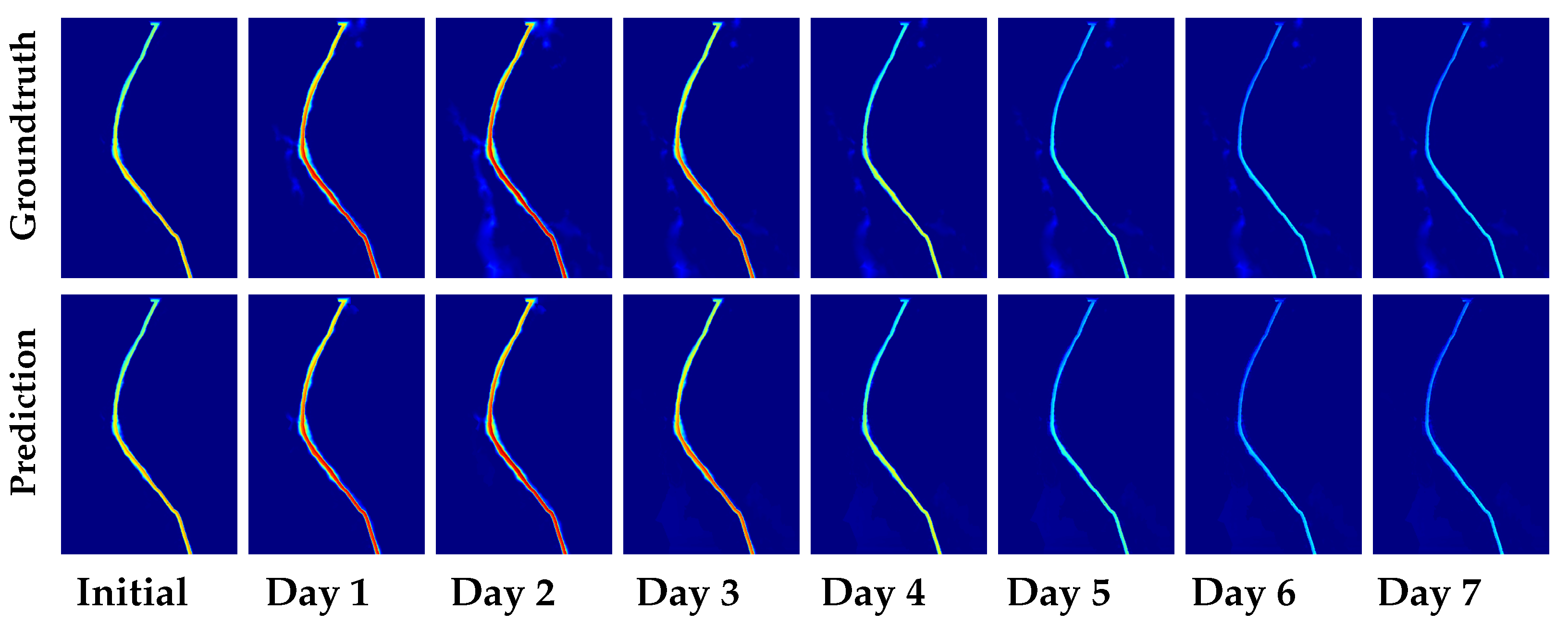
- Interior Model: predicts the change in water height for all local regions not predicted by the Inflow model. This model is responsible for propagating the water generated by the Inflow model through the rest of the river system.
3.1. Input Transforms
3.2. Water Height Regression
3.3. Network Topology
3.4. Model Training
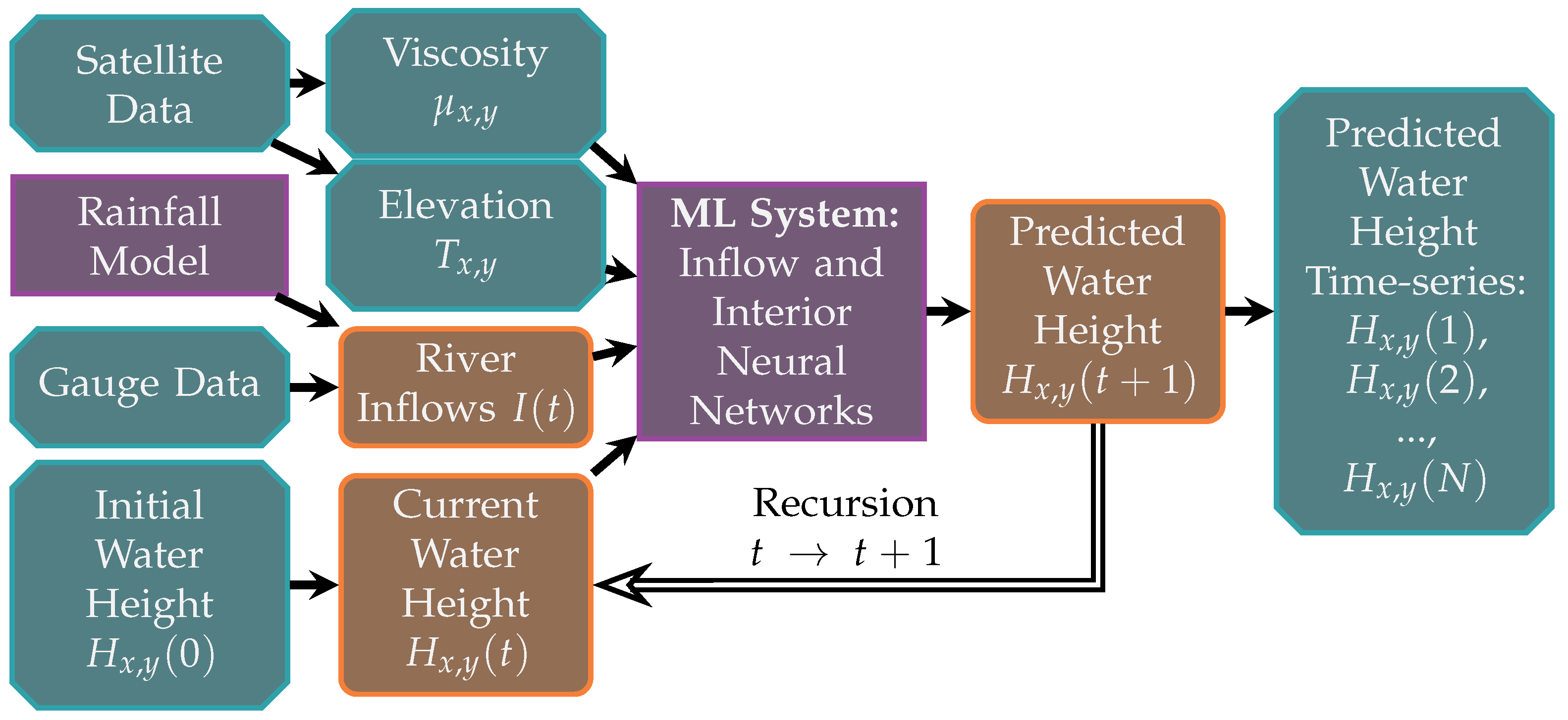
3.5. Inference Method
- Extract the current water height, elevation, roughness and driving inflow data from the three grid cells which contain the driving inflows.
- Apply the Inflow model to these regions to predict a set of local water heights for the next timestep
- By observing the current global water height identify all grid cells which contain any water. To this set of regions add the surrounding regions to form the water cells. For each water cell extract the associated local region from the elevation, roughness, water height, flow and driving inflow data.
- Apply the Interior model to the extracted water regions to predict a set of local water heights
- Combine local outputs of both Inflow and Interior models and to reconstruct the global water height and change in water height . Only the central values from the local ML model predictions is used.
- Repeat steps 1–5 until desired time has elapsed
4. Results
4.1. Inflow Model
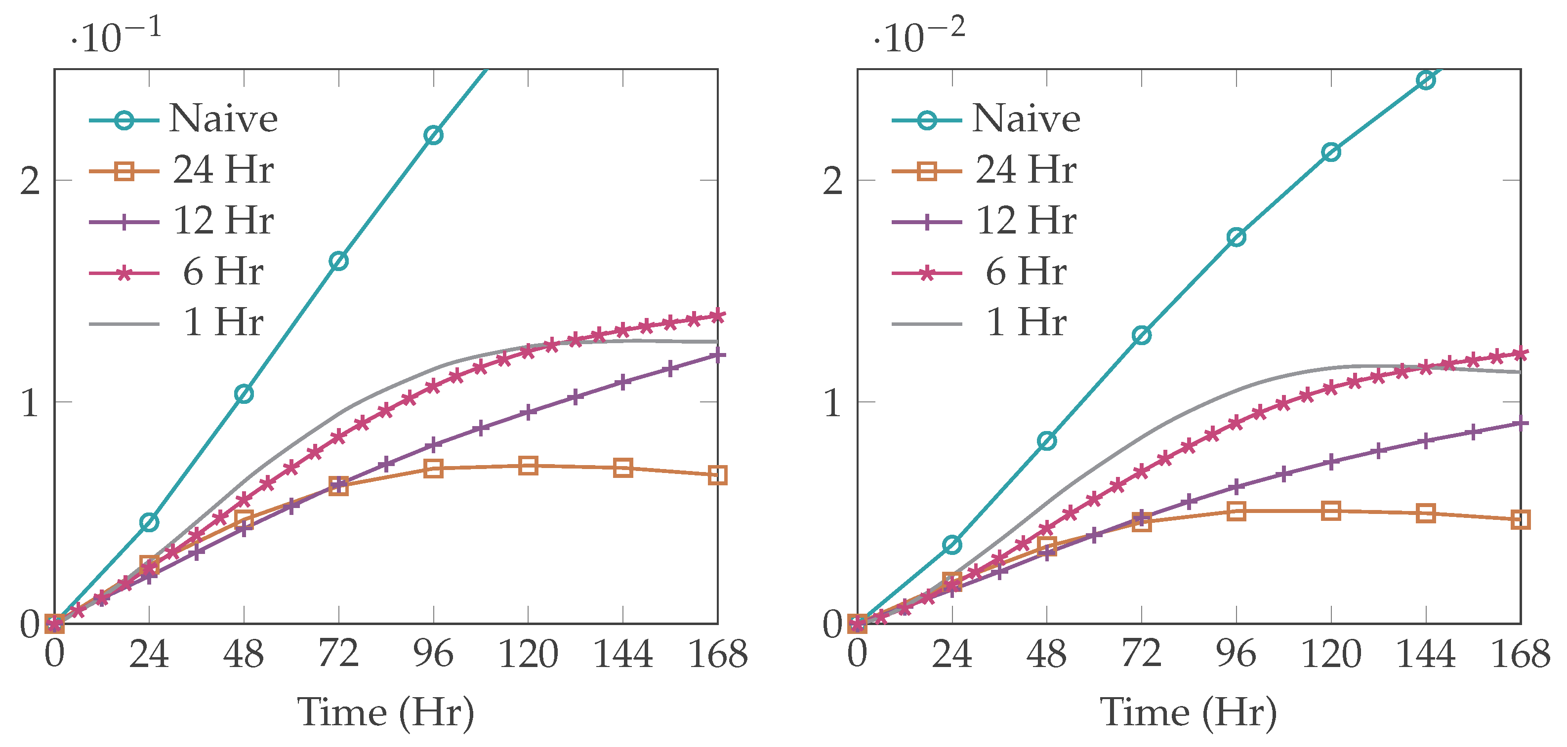
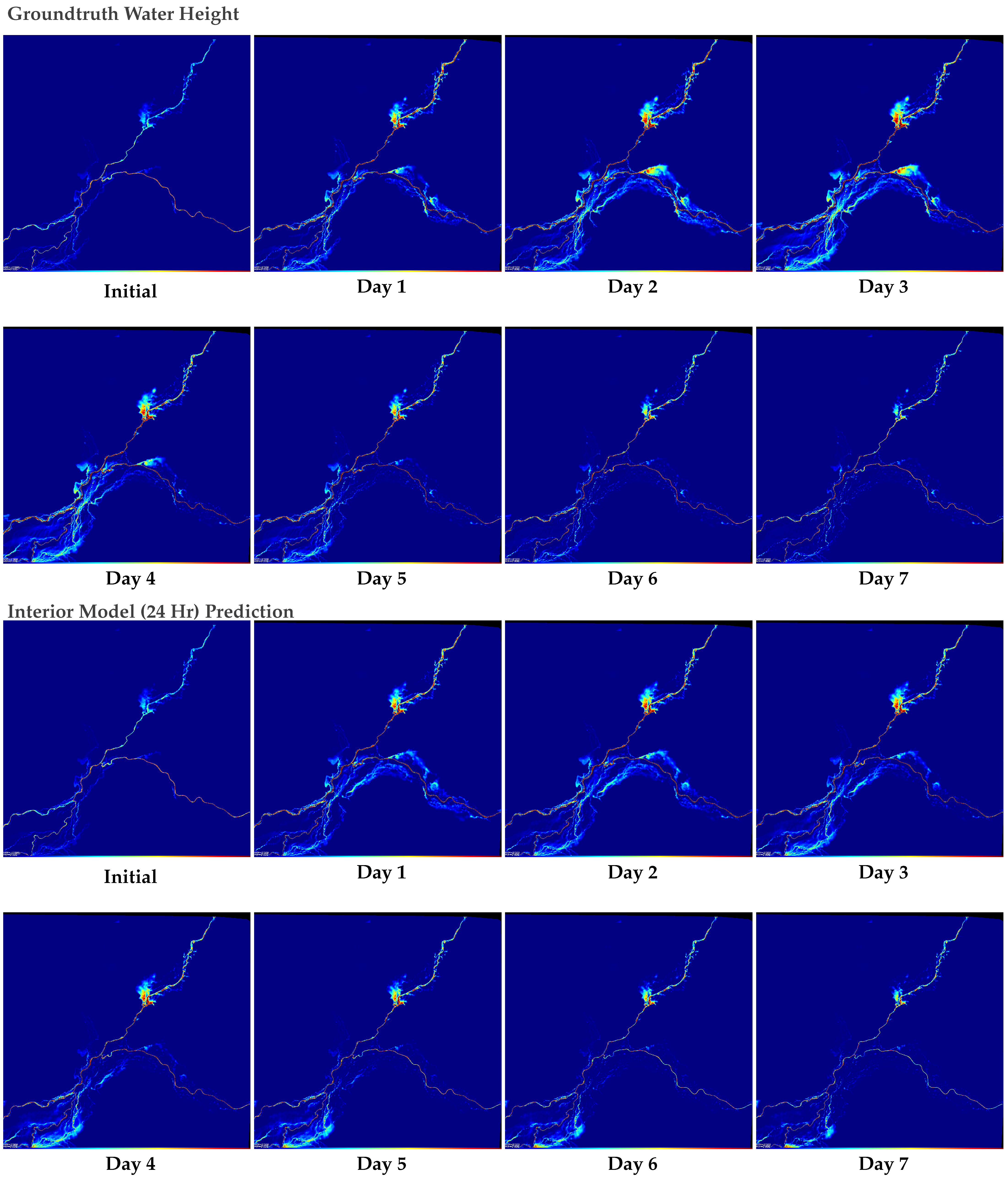
4.2. Interior Model
5. Timing
6. Discussion
Author Contributions
Funding
Data Availability Statement
Conflicts of Interest
References
- Bulti, D.T.; Abebe, B.G. A review of flood modeling methods for urban pluvial flood application. Model. Earth Syst. Environ. 2020, 6, 1293–1302. [Google Scholar] [CrossRef]
- Liu, Q.; Qin, Y.; Zhang, Y.; Li, Z. A coupled 1D–2D hydrodynamic model for flood simulation in flood detention basin. Nat. Hazards 2015, 75, 1303–1325. [Google Scholar] [CrossRef]
- Teng, J.; Jakeman, A.; Vaze, J.; Croke, B.; Dutta, D.; Kim, S. Flood inundation modelling: A review of methods, recent advances and uncertainty analysis. Environ. Model. Softw. 2017, 90, 201–216. [Google Scholar] [CrossRef]
- Kalyanapu, A.J.; Shankar, S.; Pardyjak, E.R.; Judi, D.R.; Burian, S.J. Assessment of GPU computational enhancement to a 2D flood model. Environ. Model. Softw. 2011, 26, 1009–1016. [Google Scholar] [CrossRef]
- Wu, L.; Tong, J.; Wang, Z.; Li, J.; Li, M.; Li, H.; Feng, Y. Post-flood disaster damaged houses classification based on dual-view image fusion and Concentration-Based Attention Module. Sustain. Cities Soc. 2024, 103, 105234. [Google Scholar] [CrossRef]
- Mudashiru, R.B.; Sabtu, N.; Abustan, I.; Waheed, B. Flood Hazard Mapping Methods: A Review. J. Hydrol. 2021, 603, 126846. [Google Scholar] [CrossRef]
- Hosseiny, H. A Deep Learning Model for Predicting River Flood Depth and Extent. Environ. Model. Softw. 2021, 145, 105186. [Google Scholar] [CrossRef]
- Hosseiny, H.; Nazari, F.; Smith, V.; Nataraj, C. A framework for modeling flood depth using a hybrid of hydraulics and machine learning. Sci. Rep. 2020, 10, 8222. [Google Scholar] [CrossRef] [PubMed]
- Rumelhart, D.E.; Hinton, G.E.; Williams, R.J. Learning Representations by Back-propagating Errors. Nature 1986, 323, 533–536. [Google Scholar] [CrossRef]
- Hochreiter, S.; Schmidhuber, J. Long Short-Term Memory. Neural Comput. 1997, 9, 1735–1780. [Google Scholar] [CrossRef] [PubMed]
- Vaswani, A.; Shazeer, N.; Parmar, N.; Uszkoreit, J.; Jones, L.; Gomez, A.N.; Kaiser, L.u.; Polosukhin, I. Attention is All you Need. In Advances in Neural Information Processing Systems; Guyon, I., Luxburg, U.V., Bengio, S., Wallach, H., Fergus, R., Vishwanathan, S., Garnett, R., Eds.; Curran Associates, Inc.: Red Hook, NY, USA, 2017; Volume 30. [Google Scholar]
- Chu, H.; Wu, W.; Wang, Q.; Nathan, R.; Wei, J. An ANN-based emulation modelling framework for flood inundation modelling: Application, challenges and future directions. Environ. Model. Softw. 2020, 124, 104587. [Google Scholar] [CrossRef]
- Zhou, Y.; Wu, W.; Nathan, R.; Wang, Q.J. A rapid flood inundation modelling framework using deep learning with spatial reduction and reconstruction. Environ. Model. Softw. 2021, 143, 105112. [Google Scholar] [CrossRef]
- Nelson. iRIC Software. Available online: https://i-ric.org/en/download/fastmech-examples/ (accessed on 9 November 2021).
- Huxley, C.; Syme, B. TUFLOW GPU-best practice advice for hydrologic and hydraulic model simulations. In Proceedings of the 37th Hydrology &Water Resources Symposium, Queenstown, New Zealand, 28 November–2 December 2016; pp. 195–203. [Google Scholar]
- DHI. MIKE21 Flow Model FM, Hydrodynamic Module, User Guide; DHI Water and Environment Pty Ltd.: Horsholm, Denmark, 2016. [Google Scholar]
- Löwe, R.; Böhm, J.; Jensen, D.G.; Leandro, J.; Rasmussen, S.H. U-FLOOD–Topographic deep learning for predicting urban pluvial flood water depth. J. Hydrol. 2021, 603, 126898. [Google Scholar] [CrossRef]
- Hofmann, J.; Schüttrumpf, H. floodGAN: Using Deep Adversarial Learning to Predict Pluvial Flooding in Real Time. Water 2021, 13, 2255. [Google Scholar] [CrossRef]
- Gallant, J.C.; Dowling, T.I.; Rawntp, C.I. SRTM-Derived 1 s Digital Elevation Models Version 1.0. 2011. Available online: https://data.gov.au/dataset/ds-ga-aac46307-fce8-449d-e044-00144fdd4fa6/details?q= (accessed on 12 August 2021).
- Kumar, S.K. On weight initialization in deep neural networks. arXiv 2017, arXiv:1704.08863. [Google Scholar]
- He, K.; Zhang, X.; Ren, S.; Sun, J. Deep Residual Learning for Image Recognition. In Proceedings of the 2016 IEEE Conference on Computer Vision and Pattern Recognition (CVPR), Las Vegas, NV, USA, 27–30 June 2016; pp. 770–778. [Google Scholar] [CrossRef]
- Ioffe, S.; Szegedy, C. Batch Normalization: Accelerating Deep Network Training by Reducing Internal Covariate Shift. In Proceedings of the 32nd International Conference on Machine Learning, Lille, France, 7–9 July 2015; Bach, F., Blei, D., Eds.; Proceedings of Machine Learning Research. Journal of Machine Learning Research Inc. (JMLR): New York, NY, USA, 2015; Volume 37, pp. 448–456. [Google Scholar]

| Type | Format | Description |
|---|---|---|
| DEM and water height | XYZ text file | Comma separated vertex data storing (x,y) position of triangle mesh point, DEM elevation with respect to Australian Height Datum (AHD, m) and water height above ground (m). Generated by the MIKE 21 model at hourly interval. DEM data is constructed by merging coarse satellite DEM data with fine aerial LIDAR captured directly over the major river [19]. |
| Roughness parameter | GDAL .asc file | Binary data in GDAL format defining surface roughness parameter over a 30 m × 30 m dense grid. Note this grid may not precisely align with the desired input grid. |
| Driving Inflows | CSV text file | Comma separated text data defining the flow-rates at the 3 inflow boundaries sampled daily. Missing data is replaced with an empty string. Data is based on real water gauge observations provided by the Western Australia government. |
| Type | Format | Description |
|---|---|---|
| Water height sequence | vector of float32 matrix | A sequence of water heights for the local region |
| Topological DEM | float32 matrix | The elevation T for the local region |
| Roughness | float32 matrix | The roughness parameter for the local region |
| Mask | boolean matrix | This mask indicates which point in the above matrices contain valid data. This is necessary when near the edge of the dataset where we have missing data. |
| Driving Inflows | float32 vector | Driving inflows at each inflow boundary associated with each water height |
| Metadata | JSON | Additional metadata including timestamps associated with each water height, region bounding box, etc. |
| Block Type | Multi. | Output Dim | Description |
|---|---|---|---|
| Transform | Takes local inputs (flow, topographic DEM data, driving inflows, etc.) and applies the transforms described in Section 3.1. | ||
| Conv-ReLU | Applies a convolution, batch normalization ([22]) and rectified linear (ReLU) activation to the input tensor. | ||
| ResNet | Applies two Conv-ReLU blocks to the input then combines the resulting tensor with the input via an addition operation. The first ResNet block in each sequence downscales the input by [21]. | ||
| ResNet | |||
| ResNet | |||
| ResNet | |||
| ResNet | |||
| Upsample | Applies a upscaling operation to the input, adds the features from the previous defined ResNet block with the same spatial resolution (i.e., skip connection), then applies a basic Conv-ReLU block. | ||
| Upsample | |||
| Upsample | |||
| Upsample | |||
| Upsample | |||
| Regression | Applies a convolution operation with 2 output features to generate the water height change and inundation probability outputs. The water height change is multiplied by scalar constant (in this case 0.001) to improve training dynamics. |
| Model | Day 1 | Day 2 | Day 3 | Day 4 | Day 5 | Day 6 | Day 7 |
|---|---|---|---|---|---|---|---|
| Without driving inflows | 0.378 | 0.527 | 0.295 | 0.348 | 0.562 | 0.683 | 0.750 |
| With driving inflows | 0.109 | 0.208 | 0.120 | 0.148 | 0.188 | 0.195 | 0.200 |
| Method | Hardware | Days | Area | Runtime | Per Day Per 1000 |
|---|---|---|---|---|---|
| MIKE21 | Tesla P100 | 40 | 35,026 | 38 h | 97.6 s |
| ML System | 1080 Ti | 7 | 8242 | 1 min 36 s | 1.7 s |
Disclaimer/Publisher’s Note: The statements, opinions and data contained in all publications are solely those of the individual author(s) and contributor(s) and not of MDPI and/or the editor(s). MDPI and/or the editor(s) disclaim responsibility for any injury to people or property resulting from any ideas, methods, instructions or products referred to in the content. |
© 2024 by the authors. Licensee MDPI, Basel, Switzerland. This article is an open access article distributed under the terms and conditions of the Creative Commons Attribution (CC BY) license (https://creativecommons.org/licenses/by/4.0/).
Share and Cite
Tychsen-Smith, L.; Armin, M.A.; Karim, F. Towards Non-Region Specific Large-Scale Inundation Modelling with Machine Learning Methods. Water 2024, 16, 2263. https://doi.org/10.3390/w16162263
Tychsen-Smith L, Armin MA, Karim F. Towards Non-Region Specific Large-Scale Inundation Modelling with Machine Learning Methods. Water. 2024; 16(16):2263. https://doi.org/10.3390/w16162263
Chicago/Turabian StyleTychsen-Smith, Lachlan, Mohammad Ali Armin, and Fazlul Karim. 2024. "Towards Non-Region Specific Large-Scale Inundation Modelling with Machine Learning Methods" Water 16, no. 16: 2263. https://doi.org/10.3390/w16162263
APA StyleTychsen-Smith, L., Armin, M. A., & Karim, F. (2024). Towards Non-Region Specific Large-Scale Inundation Modelling with Machine Learning Methods. Water, 16(16), 2263. https://doi.org/10.3390/w16162263