Article

Analysis of Surface Water Area Changes and Driving Factors in the Tumen River Basin (China and North Korea) Using Google Earth Engine (2015–2023)

by
Di Wu
1,
Donghe Quan
1 and
Ri Jin
1,2,*
1
College of Geography and Ocean Sciences, Yanbian University, Hunchun 133300, China
2
Northeast Asian Research Center of Transboundary Disaster Risk and Ecological Security, Yanbian University, Hunchun 133300, China
*
Author to whom correspondence should be addressed.
Water 2024, 16(15), 2185; https://doi.org/10.3390/w16152185
Submission received: 27 June 2024 / Revised: 29 July 2024 / Accepted: 31 July 2024 / Published: 1 August 2024

Abstract

:
Understanding the dynamics of water bodies is crucial for managing water resources and protecting ecosystems, especially in regions prone to climatic extremes. The Tumen River Basin, a transboundary area in Northeast Asia, has seen significant water body changes influenced by natural and anthropogenic factors. Using Landsat 8 and Sentinel-1 data on Google Earth Engine, we systematically analyzed the spatiotemporal variations and drivers of water body changes in this basin from 2015 to 2023. The water body extraction process demonstrated high accuracy, with overall precision rates of 95.75% for Landsat 8 and 98.25% for Sentinel-1. Despite observed annual fluctuations, the overall water area exhibited an increasing trend, notably peaking in 2016 due to an extraordinary flood event. Emerging Hot Spot Analysis revealed upstream areas as declining cold spots and downstream regions as increasing hot spots, with artificial water bodies showing a growth trend. Utilizing Random Forest Regression, key factors such as precipitation, potential evaporation, population density, bare land, and wetlands were identified, accounting for approximately 81.9–85.3% of the observed variations in the water body area. During the anomalous flood period from June to September 2016, the Geographically Weighted Regression (GWR) model underscored the predominant influence of precipitation, potential evaporation, and population density at the sub-basin scale. These findings provide critical insights for strategic water resource management and environmental conservation in the Tumen River Basin.

1. Introduction

Surface water is indispensable for human survival, development, and plays a pivotal role in regional economic and social advancement [1,2]. It encompasses natural features such as rivers, lakes, and ponds, as well as constructed reservoirs, channels, and canals. Surface water critically regulates terrestrial hydrological processes, sustains ecological equilibrium, and ensures water availability [3,4,5]. Despite covering a relatively small fraction of Earth’s landmass, it constitutes crucial water resources essential for the majority of urban inhabitants [6]. However, contemporary challenges, including climate change, industrial and agricultural expansion, and population growth, have profoundly impacted water resources, precipitating substantial alterations in hydrological cycles [7,8,9]. Hence, acquiring timely and precise hydrological data and comprehending its spatiotemporal variability are essential for the rational advancement and optimal utilization of water resources, effective terrestrial ecosystem management, and the attainment of sustainable socio-economic development. The rapid advancement of remote sensing technology has provided crucial support for water research [10,11,12], particularly with the emergence of Google Earth Engine (GEE) as a robust cloud computing platform. GEE has significantly simplified the complexity of studying spatiotemporal variations in water within watersheds [13,14]. As a crucial region at the junction of China, North Korea, and Russia, the water resources of the Tumen River Basin are a key component of ecological environmental protection and high-quality development in the area. In-depth research on the spatiotemporal variations of water in the Tumen River Basin is essential for promoting the sustainable utilization of water resources and the protection of the ecological environment in this region.
Water body extraction methods are critical research topics in the field of remote sensing, especially concerning Synthetic Aperture Radar (SAR) satellite imagery. Commonly used water body extraction methods include visual interpretation, threshold segmentation, and object-based classification [15,16,17]. Among these methods, threshold segmentation is widely used due to its simplicity, stability, and efficiency [18,19]. By combining band operations and threshold segmentation methods, along with processing radar imagery using Digital Elevation Model (DEM) data, accurate extraction of water body information can be achieved [20]. Furthermore, the Otsu’s (Otsu) binarization threshold segmentation method can be used to segment the imagery of the monitored area. Combined with DEM data as a slope constraint, this approach enables the preliminary extraction of water bodies [21]. Considering the characteristic that water pixels in SAR imagery exhibit low values while background pixels show high values, the Sentinel-1 Dual-Polarized Water Index (SDWI) was proposed to enhance this feature, making it easier to determine the optimal threshold for segmentation [22,23,24]. To address potential misclassification in areas with significant topographic variation, an improved Otsu threshold segmentation method combining SDWI with terrain factors was proposed. This approach enhances the accuracy and efficiency of water body extraction [25,26]. On the other hand, research on water body extraction based on the GEE has rapidly developed in recent years. GEE, as a cloud computing platform, provides users with extensive Earth observation data and powerful computational capabilities, supporting global-scale Earth science research and environmental monitoring [27,28,29,30,31,32]. Through the GEE, users can efficiently process and analyze remote sensing data, enabling the monitoring and analysis of water bodies over large areas and extended time periods [33,34,35]. Utilizing the GEE in combination with multi-source remote sensing data, such as Sentinel-2 and Landsat imagery, allows for the monitoring and assessment of dynamic water body changes [36]. This includes tracking water dynamics with high temporal resolution, analyzing long-term changes in sedimentation areas [36], and evaluating flood dynamics [37]. These applications demonstrate the significant role of the GEE in water body monitoring. By fully leveraging GEE’s data and computational resources, these studies provide robust support for global water resource management and environmental monitoring.
With the rapid development of cloud computing platforms and the open access to a vast array of data sources, the quantity and variety of water datasets continue to increase globally and regionally. This trend has propelled the direction of water change research. Historically, studies primarily focused on analyzing water changes over several discrete time slices. However, with technological advancements, researchers now prefer using long-term continuous time series data to achieve more scientific and comprehensive results [38]. For example, Belward et al. utilized the GEE in conjunction with 30 years of Landsat satellite imagery and expert system water body extraction methods, discovering that the area of permanent water bodies has increased in most regions [32]. Ji et al. used MODIS data to create a global daily water cover dataset, which is employed for detecting phenomena such as sea level rise [39]. In studying the driving mechanisms of water area changes, researchers have often relied on traditional methods such as multiple linear regression and Pearson correlation analysis to assess the impacts of climatic factors and human activities [40]. However, emerging methods like Random Forest Regression and GWR are gaining attention. Random Forest Regression can handle nonlinear relationships, automatically manage interactions between features, and exhibit robustness against outliers and missing values, making it advantageous for studying water area changes [41]. GWR takes into account spatial dependencies among data, providing a more accurate reflection of spatial relationships and offering a more reliable spatial interpretation of the analysis results [42]. The application of these methods opens up new avenues and possibilities for researching the driving mechanisms behind water area changes, enhancing the depth and reliability of such studies.
This study aims to utilize the GEE, combined with remote sensing data from the Sentinel-1 and Landsat satellite series, to extract and analyze water in the Tumen River Basin from June to September during the period 2015–2023. By examining the distribution and area changes of water, the study employs Emerging Hot Spot Analysis methods to reveal the spatiotemporal evolution trends and characteristics of water area changes at both the grid and sub-basin scales. Random Forest Regression is used to explore the impacts of various variables on water area changes in the Tumen River Basin, including precipitation, potential evaporation, elevation, slope, aspect, land use type, population density, and river density. By comparing the results obtained at different scales, a deeper understanding of the impacts of these factors on driving water area changes is achieved. To further account for spatial heterogeneity, the GWR model is applied, particularly focusing on the year 2016, which saw the most significant changes in water area. The GWR model is used to study the relationships between water area changes and various influencing factors at both the grid and sub-basin scales. This research provides practical experience and methodological references for the application of remote sensing technology in water resource studies, offering important theoretical and practical significance.

2. Materials and Methods

2.1. Study Area

The Tumen River Basin, located in Northeast Asia, is an important transboundary watershed. The basin is primarily drained by the Tumen River, a significant river in Northeast Asia that serves as the boundary between China and North Korea. The study area selected for this research is approximately bounded by 128°00′00″ to 131°19′56″ E and 41°11′20″ to 44°02′32″ N, covering a total area of about 33,300 km2. The Chinese side accounts for approximately 22,700 km2, making up 68.17% of the study area, while the North Korean side covers about 10,600 km2, constituting 31.83% of the study area. The region features diverse topography, including hills, mountains, and river valleys. It is densely populated and serves as a major agricultural production base, primarily cultivating rice, corn, soybeans, and other crops. The basin has abundant water and forest resources, which are of significant importance to the local economy and ecological environment. The climate is characterized as temperate monsoon, with warm, rainy summers and cold, dry winters. Precipitation from June to September accounts for approximately 70% of the annual total, indicating that summer is the season with the most abundant rainfall in the area. The location of the Tumen River Basin is illustrated in Figure 1.

2.2. Datasets and Preprocessing

2.2.1. Remote Sensing Data

(1)
Sentinel-1 SAR
The Sentinel-1 satellite, operated by the European Space Agency as part of the Copernicus program, is equipped with a C-band radar imaging system. It provides four imaging modes: Interferometric Wide Swath (IW), StripMap (SM), Extra Wide Swath (EW), and Wave (WV). The dual-satellite configuration of Sentinel-1 enables a revisit period of 6 days, allowing frequent updates to Earth surface observations. Renowned for its high spatial resolution of up to 5 m, Sentinel-1 can capture fine-scale changes on the ground reliably under various cloud cover and weather conditions, making it an ideal choice for monitoring geological hazards and environmental changes, such as water body extraction, flood monitoring, and landslide detection.
This study utilized data from the GEE covering the period from 2015 to 2023, primarily focusing on the months of June to September each year. Ground Range Detected (GRD) products were selected that underwent preprocessing, including atmospheric and geometric corrections, making them more suitable for water body extraction applications. GRD products have high spatial resolution and two polarization modes: Vertical Horizontal (VH) and Vertical Vertical (VV). The VV polarization mode was mainly used for water body extraction, as it is typically more effective than the VH polarization mode, with higher reflectance and clearer contrast for water bodies under VV polarization. Using the code segment ee.ImageCollection(“COPERNICUS/S1_GRD”), Sentinel-1 SAR data were retrieved from the GEE, clipped, and subjected to terrain correction and filtering. A custom terrain correction function was applied to perform terrain correction on the input SAR image collection, generating two differently corrected images. Subsequently, the average values of the original SAR image collection and the two corrected images were printed. A filtering function was then defined to process the images, and the filtered image bands were added to the original image collection. The average values of the VV and VH bands in the filtered image collection were computed and merged into one image. Finally, the merged image was printed to enhance the quality of the SAR image.
(2)
Landsat data
However, it was observed that the data for the year 2016 was missing when using Sentinel-1 data. Therefore, Landsat 8 data for the year 2016 was selected to fill this gap. The code segment ee.ImageCollection(“LANDSAT/LC08/C02/T1_L2”) was used to retrieve Landsat 8 data from the GEE, which were then clipped and subjected to cloud removal processing. First, masks representing clouds and shadows were defined. Then, QA pixels were extracted from the images, and bitwise and logical operations were performed to determine which pixels belonged to clouds and shadows. Finally, the generated masks were used to update the images, setting the cloud and shadow portions to invalid values or removing them from the images, thus producing clear images unaffected by clouds and shadows.

2.2.2. Factors Influencing the Spatial and Temporal Variability of Surface Water

(1)
Meteorological Data
Meteorological data were stored in NetCDF format, and the Climate Data Operators (CDO) tool was utilized for its rich set of commands and functions that efficiently process large-scale meteorological datasets. This study employed CDO tools, along with Python, to perform batch clipping (sellonlatbox), temporal merging (mergetime), and summation (monsum) operations on the meteorological data to obtain the cumulative precipitation data and cumulative potential evaporation data for June to September from 2015 to 2023.
(2)
Digital Elevation Model (DEM)
The DEM data for the study area were processed using the “Mosaic To New Raster” and “Clip Raster” tools in ArcGIS Pro, a geographic information system software. For more information, see https://www.esri.com/en-us/arcgis/products/arcgis-pro/overview (accessed on 10 June 2024). Subsequently, the Surface Analysis tools in ArcToolbox were used to derive the slope and aspect of the study area. After performing Surface Analysis in ArcGIS, the original aspect map was obtained. The aspect was then converted into a continuous variable using the following formula:
ORI_aspect = 1 2 ( aspect π π ) 2
In this formula, “ORI_aspect” represents the transformed aspect data, with values ranging between –1 and 1. A value closer to –1 indicates a north-facing slope, while a value closer to 1 indicates a south-facing slope. The aspect is the original aspect value derived from the DEM.
(3)
Other Data Sources
Other data sources include global hydrological data, land use type data, and population density data, as detailed in Table 1. For land use and population density data, which exhibit minimal interannual variation compared to meteorological data, the latest available year was used to fill in any missing years. This approach ensures consistency in the analysis across the entire time frame.

2.3. Methodology

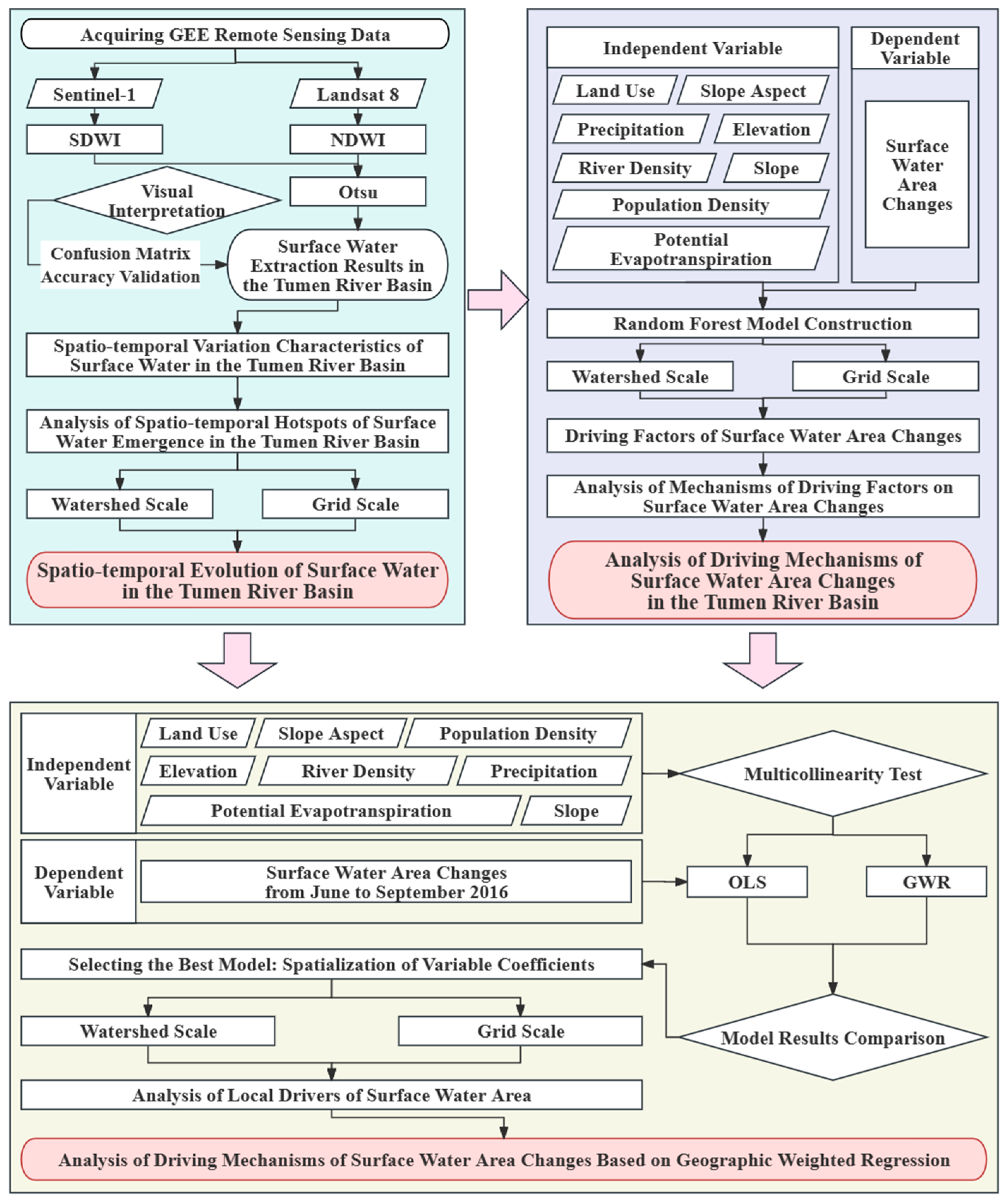
First, Sentinel-1 and Landsat 8 data were processed using the SDWI and the NDWI algorithms, respectively, to distinguish between water and non-water bodies based on the reflectance of different bands in the remote sensing data. Next, Otsu was applied for automatic threshold selection, achieving adaptive binarization of the images to generate binary water body maps. The accuracy of the classification models was then evaluated using a confusion matrix and Kappa coefficient to ensure the reliability of the extraction results, as detailed in Section 2.3.1. The study area was divided into sub-watershed and grid scales, as described in Section 2.3.2. A novel spatiotemporal hot spot analysis was conducted at different scales, as outlined in Section 2.3.3. Based on the changes in the water area from June to September during 2015–2023, Random Forest Regression was employed to investigate the impacts of variables such as precipitation, potential evaporation, elevation, slope, aspect, land use type, population density, and river density on the water area changes in the Tumen River Basin at both the grid and sub-watershed scales. To further consider the spatial heterogeneity, the Geographically Weighted Regression model was applied. For the year 2016, identified as a year with significant changes in the water area, the relationships between water area changes and various variables were studied at the grid and sub-watershed scales. These analyses are detailed in Section 2.3.4. The technical roadmap is illustrated in Figure 2.

2.3.1. Methods for Water Extraction and Accuracy Verification

(1)
Sentinel-1 Dual-Polarized Water Index (SDWI)
For Sentinel-1 SAR data, the SDWI is used to extract water bodies. The formula is as follows [43]:
SDWI = ln 10 × VV × VH 8
The SDWI aims to enhance the features of water bodies, making them more distinguishable from other surface objects. By multiplying the VV and VH polarized images and then scaling by a factor of 10, the reflectance difference between water and non-water areas is amplified. Taking the natural logarithm of the result further emphasizes water characteristics, reduces interference from soil and vegetation, and improves the accuracy and reliability of water information extraction.
(2)
Normalized Difference Water Index (NDWI)
For Landsat 8 data, the NDWI is chosen for water extraction. The formula is [44]
NDWI = Green NIR Green + NIR
The principle of NDWI is that water bodies usually have higher reflectance in the near-infrared (NIR) band than in the visible green band, whereas land surfaces exhibit the opposite behavior. Therefore, the NDWI values for water bodies are typically higher, while those for land areas are lower. By calculating the NDWI, water bodies can be effectively distinguished from land, providing spatial distribution information of water bodies.
(3)
Otsu’s Method (Otsu)
Otsu’s method is used for both Sentinel-1 SAR and Landsat 8 data during the water extraction process [45]. This method, proposed by the Japanese scholar Nobuyuki Otsu in 1979, is an algorithm for determining the binary segmentation threshold of an image, particularly suited for images with bimodal histograms. Known as the maximum between-class variance method, Otsu’s method works by maximizing the variance between the background and the target (foreground) in an image. By doing so, it effectively distinguishes the two parts, ensuring minimal misclassification. The greater the variance between the background and the target, the more distinct the two parts. If parts of the target are misclassified as background or vice versa, this variance decreases. Therefore, selecting the threshold that maximizes the between-class variance minimizes the probability of misclassification. Due to its simplicity and effectiveness, Otsu’s method is widely used in digital image processing.
(4)
Confusion Matrix and Kappa Coefficient
The confusion matrix and Kappa coefficient are used to evaluate the accuracy of water extraction results [46,47]. The confusion matrix is a two-dimensional table that compares the predictions of the classification model with the actual observations, including true positives (TP), true negatives (TN), false positives (FP), and false negatives (FN). The Kappa coefficient is a metric that measures the performance of a classification model, typically ranging from –1 to 1, indicating the degree of agreement of the classification results. The closer the value is to 1, the better the model’s performance.

2.3.2. Scale Division

When analyzing changes in water bodies, it is essential to consider spatiotemporal hot spots at different scales to reveal the spatial and temporal characteristics of water body changes. Water body changes are influenced by various factors, and different patterns may emerge at different scales, necessitating a comprehensive analysis of the changing characteristics across different scales. The driving factors of water body changes involve multiple aspects, and the degree of influence varies at different scales. Therefore, when analyzing these driving factors, it is crucial to consider their impacts at different scales and select appropriate modeling methods accordingly. In summary, analyzing water body changes at different scales contributes to a comprehensive understanding of their patterns, providing essential insights for effective water resource management and environmental protection.
(1)
Sub-basin Scale
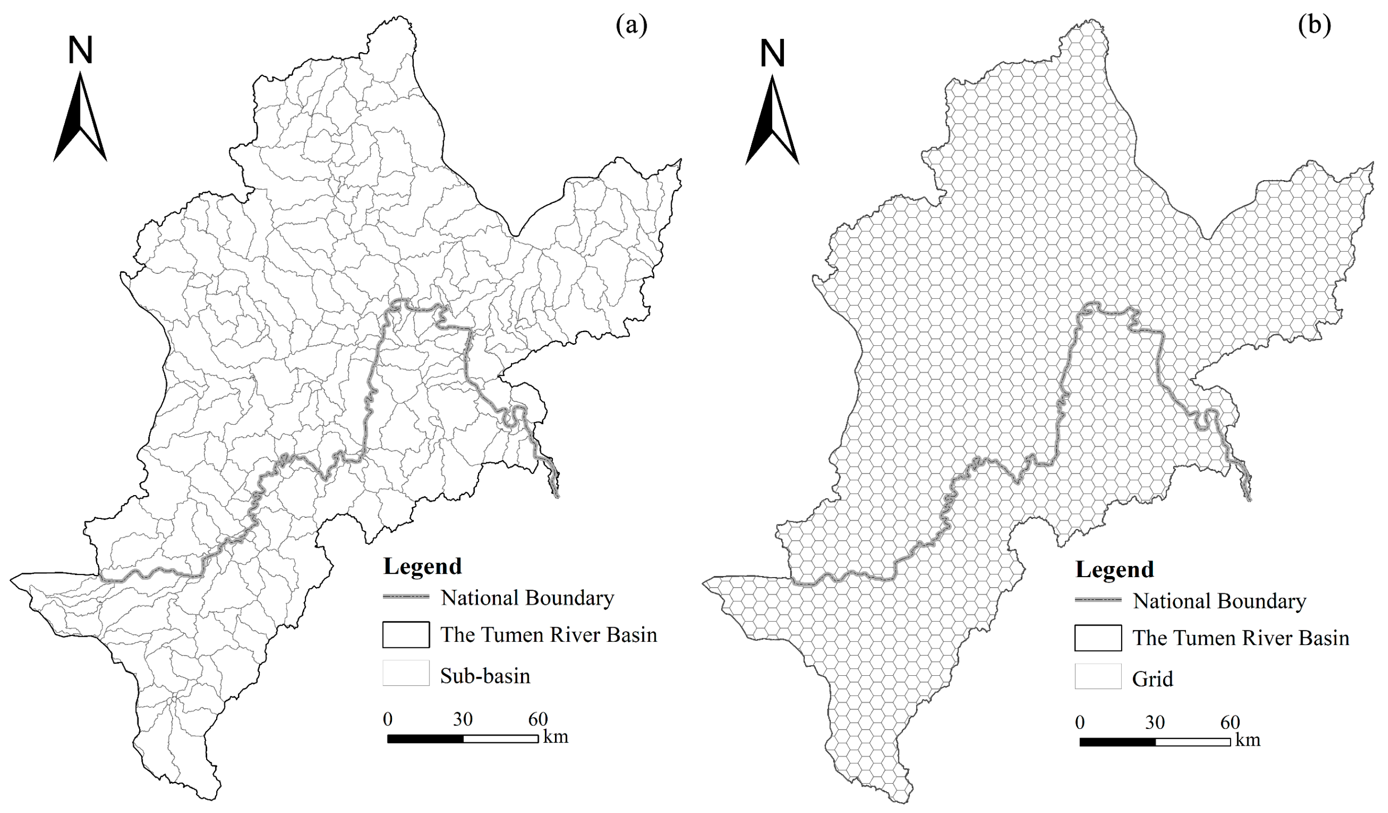
Using the hydrological analysis tools in ArcGIS 10.8, the river network and catchment areas of the Tumen River Basin were extracted based on Digital Elevation Model (DEM) data. The river network extraction involves identifying and delineating the river distribution within the Tumen River Basin using DEM data, facilitating the subsequent analysis of water body distribution and changes. Catchment extraction delineates the watershed boundaries based on topographic features, aiding in the management and study of water resources within the basin [48]. This process is illustrated in Figure 3a.
(2)
Grid Scale
In this study, a hexagonal grid was used for data analysis. Compared to traditional square grids, hexagonal grids are closer in shape to circles, effectively reducing edge effects and deformation caused by the Earth’s curvature, thereby improving spatial analysis accuracy. After continuous adjustments, the grid area was finalized at 25 km2. The grid was created using the Generate Tessellation tool in ArcGIS Pro, as shown in Figure 3b.

2.3.3. Emerging Hot Spot Analysis

First, the water area samples over time for different spatial locations are structured into a three-dimensional spatiotemporal cube dataset, where the x and y dimensions represent space and the t dimension represents time. Each cube cell represents the water area sample value at a single time step for a specific spatial location. Next, the Getis–Ord Gi* statistic is calculated for each cube cell within the spatiotemporal cube to identify statistically significant spatiotemporal hot spots or cold spots. A cube cell’s Getis–Ord Gi* statistic is considered statistically significant if the False Discovery Rate (FDR) corrected p-value is less than or equal to 0.1. Subsequently, the Mann–Kendall statistic is applied to the time series of Gi* values at each spatial location to perform a trend test. Based on the hot spot or cold spot results for each cube cell, and the trend results from the Mann–Kendall test, the spatiotemporal hot spots or cold spots are classified into eight types: new (first-time significant), consecutive (continuous significance), intensifying (increasing significance), persistent (consistent significance), diminishing (decreasing significance), sporadic (intermittent significance), oscillating (alternating between hot and cold spots), and historical (no longer significant but was significant in the past).
Finally, ArcGIS Pro is used to conduct the emerging spatiotemporal hot spot analysis, with a temporal resolution set to one year and a neighborhood time step set to two years [49]. The Getis–Ord Gi* statistic is computed to assess spatiotemporal clustering. After FDR correction, spatiotemporal hot spots or cold spots with p-values less than or equal to 0.1 are identified as statistically significant. The Mann–Kendall trend test is conducted at a significance level of α = 0.05.

2.3.4. Methodologies for Analyzing Driving Factors

(1)
Random Forest Regression
Random Forest Regression is an ensemble learning method consisting of multiple decision trees. Each decision tree is trained using randomly sampled data and features [50]. In classification problems, Random Forest determines the final classification result through a voting mechanism, while, in regression problems, it averages the predictions of each tree to obtain the final result.
Random Forest is a powerful ensemble learning method that constructs a large number of decision trees to perform classification or regression tasks. During training, N samples are randomly drawn with replacements from the training dataset to form multiple bootstrap samples. For each bootstrap sample, a decision tree is generated. During the construction of each decision tree, m features are randomly selected as candidate variables for node splitting. Typically, m is the square root of the total number of features, M. All decision trees are fully grown without pruning. For prediction, each decision tree classifies the sample, and the final prediction is determined by the majority vote in classification tasks or the average prediction in regression tasks.
When validation samples are unavailable, Random Forest Regression proves to be an effective and feasible method. Additionally, Random Forest Regression can provide information on the relative importance of variables and their partial dependencies, making it a powerful machine learning tool. In this study, Random Forest models are constructed using the randomForest package in R version 4.1.3 to evaluate the importance and partial dependence of different variables at various scales.
(2)
Geographically Weighted Regression (GWR)
Geographically Weighted Regression (GWR) is a spatial regression method designed to explore the spatial relationships between dependent and independent variables [51]. Unlike global regression models, GWR accounts for spatial heterogeneity and spatial dependence by fitting a local regression model at each spatial point. It utilizes a spatial weight matrix to adjust the weights of sample data to reflect spatial correlations.
The GWR model for a specific spatial point i can be represented as
Y i = β 0 i + j = 1 p β j i X j i + ε i
where Y i is the observed value of the dependent variable at spatial point i, X j i is the observed value of the j-th independent variable at spatial point i, β 0 i and β j i are the intercept and regression coefficients at spatial point i, and ε i is the error term.
Compared to the OLS model, the GWR model accounts for the local effects of spatial objects, thus providing higher accuracy. In this study, we utilize the GWR model in ArcGIS Pro to analyze the spatial distribution of the relationships between various factors and changes in the water area. This approach allows for a detailed understanding of how different variables interact with water area changes across space, yielding clearer regression results and more pronounced internal regression differences.

3. Results

3.1. Spatiotemporal Evolution of Water in the Tumen River Basin

3.1.1. Accuracy Assessment of Water Extraction

For the accuracy assessment of water extraction, data from August 2016 and September 2021 were selected as examples for Landsat 8 and Sentinel-1, respectively. A total of 200 water sample points and 200 non-water sample points were randomly generated. These sample points were visually interpreted to validate the accuracy of the water extraction results.
As shown in Table 2 and Table 3, the results indicate that the accuracy of water extraction using Landsat 8 and Sentinel-1 data is 95.75% and 98.25%, respectively, with Kappa coefficients of 0.92 and 0.97. This demonstrates that both datasets perform well in water body extraction, yielding relatively reliable results.

3.1.2. Spatiotemporal Characteristics of Water Changes

As shown in Figure 4, the changes in the water area in the Tumen River Basin from 2015 to 2023 do not exhibit a clear monotonic increasing or decreasing trend. The water area reached its maximum value in 2016. Further analysis can be conducted using the fitted trendline equation. The average annual growth rate of the water area is approximately 0.76 km2 per year, with an initial value of 190.11 km2.

3.1.3. Emerging Hot Spot Analysis in Surface Water

(1)
Sub-watershed Scale
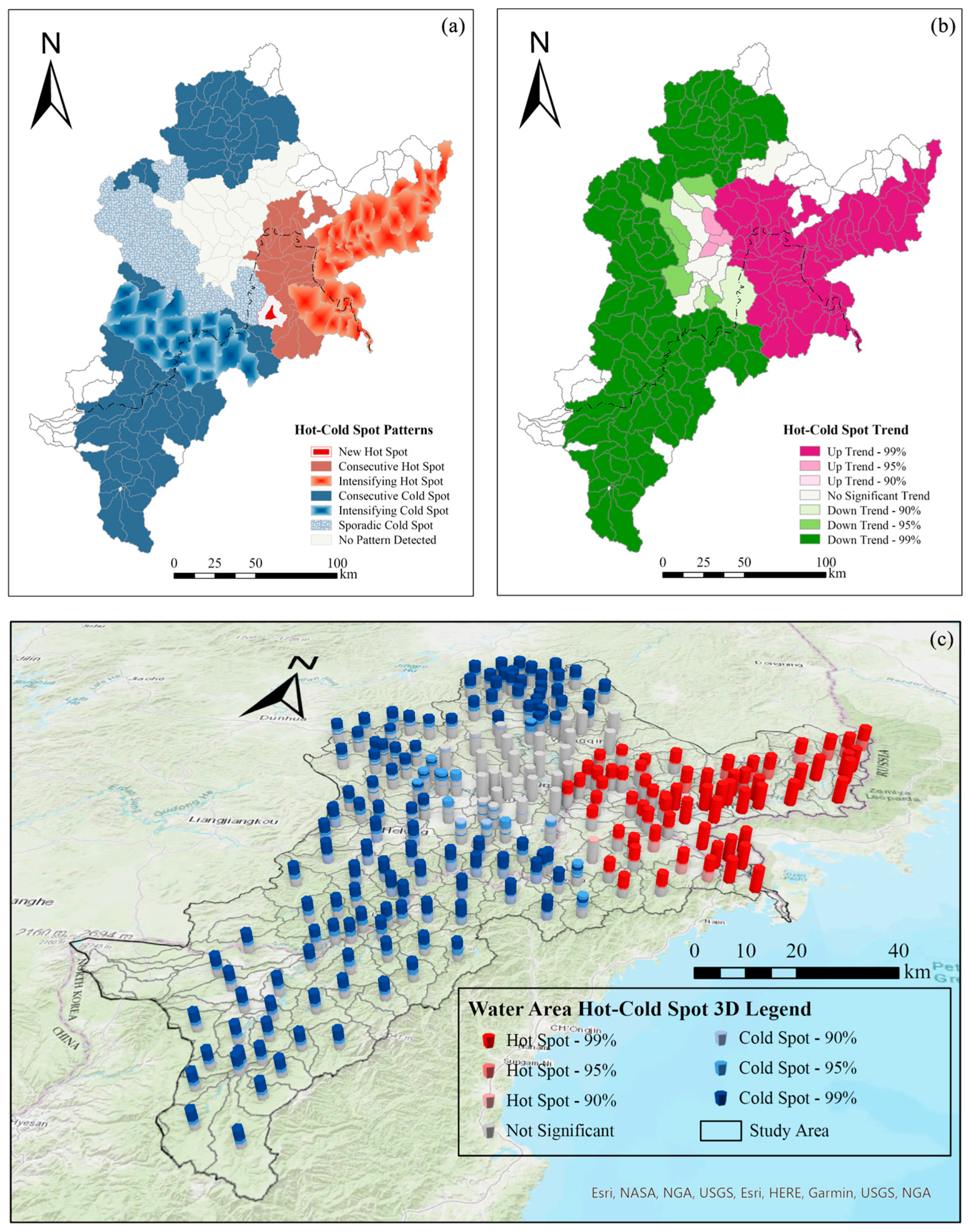
As illustrated in Figure 5, six distinct hot–cold spot patterns of the water area were observed at the sub-watershed scale within the Tumen River Basin. The upper and middle reaches predominantly exhibited cold spots, including continuous, intensifying, and sporadic cold spots. In contrast, the lower reaches showed hot spot patterns, comprising new, continuous, and intensifying hot spots.
Further analysis of the trends in the water area hot–cold spots revealed that the upper and middle reaches primarily experienced a significant decreasing trend, with a confidence level of 99%. This indicates a substantial reduction in water area in these regions. Conversely, the lower reaches demonstrated a significant increasing trend in water area, also at a 99% confidence level, indicating a notable expansion of water in these areas during the study period. The 3D spatial distribution of the hot–cold spots for the water area in the Tumen River Basin provides a more intuitive understanding of the annual variation trends. Each column in the 3D spatial distribution map represents the changes in the hot–cold spots for the water area in different years. By observing the distribution and variation of these columns, the spatial distribution patterns of the hot–cold spots across different years and their temporal evolution can be clearly seen. The upper reaches predominantly featured concentrated cold spots, while the lower reaches exhibited concentrated hot spots, a trend significant at the 99% confidence level. Additionally, the annual fluctuations in the upper, middle, and lower reaches displayed a high degree of consistency.
(2)
Grid Scale
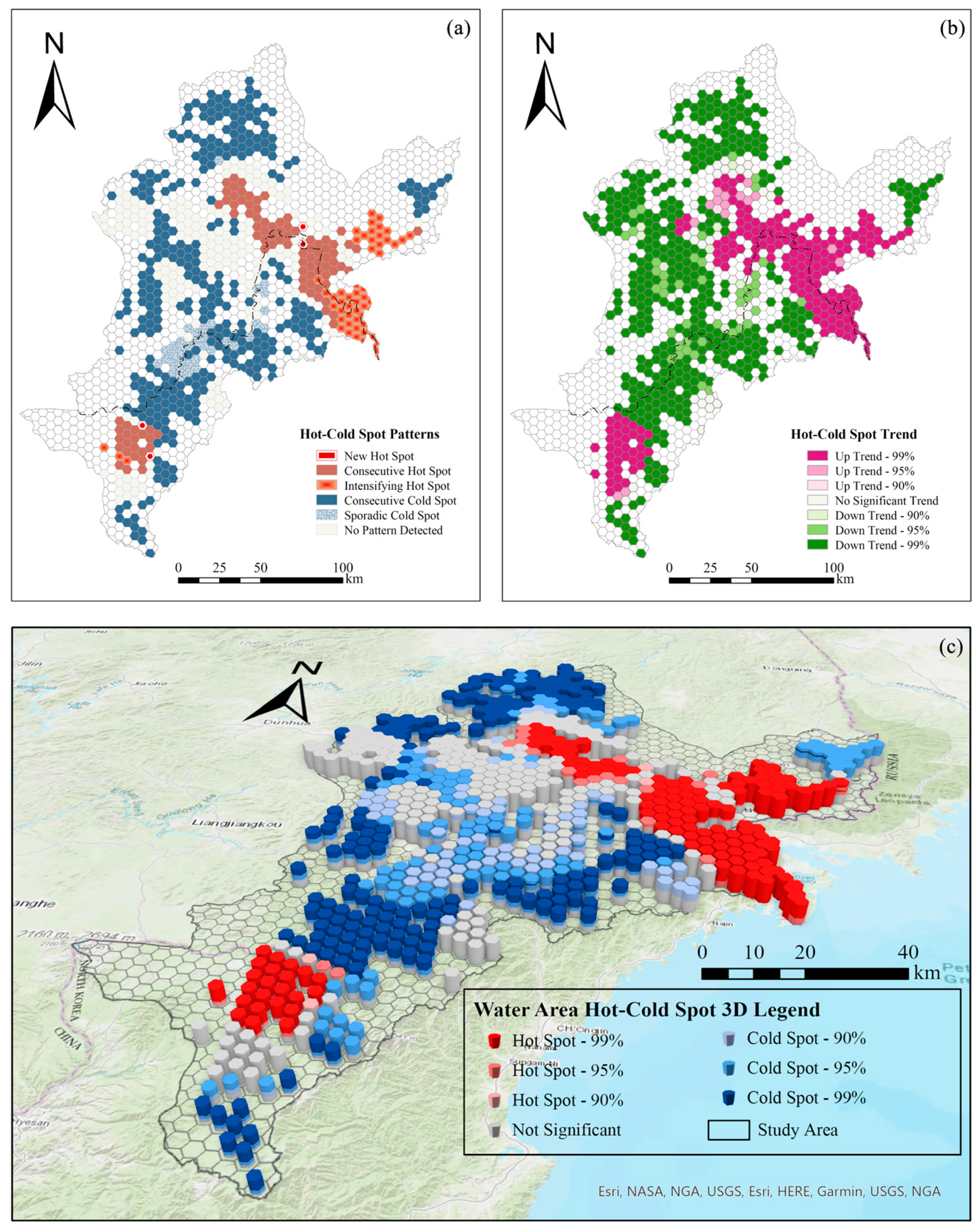
As shown in Figure 6, at the grid scale, the water area in the Tumen River Basin exhibits five types of hot–cold spot patterns. Most of the upper and middle regions are classified as cold spots, including continuous and sporadic cold spots. However, a small portion of the upper reaches displays emerging and continuous hot spots. In contrast, the lower reaches exhibit hot spot patterns, including emerging, continuous, and intensifying hot spots. A further trend analysis of the hot–cold spots reveals that the water area in the upper and middle regions primarily shows a decreasing trend, significant at the 99% confidence level. Conversely, a small part of the upper region exhibits an increasing trend, also significant at the 99% confidence level. The lower region predominantly shows an increasing trend in the water area, which is likewise significant at the 99% confidence level. The spatial distribution indicates a concentration of hot spots in a small portion of the upper reaches and the lower region, while most of the upper and middle regions display a concentration of cold spots. Overall, the annual variation trends in cold and hot spots remain consistent, reflecting the spatiotemporal dynamics of the water area changes in the Tumen River Basin.

3.2. Fitting Results of the Random Forest Regression Model

3.2.1. Model Construction

(1)
Selection of Model Variables and Parameter Settings
In constructing the model for analyzing water area changes at different scales, the dependent variable selected is the change in water area from June to September during the period 2015–2023. The independent variables include precipitation (Pre); potential evapotranspiration (PET); proportions of land use types comprising forests (Trees), wetlands (Paddy), bare land (Bare), croplands (Crops), built-up areas (Built), and rangelands (Rangeland); population density (POP); elevation (DEM); slope (Slope); aspect (Aspect); and river density (River_dens), totaling 13 independent variables. These variables encompass various aspects of the geographical environment, population distribution, and meteorological conditions, thereby providing a comprehensive reflection of the factors driving changes in the water area.
(2)
Model Fit
As shown in Table 4, at the sub-basin scale, the model’s mean squared error (MSE) is 0.131, and the R2 is 0.819. This indicates that, while there is some discrepancy between the model predictions and the actual observed data, the model can explain approximately 81.9% of the variance in the observed data. At the grid scale, the model’s mean squared error is 0.027, and the R2 is 0.853. This demonstrates that, at a more detailed spatial scale, this model’s fit is better, with a higher degree of alignment with the actual observed data, explaining about 85.3% of the variance. Overall, the Random Forest model performs better at the grid scale, showing superior fit, but the models at both scales are capable of accurately predicting changes in water areas.

3.2.2. Relative Importance of Drivers of Water Area Change

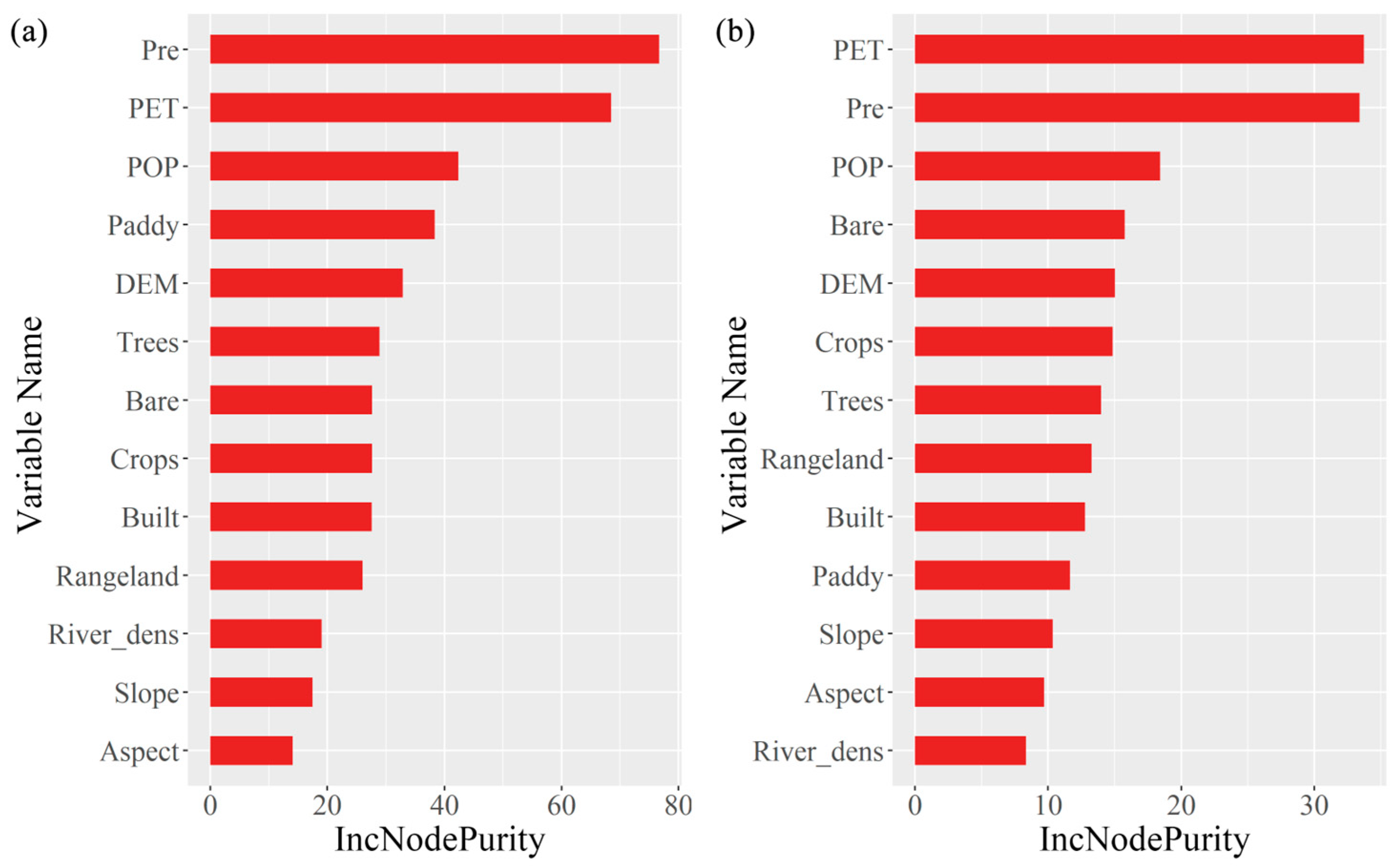
At the sub-basin scale, as illustrated in Figure 7, the relative importance of the variables influencing water area changes from June to September 2015–2023, in descending order, is Pre > PET > POP > Paddy > DEM > Trees > Bare > Crops > Built > Rangeland > River_dens > Slope > Aspect.
At the grid scale, as illustrated in Figure 7, the relative importance of the variables influencing water area changes from June to September 2015–2023, in descending order, is PET > Pre > POP > Bare > DEM > Crops > Trees > Rangeland > Built > Paddy > Slope > Aspect > River_dens.

3.2.3. Partial Dependence Plots for the Driving Factors of Water Area Changes

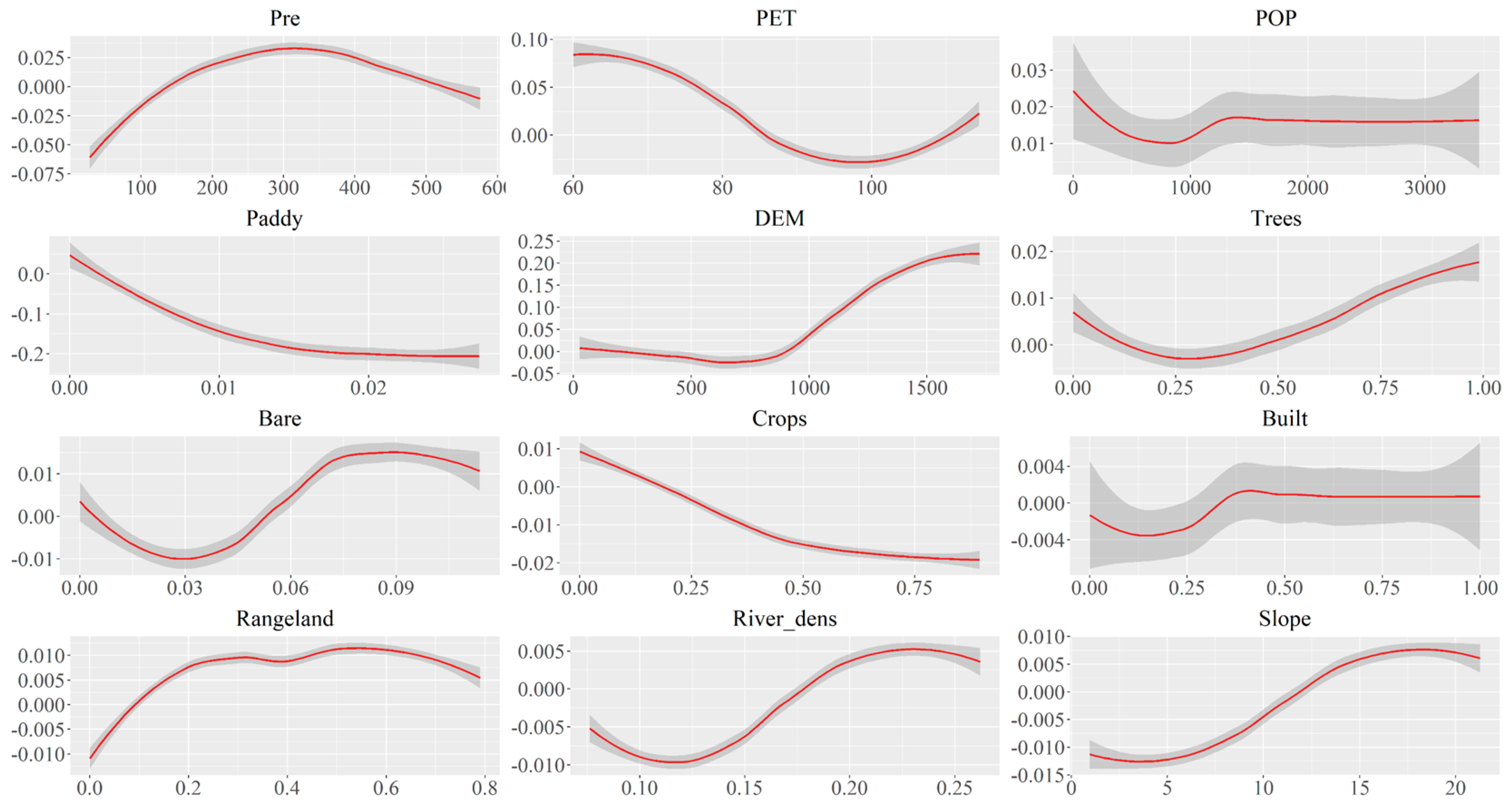
At the sub-basin scale, the influence of various factors on water area changes demonstrates distinct patterns, as shown in Figure 8. Precipitation affects water area expansion significantly up to 300 mm; beyond which, further increases paradoxically slow the rate of change. Potential evapotranspiration (PET) reduces water area changes as it approaches 100 mm; however, beyond this point, the trend reverses, and water area changes begin to increase. Population density impacts are more nuanced: initial increases up to approximately 900 people/km2 correlate with a decrease in water area changes. Between 900 and 1300 people/km2, water area changes escalate, eventually stabilizing beyond 1300 people/km2. The presence of paddy fields shows a consistent negative correlation with water area changes as their proportion rises. Other variables exhibit complex, nonlinear effects. For instance, Digital Elevation Model (DEM), forests (trees), bare land, built-up areas, rangeland, river density, and slope each interact with water area changes in unique, nonlinear ways. In contrast, agricultural land (crops) maintains a linear relationship with water area changes, underscoring its more predictable impact.
At the grid scale, the influences on water area changes share certain similarities with those observed at the sub-basin scale, as depicted in Figure 9. The effects of precipitation and potential evapotranspiration (PET) on water area changes are highly consistent with the patterns observed at the sub-basin scale. Population density also follows a comparable pattern: water area changes decrease as the density increases from low values up to approximately 5000 people/km2, then rise between 5000 and 10,000 people/km2, and eventually stabilize when the density exceeds 10,000 people/km2. An increase in the proportion of bare land consistently results in a gradual decrease in water area changes. Other factors, including the Digital Elevation Model (DEM), forests, built-up areas, river density, and slope, exhibit nonlinear relationships with water area changes, each influencing the hydrological dynamics in distinct, complex ways. In contrast, rangeland and agricultural land (crops) maintain a linear relationship with changes in the water area, suggesting more straightforward interactions.

3.3. Fitting Results of the Geographically Weighted Regression Model

While Random Forests are proficient at capturing complex relationships within spatial data, their interpretability is limited. In contrast, GWR provides interpretable results, making it particularly suitable for exploring local spatial variation patterns. By leveraging the strengths of both methods, this study employs the GWR model to analyze the changes in the water area for the year 2016. This year is considered anomalous due to the maximum water area recorded between June and September during the period of 2015–2023. By accounting for spatial correlation, the analysis aims to investigate key factors and their spatial relationships.

3.3.1. Model Construction

(1)
Multicollinearity Test Results
In this study, the variance inflation factor (VIF) was employed to test for multicollinearity among the independent variables, aiming to exclude those with significant multicollinearity. Typically, VIF values are greater than 1, and values exceeding 10 may indicate severe multicollinearity. By removing variables with high VIF values, the model’s robustness and interpretability are improved. After conducting the multicollinearity test, variables such as wetlands, croplands, and grasslands were excluded due to their high correlation with other variables, which could potentially affect the model’s accuracy (Table 5).
(2)
Comparison of Model Goodness of Fit
This study uses R2, adjusted R2, and corrected Akaike Information Criterion (AICc) to evaluate the goodness of fit of the models (Table 6). The results indicate that the GWR model performs slightly better than the OLS model. Therefore, the GWR model was selected to analyze the changes in the water area in the Tumen River Basin in 2016, incorporating 10 independent variables: Pre; PET; land use types; POP; and topographic factors (DEM, slope, aspect, and river density). The GWR analysis allows for the examination of the spatial influence of these factors.

3.3.2. Spatial Distribution of Regression Coefficients for the Driving Factors of Water Area Changes

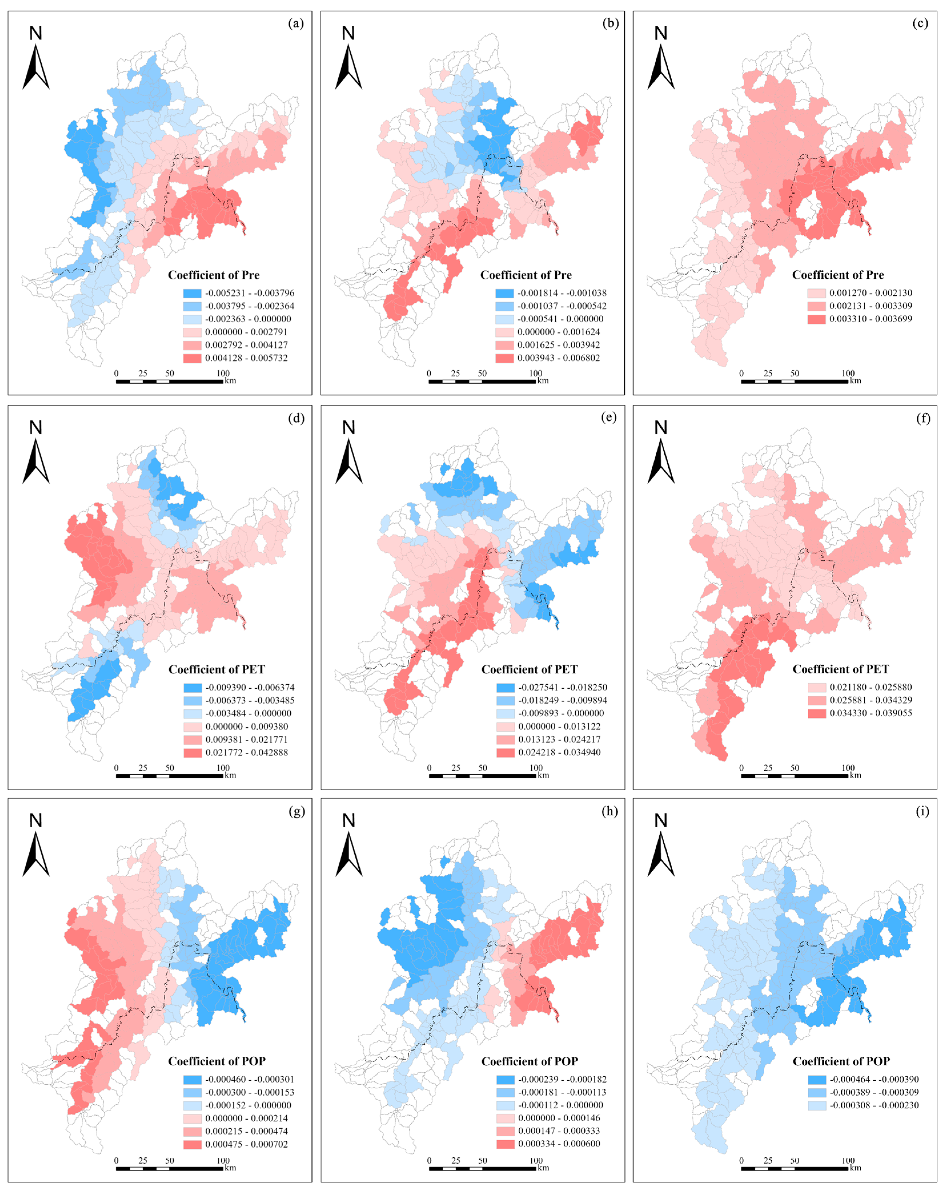
At the sub-basin scale, as detailed in Section 3.2, precipitation (Pre), potential evapotranspiration (PET), and population density (POP) emerge as significant drivers of water area changes within the Random Forest Regression model.
Precipitation influences water areas differently across regions and time periods (Figure 10a–c). From June to July, water area changes in China and North Korea shift from a negative to a positive correlation. By July to August, China’s upper reaches show a positive correlation, the middle reaches a negative correlation, and the lower reaches return to a positive correlation. North Korea follows a similar pattern: strong positive correlations in the upper reaches, negative in the middle reaches, and positive again downstream. Moving into August to September, both countries consistently exhibit positive correlations, with the relationship intensifying from upstream to downstream.
Potential evapotranspiration (PET) also displays varying impacts (Figure 10d–f). In June to July, China’s upper reaches show a positive correlation, the middle reaches a negative correlation, and the lower reaches again a positive but weaker correlation. In North Korea, the upper reaches exhibit a negative correlation, whereas the middle and lower reaches are positively correlated. From July to August, positive correlations dominate China’s upper reaches, while negative correlations appear downstream. In North Korea, strong positive correlations are observed in the upper reaches, contrasting with negative correlations downstream. By August to September, both nations show positive correlations throughout, with North Korea’s upper reaches displaying the most pronounced positive correlation.
Population density (POP) impacts water area changes with distinct temporal and spatial patterns (Figure 10g–i). Between June and July, the regions in both China and North Korea transition from a negative to a positive correlation. During July to August, China’s middle reaches exhibit a negative correlation, while the lower reaches are positively correlated. North Korea exhibits a more pronounced negative correlation compared to China during this period. From August to September, both nations show negative correlations across all regions, with the strength of this correlation increasing from upstream to downstream.
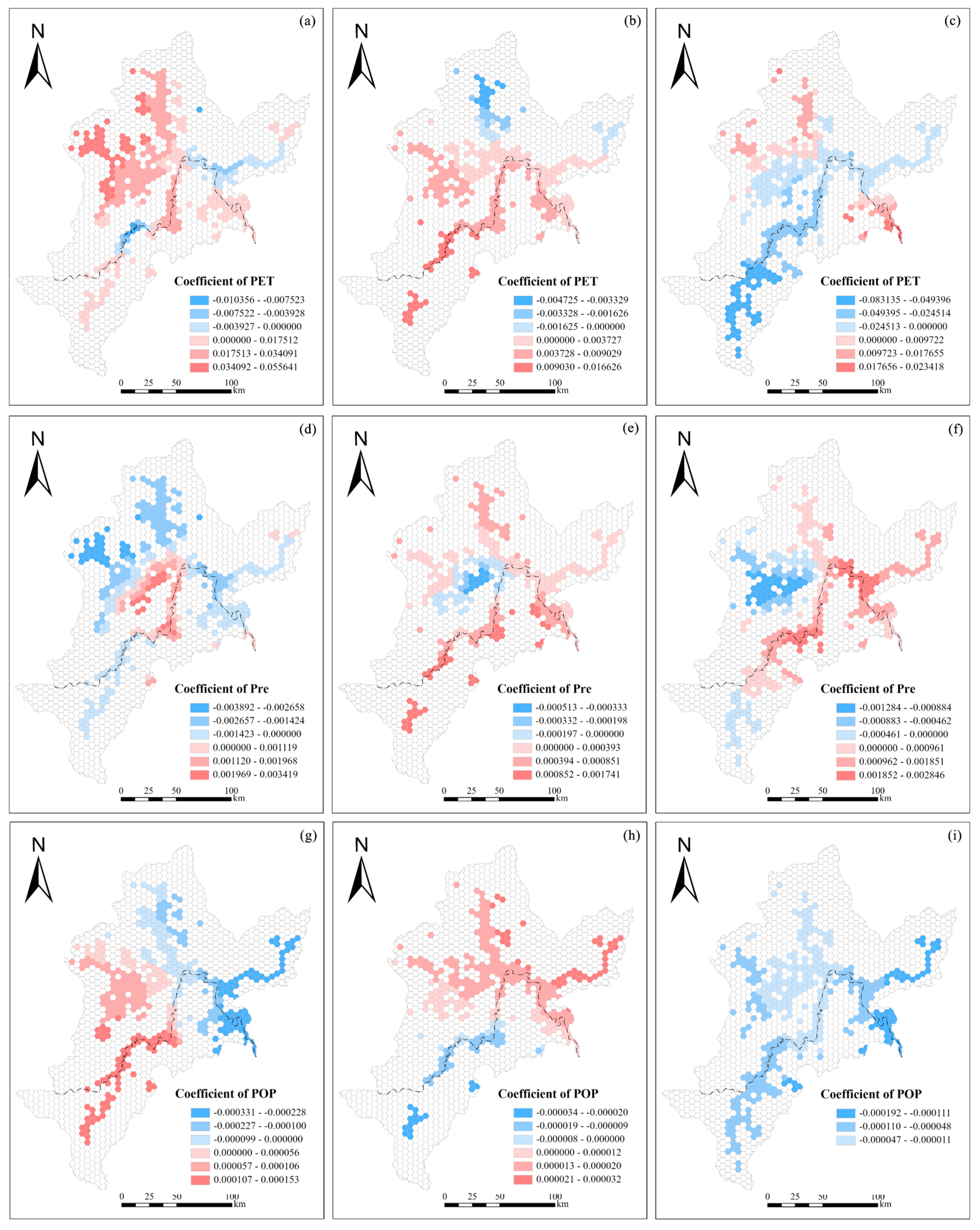
At the grid scale, the relationships between water area changes and factors such as potential evapotranspiration, precipitation, and population density reveal notable differences between China and North Korea.
Potential evapotranspiration (PET) shows varied impacts across the regions and months (Figure 11a–c). From June to July, most areas in the middle reaches of China exhibit a positive correlation with water area changes, whereas the downstream areas display a negative correlation. In contrast, both middle and downstream areas in North Korea predominantly show positive correlations. Moving into July to August, positive correlations are observed in the upper and downstream regions of China, while some middle areas show negative correlations. Conversely, in North Korea, positive correlations are widespread across most regions. By August to September, the upstream areas in both China and North Korea generally exhibit negative correlations, with some localized variations in other areas showing either positive or negative correlations.
Precipitation also affects water area changes differently across regions (Figure 11d–f). During June to July, negative correlations dominate the upstream areas in both China and North Korea, extending to most middle and downstream areas in China. However, the middle regions in North Korea show positive correlations. In the period from July to August, both upper and downstream areas in China generally show positive correlations, while some middle areas exhibit negative correlations. Across all regions in North Korea, positive correlations are observed during this period. By September, the middle regions in China display a mix of positive and negative correlations, while, in North Korea, the upstream areas show negative correlations, with positive correlations in the other regions.
Population density (POP) impacts water area changes with distinct patterns across time (Figure 11g–i). From June to July, positive correlations are seen in the upstream areas of both China and North Korea, while the downstream areas show negative correlations. During July to August, the upstream regions in both countries shift to negative correlations, whereas the middle and downstream areas exhibit positive correlations. By August to September, all areas in both China and North Korea show negative correlations, indicating a broad influence of population density on reducing the water area changes during this period.

4. Discussion

4.1. Spatiotemporal Characteristics and Emerging Hot Spot Analysis of Water in the Tumen River Basin

At the sub-watershed scale, the surface water area changes in the Tumen River Basin exhibit regional differences [52]. The upstream and midstream regions, characterized by high elevation, dense mountain ranges, fast-flowing rivers, and minimal human activity, show smaller and more stable surface water areas. These regions form cold spots and display a significant decreasing trend, predominantly influenced by natural conditions. In contrast, the downstream areas, benefiting from favorable hydrological conditions and significant influence from reservoirs and other hydraulic engineering projects, experience a rapid increase in surface water area [53]. This results in the formation of hot spots and a significant upward trend, indicating the crucial role of human activities in the expansion and management of surface water bodies [54]. At the grid scale, the data provide finer detail, enabling a more accurate reflection of local changes and avoiding the masking of details observed at the sub-watershed scale. Consequently, small hot spots and rising trends in the upstream regions are likely associated with artificial water bodies or water resource management practices, further highlighting the significant impact of human activities on surface water resources [55].

4.2. Analysis of the Driving Factors for Surface Water Area Changes Based on Random Forest Regression at Different Scales

In the comparative analysis of the sub-watershed and grid scales, the Random Forest model revealed significant differences in the primary driving factors for changes in the surface water area. At the sub-watershed scale, Pre was identified as the most important variable, followed by PET, POP, Paddy, and DEM [56]. Conversely, at the grid scale, PET emerged as the most crucial factor, followed by Pre, POP, Bare, and DEM [57]. This disparity reflects the varying influence of the geographical environment and human activities on surface water area changes at different scales.
At the sub-watershed scale, precipitation directly affects surface runoff and water body replenishment. Population density and wetlands are closely related to water resource utilization, significantly impacting changes in the surface water area [58]. At the grid scale, potential evapotranspiration plays a more substantial role in influencing the evaporation process of water bodies, and the impact of bare land highlights the effect of land use changes on the surface water area. Elevation, on the other hand, reflects the topographical constraints on water body distribution [59]. Moreover, the analysis at different scales demonstrates a common trend in the influence of precipitation and potential evapotranspiration on surface water area changes. Precipitation promotes an increase in surface water area within a low to moderate range, but the rate of increase slows after reaching a certain level. Potential evapotranspiration results in smaller water bodies at low levels, but as it increases, the surface water area expands. Population density also shows a consistent pattern: larger surface water areas are observed at low population densities. However, as the population density increases, human activities lead to changes in land use, affecting the surface water area. Once the population density reaches a certain threshold, changes in the surface water area stabilize. The effects of bare land and wetlands on the surface water area vary: an increase in the proportion of bare land leads to a decrease in the surface water area, reflecting the impact of urbanization. Wetlands, on the other hand, help regulate changes in the surface water area. A higher proportion of wetlands aids in maintaining the soil moisture and groundwater levels, reducing water evaporation and loss [60].

4.3. Analysis of the Driving Factors for Surface Water Area Changes Based on GWR

4.3.1. Comparative Analysis of the Driving Factors for Surface Water Area Changes in Different Countries

Regarding precipitation, the upstream regions of China and North Korea exhibit a negative correlation in June to July, which might be due to the rising river levels in these areas caused by rainfall, leading to a reduction in surface water area. Conversely, the midstream region of North Korea shows a positive correlation during the same period, possibly indicating that moderate precipitation positively impacts the increase in surface water area.
In terms of potential evapotranspiration, the changes in surface water area in China and North Korea show some similarities, but differences are also evident. For instance, the upstream region of North Korea exhibits a negative correlation in June to July, whereas China’s upstream region shows a positive correlation. This disparity could be attributed to differences in topography and climatic conditions. North Korea’s upstream region is predominantly characterized by steep mountainous terrain (Figure 1). The steep slopes lead to rapid runoff and reduced water retention, which can decrease the surface water area during periods of high evapotranspiration. Additionally, the mountainous regions may have microclimates that differ from the surrounding areas, further influencing the local hydrology. In contrast, China’s upstream region consists mainly of gentle plains (Figure 1). These plains facilitate greater water retention and slower runoff, maintaining the surface water area even when the potential evapotranspiration is high.
The relationship between population density and changes in the surface water area in the Tumen River Basin exhibits complex, yet consistent patterns across China and North Korea. Throughout different months, both countries show similar trends in how the population density correlates with the surface water area. For example, from June to July, higher population densities in upstream regions correspond with increases in the surface water, suggesting effective water retention and management. Meanwhile, downstream areas show a negative correlation, likely due to intensified water usage reducing the surface water availability. This observation echoes similar findings from other studies on transboundary basins, emphasizing the importance of considering socio-economic factors in water resource management [61].

4.3.2. Comparative Analysis of the Driving Factors for Surface Water Area Changes at Different Scales

At the sub-watershed scale, the relationship between changes in the surface water area and factors such as precipitation, potential evapotranspiration, and population density is more evident and complex. The influence of topography, climate, and land use on surface water area changes is more pronounced at this scale, potentially leading to regional differences.
At the grid scale, although relationships between the surface water area, precipitation, potential evapotranspiration, and population density still exist, they are likely to be more ambiguous and less distinct compared to the sub-watershed scale. The larger data granularity at the grid scale may not capture the subtle impacts of the geographical environment and human activities on surface water area changes, resulting in relatively weaker and more irregular relationships.

4.4. Strengths and Limitations of the Research Methods

This study leverages the robust computational capabilities of GEE along with remote sensing data from Landsat 8 and Sentinel-1 to analyze surface water area changes in the Tumen River Basin from 2015 to 2023. The research methods offer several strengths. First, GEE provides substantial computational power and data storage, enabling the efficient processing of large-scale remote sensing data. Second, employing methods such as Emerging Hot Spot Analysis, Random Forest Regression, and GWR allows us to uncover the spatiotemporal trends and driving mechanisms of water area changes from multiple perspectives and at various scales.
However, this study also has some limitations. First, although GEE excels in data processing and analysis, its reliance on internet connectivity and cloud computing resources may limit its applicability in certain research environments or scenarios. Second, the spatial and temporal resolutions of remote sensing data can affect the accuracy of the results, particularly in areas with complex terrain or significant climate variability. Additionally, while various statistical methods and models were employed, each has its assumptions and applicable conditions that may influence the results. Lastly, transboundary basin studies involve data and policies from multiple countries, and the consistency and accessibility of data can impact the comprehensiveness and accuracy of the study results.
Despite these limitations, this study provides important insights into the spatiotemporal dynamics of water resources in the Tumen River Basin and offers a reference framework for future research. Future studies could improve data acquisition and processing methods, incorporate more ground observation data, and enhance the accuracy and reliability of the analysis.

5. Conclusions

This study utilized remote sensing data from Landsat 8 and Sentinel-1, processed through Google Earth Engine (GEE), to rapidly and accurately extract the surface water area in the Tumen River Basin from 2015 to 2023. By employing Emerging Hot Spot Analysis, Random Forest Regression, and Geographically Weighted Regression (GWR), the spatiotemporal evolution trends and driving mechanisms of water area changes at different scales were revealed. The results indicate that GEE performed exceptionally well in extracting water areas, with an accuracy ranging from 95.75% to 98.25%. The surface water area in the Tumen River Basin showed an overall increasing trend, significantly peaking during the 2016 flood event. Upstream regions primarily formed cold spots influenced by natural conditions, whereas downstream regions developed hot spots driven by human activities. Precipitation, potential evaporation, and population density were identified as the main drivers of water area changes. There was notable spatial and temporal heterogeneity in the impact of these drivers across different countries and scales. Notably, the relationship between the population density and surface water area changes in the Tumen River Basin shows consistent patterns across both China and North Korea, though the specific impacts vary by region and month.
These insights underscore the importance of tailored management strategies for different regions within the basin. Upstream areas require conservation efforts focused on preserving the natural conditions, whereas the downstream regions benefit from the robust regulation and management of artificial water bodies. Furthermore, the study emphasizes the critical need for enhanced monitoring and cooperative management across national borders to address extreme climate events effectively.

Author Contributions

Conceptualization, R.J. and D.W.; methodology, R.J. and D.Q.; software, D.W.; validation, R.J. and D.W.; formal analysis, D.W.; investigation, D.W.; resources, R.J. and D.W.; data curation, D.Q. and D.W.; writing—original draft preparation, D.W.; writing—review and editing, R.J.; visualization, D.W.; supervision, R.J.; project administration, R.J.; funding acquisition, R.J. All authors have read and agreed to the published version of the manuscript.

Funding

This research was funded by the National Natural Science Foundation of China (41830643) and the Jilin Provincial Science and Technology Department Project (20210101106JC and 20200403030SF).

Data Availability Statement

The raw data supporting the conclusions of this article will be made available by the authors upon request.

Conflicts of Interest

The authors declare no conflicts of interest.

References

  1. Beven, K.; Cloke, H. Comment on: Hyperresolution global land surface modeling: Meeting a grand challenge for monitoring Earth’s terrestrial water by Eric F Wood et al. Water Resour. Res. 2012, 48, W01801. [Google Scholar] [CrossRef]
  2. Cosgrove, W.J.; Loucks, D.P. Water management: Current and future challenges and research directions. Water Resour. Res. 2015, 51, 4823–4839. [Google Scholar] [CrossRef]
  3. Yang, D.; Yang, Y.; Xia, J. Hydrological cycle and water resources in a changing world: A review. Geogr. Sustain. 2021, 2, 115–122. [Google Scholar] [CrossRef]
  4. Scanlon, B.R.; Fakhreddine, S.; Rateb, A.; de Graaf, I.; Famiglietti, J.; Gleeson, T.; Grafton, R.Q.; Jobbagy, E.; Kebede, S.; Kolusu, S.R.; et al. Global water resources and the role of groundwater in a resilient water future. Nat. Rev. Earth Environ. 2023, 4, 87–101. [Google Scholar] [CrossRef]
  5. Wang, Z.; Guo, J.; Ling, H.; Han, F.; Kong, Z.; Wang, W. Function zoning based on spatial and temporal changes in quantity and quality of ecosystem services under enhanced management of water resources in arid basins. Ecol. Indic. 2022, 137, 108725. [Google Scholar] [CrossRef]
  6. Mishra, R.K. Fresh water availability and its global challenge. Br. J. Multidiscip. Adv. Stud. 2023, 4, 1–78. [Google Scholar] [CrossRef]
  7. Lv, H.; Yang, L.; Zhou, J.; Zhang, X.; Wu, W.; Li, Y.; Jiang, D. Water resource synergy management in response to climate change in China: From the perspective of urban metabolism. Resour. Conserv. Recycl. 2020, 163, 105095. [Google Scholar] [CrossRef]
  8. Vila-Traver, J.; Aguilera, E.; Infante-Amate, J.; de Molina, M.G. Climate change and industrialization as the main drivers of Spanish agriculture water stress. Sci. Total Environ. 2021, 760, 143399. [Google Scholar] [CrossRef]
  9. Chen, H.; Liu, H.; Chen, X.; Qiao, Y. Analysis on impacts of hydro-climatic changes and human activities on available water changes in Central Asia. Sci. Total Environ. 2020, 737, 139779. [Google Scholar] [CrossRef] [PubMed]
  10. Duan, W.; Maskey, S.; Chaffe, P.L.; Luo, P.; He, B.; Wu, Y.; Hou, J. Recent advancement in remote sensing technology for hydrology analysis and water resources management. Remote Sens. 2021, 13, 1097. [Google Scholar] [CrossRef]
  11. Zhang, G.; Wang, M.; Zhang, T.; Chen, F. Progress in remote sensing monitoring of lake area, water level, and volume changes on the Tibetan Plateau. Natl. Remote Sens. Bull. 2022, 26, 115–125. [Google Scholar] [CrossRef]
  12. Liu, H. Application and Outlook of Remote Sensing Technology in Water Environment Monitoring. Highlights Sci. Eng. Technol. 2023, 69, 174–181. [Google Scholar] [CrossRef]
  13. Dehkordi, A.T.; Zoej, M.J.V.; Ghasemi, H.; Jafari, M.; Mehran, A. Monitoring long-term spatiotemporal changes in iran surface waters using landsat imagery. Remote Sens. 2022, 14, 4491. [Google Scholar] [CrossRef]
  14. Li, Y.; Niu, Z.; Xu, Z.; Yan, X. Construction of high spatial-temporal water body dataset in China based on Sentinel-1 archives and GEE. Remote Sens. 2020, 12, 2413. [Google Scholar] [CrossRef]
  15. Zhou, S.; Kan, P.; Silbernagel, J.; Jin, J. Application of image segmentation in surface water extraction of freshwater lakes using radar data. ISPRS Int. J. Geo-Inf. 2020, 9, 424. [Google Scholar] [CrossRef]
  16. Sekertekin, A. A Survey on global thresholding methods for mapping open water body using Sentinel-2 satellite imagery and normalized difference water index. Arch. Comput. Methods Eng. 2021, 28, 1335–1347. [Google Scholar] [CrossRef]
  17. Hu, Y.; Zhang, L.; Chen, B.; Zuo, J. An Object-Based Approach to Extract Aquaculture Ponds with 10-Meter Resolution Sentinel-2 Images: A Case Study of Wenchang City in Hainan Province. Remote Sens. 2024, 16, 1217. [Google Scholar] [CrossRef]
  18. Guo, Y.; Feng, C.; Xu, W.; Liu, Y.; Su, D.; Qi, C.; Dong, Z. Water-land classification for single-wavelength airborne LiDAR bathymetry based on waveform feature statistics and point cloud neighborhood analysis. Int. J. Appl. Earth Obs. Geoinf. 2023, 118, 103268. [Google Scholar] [CrossRef]
  19. Murray, N.J.; Phinn, S.R.; DeWitt, M.; Ferrari, R.; Johnston, R.; Lyons, M.B.; Clinton, N.; Thau, D.; Fuller, R.A. The global distribution and trajectory of tidal flats. Nature 2019, 565, 222–225. [Google Scholar] [CrossRef]
  20. Li, P.; Zhang, Y.; Liang, C.; Wang, H.; Li, Z. High spatiotemporal resolution river networks map** on catchment scale using satellite remote sensing imagery and DEM data. Geophys. Res. Lett. 2024, 51, 2023GL107956. [Google Scholar] [CrossRef]
  21. Qiu, Z.; Li, J.; Wang, Y.; Niu, Y.; Qian, H. Automatic Extraction Method of Landslide Based on Digital Elevation Model and Digital Orthophoto Map Data Combined in Complex Terrain. Appl. Sci. 2024, 14, 2771. [Google Scholar] [CrossRef]
  22. Du, Q.; Li, G.; Chen, D.; Qi, S.; Zhou, Y.; Wang, F.; Cao, Y. Extracting water body data based on SDWI and threshold segmentation: A case study in permafrost area surrounding Salt Lake in Hoh Xil, Qinghai-Tibet Plateau, China. Res. Cold Arid. Reg. 2023, 15, 202–209. [Google Scholar] [CrossRef]
  23. Han, C.; Jia, C.; Sun, Y. Remote Sensing Monitoring and Disaster Assessment of Flood Based on Sentinel-1B Sar Data. In Proceedings of the IGARSS 2022—2022 IEEE International Geoscience and Remote Sensing Symposium, Kuala Lumpur, Malaysia, 17–22 July 2022. [Google Scholar]
  24. Tian, P.; Liu, Y.; Li, J.; Pu, R.; Cao, L.; Zhang, H.; Ai, S.; Yang, Y. Mapping coastal aquaculture ponds of China using Sentinel SAR images in 2020 and google earth engine. Remote Sens. 2022, 14, 5372. [Google Scholar] [CrossRef]
  25. Li, H.; Xu, Z.; Zhou, Y.; He, X.; He, M. Flood Monitoring Using Sentinel-1 SAR for Agricultural Disaster Assessment in Poyang Lake Region. Remote Sens. 2023, 15, 5247. [Google Scholar] [CrossRef]
  26. Liu, C.; Xu, J.; Xu, K.; Yu, J. Mapping large-scale aquaculture ponds in Jiangsu Province, China: An automatic extraction framework based on Sentinel-1 time-series imagery. Aquaculture 2024, 581, 740441. [Google Scholar] [CrossRef]
  27. Pekel, J.-F.; Vancutsem, C.; Bastin, L.; Clerici, M.; Vanbogaert, E.; Bartholomé, E.; Defourny, P. A near real-time water surface detection method based on HSV transformation of MODIS multi-spectral time series data. Remote Sens. Environ. 2014, 140, 704–716. [Google Scholar] [CrossRef]
  28. Papa, F.; Prigent, C.; Aires, F.; Jimenez, C.; Rossow, W.B.; Matthews, E. Interannual variability of surface water extent at the global scale, 1993–2004. J. Geophys. Res. Atmos. 2010, 115, D12111. [Google Scholar] [CrossRef]
  29. Zou, Z.; Xiao, X.; Dong, J.; Qin, Y.; Doughty, R.B.; Menarguez, M.A.; Zhang, G.; Wang, J. Divergent Trends of Open-Surface Water Body Area in the Contiguous United States from 1984 to 2016. Proc. Natl. Acad. Sci. USA 2018, 115, 3810–3815. [Google Scholar] [CrossRef] [PubMed]
  30. Bian, J.; Li, A.; Lei, G.; Zhang, Z.; Nan, X. Global high-resolution mountain green cover index mapping based on Landsat images and Google Earth Engine. ISPRS J. Photogramm. Remote Sens. 2020, 162, 63–76. [Google Scholar] [CrossRef]
  31. Zhang, X.; Liu, L.Y.; Wu, C.S.; Chen, X.D.; Gao, Y.; Xie, S.; Zhang, B. Development of a global 30 m impervious surface map using multisource and multitemporal remote sensing datasets with the Google Earth Engine platform. Earth Syst. Sci. Data 2020, 12, 1625–1648. [Google Scholar] [CrossRef]
  32. Pekel, J.-F.; Cottam, A.; Gorelick, N.; Belward, A.S. High-resolution mapping of global surface water and its long-term changes. Nature 2016, 540, 418–422. [Google Scholar] [CrossRef]
  33. Wang, Y.; Li, Z.; Zeng, C.; Xia, G.S.; Shen, H. An Urban Water Extraction Method Combining Deep Learning and Google Earth Engine. IEEE J. Sel. Top. Appl. Earth Obs. Remote Sens. 2020, 13, 769–782. [Google Scholar] [CrossRef]
  34. Chen, N.; Yu, L.; Zhang, X.; Shen, Y.; Zeng, L.; Hu, Q.; Niyogi, D. Mapping Paddy Rice Fields by Combining Multi-Temporal Vegetation Index and Synthetic Aperture Radar Remote Sensing Data Using Google Earth Engine Machine Learning Platform. Remote Sens. 2020, 12, 2992. [Google Scholar] [CrossRef]
  35. Greifeneder, F.; Notarnicola, C.; Wagner, W. A Machine Learning-Based Approach for Surface Soil Moisture Estimations with Google Earth Engine. Remote Sens. 2021, 13, 2099. [Google Scholar] [CrossRef]
  36. Yang, X.; Chen, Y.; Wang, J. Combined use of Sentinel-2 and Landsat 8 to monitor water surface area dynamics using Google Earth Engine. Remote Sens. Lett. 2020, 11, 687–696. [Google Scholar] [CrossRef]
  37. Schaller, N.; Sillmann, J.; Müller, M.; Haarsma, R.; Hazeleger, W.; Hegdahl, T.J.; Kelder, T.; van den Oord, G.; Weerts, A.; Whan, K. The role of spatial and temporal model resolution in a flood event storyline approach in western Norway. Weather Clim. Extrem. 2020, 29, 100259. [Google Scholar] [CrossRef]
  38. Tao, S.; Fang, J.; Zhao, X.; Zhao, S.; Shen, H.; Hu, H.; Tang, Z.; Wang, Z.; Guo, Q. Rapid loss of lakes on the Mongolian Plateau. Proc. Natl. Acad. Sci. USA 2015, 112, 2281–2286. [Google Scholar] [CrossRef] [PubMed]
  39. Ji, L.; Gong, P.; Wang, J.; Shi, J.; Zhu, Z. Construction of the 500-m resolution daily global surface water change database (2001–2016). Water Resour. Res. 2018, 54, 10270–10292. [Google Scholar] [CrossRef]
  40. Gao, C.; Cheng, D.; Iqbal, J.; Yao, S. Spatiotemporal change analysis and prediction of the great yellow river region (GYRR) land cover and the relationship analysis with mountain hazards. Land 2023, 12, 340. [Google Scholar] [CrossRef]
  41. Milanović, S.; Marković, N.; Pamučar, D.; Gigović, L.; Kostić, P.; Milanović, S.D. Forest fire probability mapping in eastern Serbia: Logistic regression versus random forest method. Forests 2020, 12, 5. [Google Scholar] [CrossRef]
  42. Zhou, Y.; Dong, J.; Xiao, X.; Liu, R.; Zou, Z.; Zhao, G.; Ge, Q. Continuous monitoring of lake dynamics on the Mongolian Plateau using all available Landsat imagery and Google Earth Engine. Sci. Total Environ. 2019, 689, 366–380. [Google Scholar] [CrossRef] [PubMed]
  43. Li, L.; Su, H.; Du, Q.; Wu, T. A novel surface water index using local background information for long term and large-scale Landsat images. ISPRS J. Photogramm. Remote Sens. 2021, 172, 59–78. [Google Scholar] [CrossRef]
  44. Gao, B.-C. NDWI—A normalized difference water index for remote sensing of vegetation liquid water from space. Remote Sens. Environ. 1996, 58, 257–266. [Google Scholar] [CrossRef]
  45. Xu, X.; Xu, S.; Jin, L.; Song, E. Characteristic analysis of Otsu threshold and its applications. Pattern Recognit. Lett. 2011, 32, 956–961. [Google Scholar] [CrossRef]
  46. Acharya, T.D.; Subedi, A.; Lee, D.H. Evaluation of water indices for surface water extraction in a Landsat 8 scene of nepal. Sensors 2018, 18, 2580. [Google Scholar] [CrossRef] [PubMed]
  47. Huang, W.; DeVries, B.; Huang, C.; Lang, M.W.; Jones, J.W.; Creed, I.F.; Carroll, M.L. Automated extraction of surface water extent from Sentinel-1 data. Remote Sens. 2018, 10, 797. [Google Scholar] [CrossRef]
  48. Liu, Y.; Jin, R.; Zhu, W. Conversion of Natural Wetland to Farmland in the Tumen River Basin: Human and Environmental Factors. Remote Sens. 2021, 13, 3498. [Google Scholar] [CrossRef]
  49. Purwanto, P.; Utaya, S.; Handoyo, B.; Bachri, S.; Astuti, I.S.; Utomo, K.S.B.; Aldianto, Y.E. Spatiotemporal analysis of COVID-19 spread with emerging hotspot analysis and space–time cube models in East Java, Indonesia. ISPRS Int. J. Geo-Inf. 2021, 10, 133. [Google Scholar] [CrossRef]
  50. Svetnik, V.; Liaw, A.; Tong, C.; Culberson, J.C.; Sheridan, R.P.; Feuston, B.P. Random forest: A classification and regression Tool for compound classification and QSAR modeling. J. Chem. Inf. Comput. Sci. 2003, 43, 1947–1958. [Google Scholar] [CrossRef]
  51. Brunsdon, C.; Fotheringham, S.; Charlton, M. Geographically weighted regression. J. R. Stat. Soc. Ser. D 1998, 47, 431–443. [Google Scholar] [CrossRef]
  52. Chen, L.; Zhang, G.; Xu, Y.J.; Chen, S.; Wu, Y.; Gao, Z.; Yu, H. Human Activities and Climate Variability Affecting Inland Water Surface Area in a High Latitude River Basin. Water 2020, 12, 382. [Google Scholar] [CrossRef]
  53. Habersack, H.; Hein, T.; Stanica, A.; Liska, I.; Mair, R.; Jäger, E.; Hauer, C.; Bradley, C. Challenges of river basin management: Current status of, and prospects for, the River Danube from a river engineering perspective. Sci. Total Environ. 2016, 543, 828–845. [Google Scholar] [CrossRef]
  54. Yuan, R.; Li, Z.; Guo, S. Health risks of shallow groundwater in the five basins of Shanxi, China: Geographical, geological and human activity roles. Environ. Pollut. 2023, 316, 120524. [Google Scholar] [CrossRef] [PubMed]
  55. Jin, T.; Zhang, X.; Wang, T.; Liang, J.; Ma, W.; Xie, J. Spatiotemporal impacts of climate change and human activities on blue and green water resources in northwest river basins of China. Ecol. Indic. 2024, 160, 111823. [Google Scholar] [CrossRef]
  56. Wei, C.; Dong, X.; Ma, Y.; Leng, M.; Zhao, W.; Zhang, C.; Yu, D.; Su, B. Relationships between Landscape Patterns and Hydrological Processes in the Subtropical Monsoon Climate Zone of Southeastern China. Remote Sens. 2023, 15, 2290. [Google Scholar] [CrossRef]
  57. Liu, C.; Zou, L.; Xia, J.; Chen, X.; Zuo, L.; Yu, J. Spatiotemporal Heterogeneity of Water Conservation Function and Its Driving Factors in the Upper Yangtze River Basin. Remote Sens. 2023, 15, 5246. [Google Scholar] [CrossRef]
  58. Liu, Y.; Xie, X.; Tursun, A.; Wang, Y.; Jiang, F.; Zheng, B. Surface water expansion due to increasing water demand on the Loess Plateau. J. Hydrol. Reg. Stud. 2023, 49, 101485. [Google Scholar] [CrossRef]
  59. Lu, H.; Zhao, R.; Zhao, L.; Lyu, B.; Wang, J.; Zhang, L. A contrarian growth: The spatiotemporal dynamics of open-surface water bodies on the northern slope of Kunlun Mountains. Ecol. Indic. 2023, 157, 111249. [Google Scholar] [CrossRef]
  60. Gautam, P.K.; Chandra, S.; Henry, P.K. Monitoring of the Groundwater Level using GRACE with GLDAS Satellite Data in Ganga Plain, India to Understand the Challenges of Groundwater, Depletion, Problems, and Strategies for Mitigation. Environ. Challenges 2024, 15, 100874. [Google Scholar] [CrossRef]
  61. Hussein, H.; Grandi, M. Contexts matter: A hydropolitical analysis of Blue Nile and Yarmouk River basins. Soc. Water Stud. Arab. Reg. 2015, 159, 159–176. [Google Scholar]
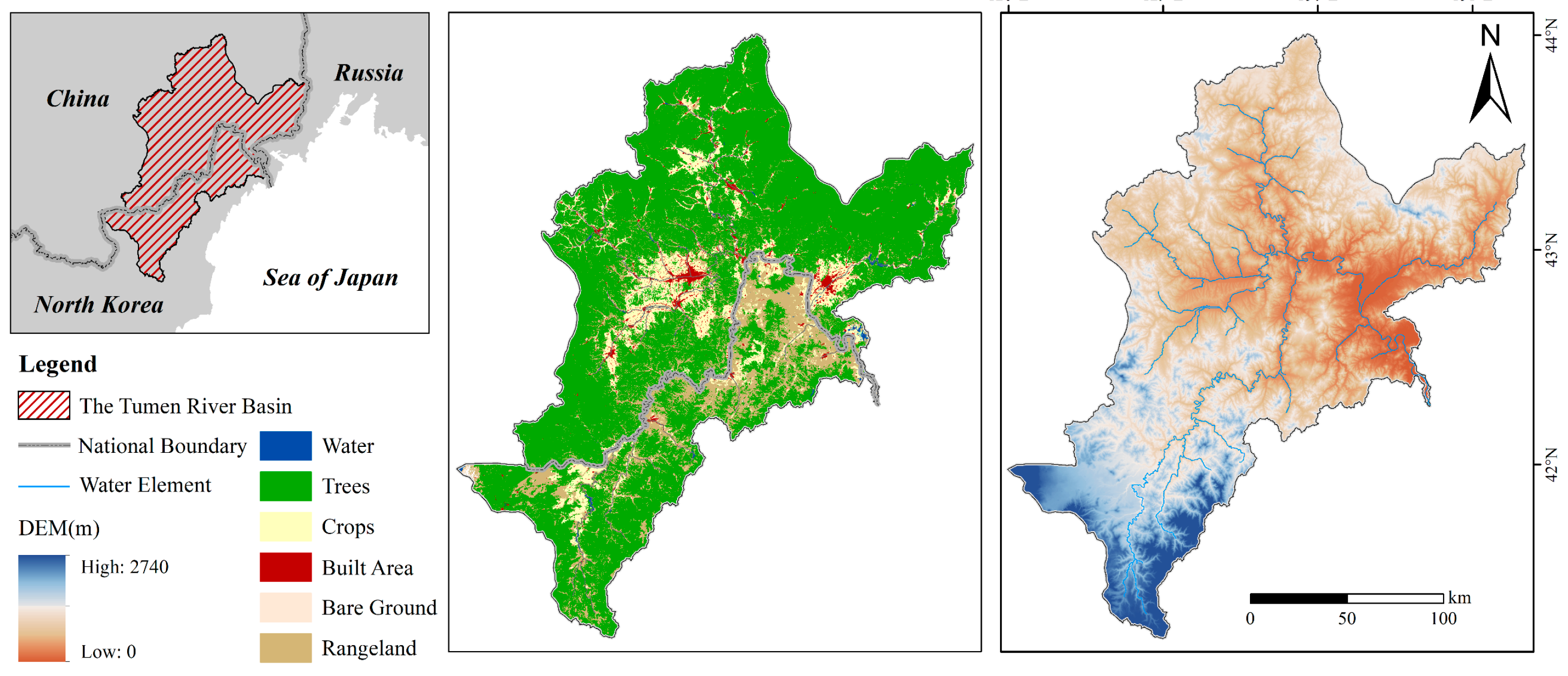
Figure 1. Schematic map of the study area.
Water 16 02185 g001
Figure 2. Technical roadmap.
Water 16 02185 g002
Figure 3. Schematic diagram of different scale divisions. (a) Sub-basins. (b) Grid cells.
Water 16 02185 g003
Figure 4. Changes in the water area in the Tumen River Basin (2015–2023).
Water 16 02185 g004
Figure 5. (a) Hot–cold spot patterns, (b) hot–cold spot trends, and (c) water area hot–cold spot 3D in the Tumen River Basin at the sub-basins scale.
Water 16 02185 g005
Figure 6. (a) Hot–cold spot patterns, (b) hot–cold spot trends, and (c) water area hot–cold spot 3D in the Tumen River Basin at the grid scale.
Water 16 02185 g006
Figure 7. Relative importance of drivers of water area change at the (a) sub-basin and (b) grid scales.
Water 16 02185 g007
Figure 8. Partial dependence plots for the driving factors of water area changes at the sub-basin scale.
Water 16 02185 g008
Figure 9. Partial dependence plots for the driving factors of water area changes at the grid scale.
Water 16 02185 g009
Figure 10. Spatial distribution of the regression coefficients for different driving factors in relation to surface water area changes in 2016 at the sub-basin scale. (a) Precipitation from June to July. (b) Precipitation from July to August. (c) Precipitation from August to September. (d) Potential evapotranspiration from June to July. (e) Potential evapotranspiration from July to August. (f) Potential evapotranspiration from August to September. (g) Population density from June to July. (h) Population density from July to August. (i) Population density from August to September.
Water 16 02185 g010
Figure 11. Spatial distribution of the regression coefficients for different driving factors in relation to surface water area changes in 2016 at the grid scale. (a) Potential evapotranspiration from June to July. (b) Potential evapotranspiration from July to August. (c) Potential evapotranspiration from August to September. (d) Precipitation from June to July. (e) Precipitation from July to August. (f) Precipitation from August to September. (g) Population density from June to July. (h) Population density from July to August. (i) Population density from August to September.
Water 16 02185 g011
Table 1. Data sources.
DateTemporal ResolutionData Sources
Sentinel-1 SARJune to September 2015–2023GEE (https://earthengine.google.com/, accessed on 10 June 2024)
Landsat 8June to August 2016GEE (https://earthengine.google.com/, accessed on 10 June 2024)
PrecipitationJune to August 2015–2023NOAA (https://www.psl.noaa.gov/data/gridded/index.html, accessed on 10 June 2024)
Potential EvaporationJune to August 2015–2023University of BRISTOL (Hourly potential evapotranspiration (hPET) at 0.1 degs grid resolution for the global land surface from 1981–present—Datasets—data.bris)
DEM/NASA and DLR (https://earthexplorer.usgs.gov/, accessed on 10 June 2024)
Hydrological System/GRDC (https://grdc.bafg.de/GRDC/EN/02_srvcs/22_gslrs/221_MRB/riverbasins_node.html, accessed on 10 June 2024)
Land Use Types2017–2022Impact Observatory (https://livingatlas.arcgis.com/landcoverexplorer/#mapCenter=28.77098%2C41.26723%2C11&mode=step&timeExtent=2017%2C2023&year=2023, accessed on 10 June 2024)
Population Density2015–2020WorldPop (https://hub.worldpop.org/geodata/listing?id=76, accessed on 10 June 2024)
Table 2. Confusion matrix for the accuracy assessment of water extraction results in August 2016.
ClassGround Truth PointsUser’s
Accuracy (%)
Producer’s
Accuracy (%)
WaterNon-WaterTotal
Water1991621599.5092.00
Non-Water118418592.5699.46
Total200200400
Note: Kappa coefficient is 0.92. Overall accuracy is 95.75%.
Table 3. Confusion matrix for the accuracy assessment of water extraction results in September 2023.
ClassGround Truth PointsUser’s
Accuracy (%)
Producer’s
Accuracy (%)
WaterNon-WaterTotal
Water197420198.50%98.00%
Non-Water319619998.01%98.49%
Total200200400
Note: Kappa coefficient is 0.97. Overall accuracy is 98.25%.
Table 4. Model mean squared error and R2 at different scales.
ScaleMean Squared ErrorR2
Sub-basin0.1310.819
Grid0.0270.853
Table 5. Multicollinearity test results of independent variables at different scales.
VariableVIF
Sub-Basin ScaleGrid Scale
June–JulyJuly–AugustAugust–SeptemberJune–JulyJuly–AugustAugust–September
PRE2.792.001.612.511.871.41
PET3.741.291.873.491.472.58
Trees1.931.311.931.361.391.38
Paddy23.0714.3336.2047.6047.0957.63
Bare2.061.802.031.661.611.61
Crops43.5742.4440.9441.3139.3746.75
Built6.816.906.636.146.716.58
Rangeland22.5519.7432.2240.5538.9048.12
POP4.562.243.213.032.953.04
DEM2.322.501.842.262.292.04
Slope3.444.903.404.284.824.23
Aspect4.185.234.731.081.091.11
River_dens1.501.531.801.261.422.14
Table 6. Model fit comparison at different scales.
ScaleModel
Parameter
June–JulyJuly–AugustAugust–September
OLSGWROLSGWROLSGWR
Sub-BasinAICc373.87356.70220.94209.56250.96245.37
R20.0750.3550.1200.4670.1070.300
Adjusted R20.0850.2160.1740.3080.1530.195
GridAICc207.22104.48164.37104.48–142.13–144.88
R20.0780.4910.1380.5810.1720.470
Adjusted R20.1240.3890.2440.4990.3200.366
Disclaimer/Publisher’s Note: The statements, opinions and data contained in all publications are solely those of the individual author(s) and contributor(s) and not of MDPI and/or the editor(s). MDPI and/or the editor(s) disclaim responsibility for any injury to people or property resulting from any ideas, methods, instructions or products referred to in the content.