Abstract
Hydrological modeling can be challenging due to significant data requirements and computational complexities. Hydrological models must be sufficiently complex to describe physical processes yet simple enough to use. This paper describes the development of a simplified watershed-scale input–output model to simulate runoff quantity and quality during a storm event. This work builds upon an existing semi-distributed rainfall–runoff model by adding calculations for pollutant concentrations based on simplified mass balance equations. The model was tested against various watershed examples of increasing complexity. The results show the change in peak flow and pollutant concentration in different areas of the watershed, demonstrating the model’s ability to account for the dynamics of runoff movement through the watershed. This paper advances watershed management by addressing data scarcity through the development of a simplified hydrological model that effectively incorporates spatial variability within a watershed while requiring minimal data input.
1. Introduction
Integrated Water Resource Management (IWRM) promotes the collaborative development of water, land, and resource management. The purpose of IWRM is to maximize economic and social benefits without compromising the ecosystem [1,2]. Implementing IWRM has many challenges due to the nonlinear and dynamic nature of water systems, as well as the presence of multiple and sometimes conflicting objectives. Additionally, water resource systems include many components, such as watersheds, rivers, groundwater, and reservoirs. Managing these systems is complex due to the need to integrate social, economic, environmental, and technical perspectives [3]. Therefore, IWRM requires Decision Support Systems (DSSs) to provide stakeholders and planners with the tools and information required for informed decision making. DSSs can be knowledge-based, GIS-based, use mathematical models, or rely on more complex decision support strategies [4]. Though many hydrological models have been developed and applied to different watershed management issues, several significant limitations remain. The challenges of hydrological modeling include large data requirements, limited spatial and temporal resolutions, and computational complexity. Planners and stakeholders need user-friendly models to simulate hydrological processes and help with optimal decision making regarding appropriate flood mitigation and runoff management measures. These models need to be both sufficiently complex to describe the physical processes occurring in the basin during the creation of surface runoff, and simple to use.
The rise in urbanization and the potential effects of climate change have increased the risk of floods and intensified surface degradation and nonpoint source (NPS) pollution [5,6]. Stormwater runoff primarily contributes to the pollution of streams and other water bodies [7]. The variability in pollutant concentrations during storm events significantly impacts the overall quality of urban stormwater [8]. Various factors contribute to the quality of stormwater runoff, firstly through the processes of buildup and wash-off. The buildup process assumes that during dry weather (when there is no rain), pollutants accumulate on the ground, and this buildup is dependent on land use. When rainfall occurs, a portion of these pollutants is carried and washed off in the formed runoff. The wash-off process can be influenced by rainfall intensity and is commonly modeled using empirical equations with a limited physical basis [9]. Furthermore, during the initial event, pollutants may be flushed out from storage areas in the landscape in a process called “first flush”. To prevent substantial pollutant loads from entering water bodies, the first flush phenomenon must be considered when designing stormwater control measures [8].
Subsequently, as the rainfall event progresses, the pollutant concentration in the runoff will be diluted, leading to a decrease in concentration due to the addition of water and the depletion of the pollutant’s sources. It is important to account for these processes as stormwater control measures designed to enhance water quality, like detention ponds, will cause different responses than measures intended for flood control [10]. Assessing the volume and strength of the first flush is crucial for guiding environmentally sustainable decisions in the design and management of stormwater control and treatment practices [8].
Various methods have been developed to account for water quality and quantity in urban and non-urban areas [9]. The soil and water assessment tool (SWAT) simulates the nutrient cycles of nitrogen and phosphorus as well as the degradation of pesticides based on soil composition and land use data. However, SWAT is a continuous long-term model unsuited for event-based calculations [11]. The stormwater management model (SWMM) is a physically-based hydrological model that simulates water quantity and quality for a single event or long-term continuous simulation and runoff transport in the drainage system. A SWMM models water quality based on the buildup and wash-off processes by simulating the buildup on surfaces, depending on the land use, and subsequent wash-off of pollutants, depending on rainfall intensity and duration. However, it is mainly designed to simulate an urban drainage system and has extensive data requirements [9]. Candido et al. (2022) conducted a review of existing basin-level models and DSSs for water allocation considering water quantity–quality management and sustainability. They found that though several models integrating water quantity–quality management have been developed, few integrate water quality with socioeconomic considerations. They underscore the importance of developing comprehensive yet simple-to-use models that address diverse challenges in water resource management [12].
This paper describes the development of a simplified runoff quantity and quality model through the addition of water quality equations to Diskin’s cell model, an existing rainfall–runoff model. Diskin et al. (1984) developed a semi-distributed routing model designed for hydrological simulation at the watershed scale. The model is semi-distributed, meaning it accounts for spatial variability within the watershed while maintaining a simplified representation of processes that allow for the simulation of spatially variable rainfall events. The watershed is divided into units of area represented by individual cells in the model. These cells are interconnected in a tree-like structure following the main drainage pattern of the watershed. The model distinguishes between rainfall excess inputs and channel inflow inputs to each cell. Rainfall excess refers to the portion of rainfall that contributes to surface runoff after infiltration and other losses, while channel inflow represents the flow entering a cell from upstream channels [13].
The boundaries of each cell are determined along the watershed lines of the main channels in the basin so that surface runoff crosses the cell boundaries at a small number of points. The advantage of the cell model is that physiographic features and factors can be expressed without the arduous work of determining the basin’s geomorphological structure and simultaneously simulating different distributions of hydrological processes that affect rainfall and surface runoff relationships [14].
Ostfeld and Pries (2002) used Diskin’s cell model to develop a GIS-based hydrological model to assess flow and contamination transport within the Lake Kinneret watershed in Israel, which they solved for the entire watershed in steady-state conditions [15]. Abrha and Ostfeld (2021) introduced a multi-compartment modeling approach to evaluate water quality in a water storage system. They developed compartmental models for both conservative and non-conservative materials in water storage systems. They used a basic mass balance equation to describe the concentrations of materials in each compartment and created different simplified differential equations for each type of compartment [16]. This paper builds upon these previous works by developing pollutant concentration equations that will allow each cell to compute the change in concentration during the rainfall event. Similar to Diskin’s model, we also divided concentration into two types, and similar to Abrha and Ostfeld (2021) [16], the concentration equation was based on simplified mass balance equations. We detail the full process of developing the equations, demonstrate the model’s performance for several example watersheds with varying degrees of complexity, and discuss potential applications.
2. Materials and Methods
2.1. Runoff Quantity Calculation
Diskin’s cell model, used to calculate runoff quantity, is a semi-distributed hydrological model in which the watershed is divided into cells, representing the subbasins in the watershed. Each cell is assumed to be hydrologically homogeneous, thus representing a lumped model within a semi-distributed framework. The model can also simulate interconnected watersheds by representing each watershed as a cell. In this model, each cell functions as a linear reservoir, with runoff determined by the amount of water stored within the cell. The watershed topography determines the subbasin boundaries and water movement dynamics between cells. Runoff flows from upstream cells to downstream cells according to the stream network. The model maintains mass balance, accounting for each cell’s inflows, outflows, and storage changes. All cells are interconnected in a tree-like structure based on the drainage pattern of the watershed. Each cell can have two types of inputs: (1) runoff resulting from excess rainfall and (2) runoff flowing from upstream cells. This categorization distinguishes between two types of cells: exterior cells, which only receive input from excess rainfall, and interior cells, which receive both excess rainfall and inflow from upstream cells [13]. Regardless of type, each cell in the model has the same structure, as detailed in Figure 1. The model input is uniformed rainfall intensities () for a storm event at regular time intervals (). The rainfall excess input to each cell is transformed into runoff by routing it through a pair of linear reservoirs ( and ) connected in series. Additionally, the channel inflow from upstream cells is routed through a linear channel and reservoir. In exterior cells, the channel inflow is zero, as they do not receive inflow from upstream cells.
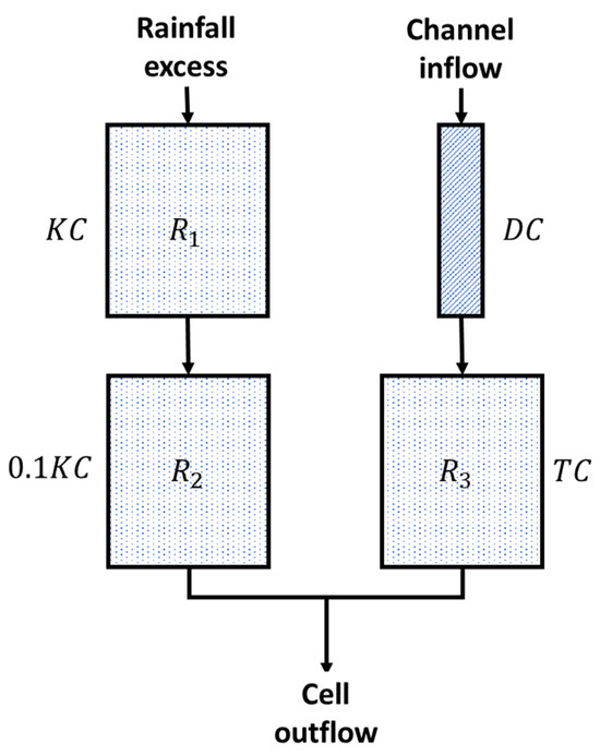
Figure 1.
The structure of a single-cell unit comprising two linear reservoirs ( and ), each with a reservoir constant a linear channel with a time delay constant , and a linear reservoir () with a reservoir constant . Adapted from Diskin et al. (1984) [13].
Reservoir and are represented by the linear reservoir constant , which is proportional to the square root of the area represented by the cell (Equation (1) adapted from [13]).
Assuming that the area of a cell is , the average size of the cells in the watershed is , and that the reservoir constant for this cell is . To keep the number of parameters to a minimum, the reservoir constant of the reservoir was arbitrarily taken to be 0.1 of the value of the constant for the reservoir .
The impulse response function for runoff from excess rainfall adapted from [13] is given in Equation (2), and runoff for each cell () is calculated using Equation (3).
Runoff from upstream flow from nearby cells is routed through a model consisting of a linear channel and a linear reservoir () in series (Figure 1). The upstream runoff input is first delayed by a time delay constant and then routed through the linear reservoir with a reservoir constant . To minimize the number of parameters these two constants are assumed to be proportional to the length of the channel length of each cell relative to the average channel length of all cells. Calculations of these variables were adapted from [13] and are presented in Equations (4) and (5).
Assuming that the channel length for each cell is , the average channel length of the cells in the watershed is , and and are channel flow time dilation factor and reservoir channel flow constant, respectively. Runoff from channel flow () can then be calculated using the impulse response function () shown in Equation (6), adapted from [13]. The complete calculation of channel flow is described in Equations (7) and (8).
2.2. Developing Water Quality Equations
To enhance Diskin’s cell model, which only calculates water quantity, we have developed equations that will work in tandem with Diskin’s model and compute water quality by calculating the accumulation and progression of pollutant concentration during a storm event. To maintain Diskin’s model’s semi-distributed nature, we have divided the pollutant concentration inputs to each cell into two types: (1) concentration accumulation in runoff formed due to excess rainfall and (2) concentration in runoff flowing from upstream cells.
Similarly to Abrha and Ostfeld (2021) [16], we describe the subbasin cells as inflow–outflow tanks, each with two compartments. The water quality in each compartment changes during the rainfall event due to runoff. In keeping with Diskin’s model, one compartment is filled with excess rainfall, and one is filled with flow from upstream cells. The pollutant is assumed to be a non-conservative material. Non-conservative materials are substances subject to changes in concentration due to biological, chemical, or physical processes. Nutrients like nitrogen and phosphorus are non-conservative, as are heavy metals and pesticides [17]. Monitoring the change in concentration of these materials during a rainfall event is crucial to assess water quality and understand the impact of human activities on water quality.
We started with basic equations for the conservation of volume and concentration, where the volume change is equal to inflow minus outflow (Equation (9)). The change in concentration is equal to the concentration of pollutants in the inflow minus the concentration in the outflow and a further loss of material depended on a first-order decay constant () shown in Equations (10) and (11).
Figure 2 depicts a system of two tanks. Each tank has two compartments: one is filled from excess rainfall and one from flow from a previous tank. These assumptions created simpler differential equations that can be solved by integration.
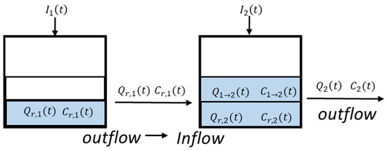
Figure 2.
Depiction of the two storage tanks system; each tank has two compartments.
Equations (12)–(19) detail the development of a concentration equation due to rainfall excess. Specifically, Equations (12)–(14) represent simplified versions of the conservation of volume and concentration equations (Equations (9)–(11)), assuming conditions of only outflow.
Combining Equations (12) and (14) results in Equation (15)
Equations (16)–(19) details the solving and integration process of Equation (15).
Equation (19) is the final concentration from the rainfall excess equation, where is the concentration from the rainfall excess entering cell and is the initial concentration of a pollutant in the ground.
Equations (20)–(27) detail the development of concentration from upstream cells. Since the pollutants in the compartment arrive due to runoff flowing from a previous cell, there are several assumptions: (1) the compartment has only inflow, (2) the decay constant () is equal to zero, and (3) and are equal to the runoff and concentration from an upstream cell, respectively. Equations (20)–(22) are the simplified versions of Equations (9)–(11), assuming conditions of only inflow.
Combining Equations (20) and (22) results in Equation (23)
Equations (24)–(27) detail the solving and integration process of Equation (23).
Equation (27) is the final equation for the concentration of the runoff flowing from an upstream cell, where is the concentration from an upstream cell entering cell . The combined concentration at the outlet of each cell is given in Equation (28).
Figure 3 gives a detailed illustration of runoff quantity and pollutant concentration inputs and outputs for a watershed example with two subbasins depicted as a two-cell model.
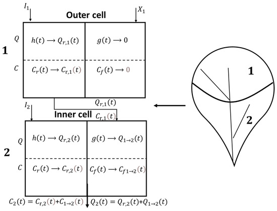
Figure 3.
Illustration of rainfall to runoff and pollutant concentration inputs and outputs for a watershed with two subbasins depicted as a two-cell model. Example watersheds description.
The model was examined for three different watershed networks with a rising level of complexity. We began with the two-cell watershed example shown in Figure 3. To test the model’s ability to simulate more complex systems, we then examined the model for a five-cell watershed example shown in Figure 4.
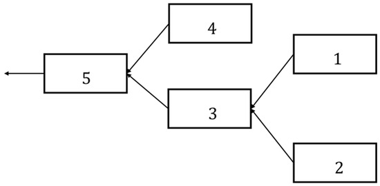
Figure 4.
Five-cell watershed example illustration.
For both simple examples, we used the same reservoir routing coefficient , linear channel length constant and channel routing coefficient . These are example values selected to ensure consistency with the scales observed in our 15-cell watershed example. The cell area and channel length parameters for these example watersheds are listed in Table 1.

Table 1.
Cell area and channel length data for the three example watersheds.
Finally, to illustrate the application of the model, we tested the model using data from the Bellebeek watershed, as originally described by Diskin et al. (1984) [13]. The Bellebeek watershed is located in Belgium and covers an area of with a main steam length of . Diskin selected the the Bellebeek watershed as a case study due to its multiple gauging stations. We chose the Bellebeek watershed as an example in our research to examine how our model, with the addition of concentration equations, behaves with an already tried and proven case.
The 15-cell example of the Bellebeek watershed is shown in Figure 5. Unless stated otherwise, all the parameters we used in this example were adapted from Diskin’s paper [13]. We used the reservoir routing coefficient , linear channel length constant and channel routing coefficient . For cell characteristics, not all cells area and channel length were listed in [13]. Since we are only interested in testing our model with a more complex watershed and not conducting calibration using real data, we used a mean value or an example value with a similar scale in the case of a missing value. A complete list of cell areas and channel lengths appears in Table 1.
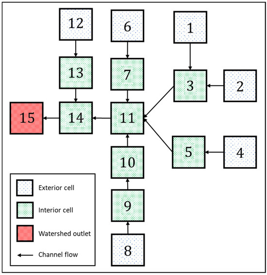
Figure 5.
Fifteen cells example (Bellebeek watershed) adapted from Diskin et al. (1984) [13].
The same rainfall intensity for the storm event was used for all three examples, as shown in Figure 6. The rainfall data, adapted from [15], were selected primarily to ensure consistency across all watershed examples. Utilizing the same rainfall data for all three watersheds allowed us to examine the model’s performance across watersheds with varying levels of complexity without the variability that differing rainfall events might introduce.
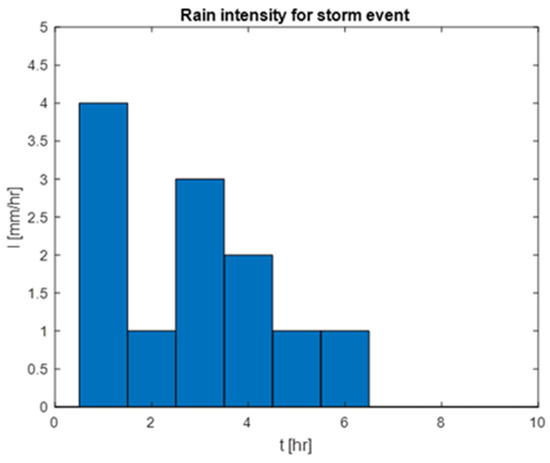
Figure 6.
Rainfall intensity for the storm event used for the three example watersheds.
We performed calculations for one example pollutant () with a and rate constant assumed for all cells. Ammonia () was selected as a representative pollutant because nitrogen nutrients, such as ammonia, are common in urban and agricultural runoff and have detrimental environmental effects, particularly on aquatic systems [18]. The initial concentration and rate constant were adapted from [15]. The model was developed in MATLAB version R2022a [19]. Detailed calculations for the 2-cell and 5-cell examples in Excel can be found in Supplementary Material S1, and the MATLAB code for all three examples can be found in Supplementary Materials S2–S4.
3. Results
To test the water quality and quantity model, we applied it to three watershed examples. Figure 7 presents the runoff flow and concentration for the two-cell example. Figure 7a,b shows the flow and concentration in cell 1, which is an exterior cell where runoff and concentration are formed due to excess rainfall. Figure 7c,d shows the results for the runoff and concentration in cell 2, which is an interior cell and the watershed outlet. In cell 2, there are two runoff and concentration inputs—excess rainfall and upstream cell (cell 1).
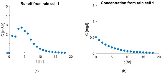
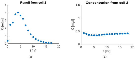
Figure 7.
Flow and concentration results for the two-cell watershed example, depicting: (a) runoff from Cell 1, (b) concentration in Cell 1, (c) runoff from Cell 2 (outlet), (d) concentration in Cell 2 (outlet).
As can be seen, the peak flow in cell 2 is higher than that in cell 1. The higher peak flow is because the runoff at the watershed outlet (cell 2) is the sum of the runoff from cell 1 and the runoff formed from excess rainfall in cell 2. In the concentration results (Figure 7b,c), the concentration starts high and slowly decreases as the storm event progresses, mimicking the first flush and dilution processes. Additionally, the concentration in cell 2 is higher than in cell 1 due to the concentration input from runoff from the upstream cell (cell 1) and the concentration forming from excess rainfall in cell 2.
Figure 8 presents flow and concentration results for the five-cell example, showing the results for cell 1 (Figure 8a,b), an exterior cell, and cell 5 (Figure 8c,d), an interior cell, and the watershed outlet. The same trend of a higher peak flow at the outlet compared to the exterior cells is observed in the five-cell example. This trend can be attributed to the accumulation of runoff throughout the watershed. Additionally, the concentration at the outlet is higher than in the exterior cells because downstream basins receive runoff from multiple upstream areas, each contributing its own load of pollutants. Therefore, as runoff flows from one basin to another, the concentration of pollutants can increase. Moreover, there is a slight rise in pollutant concentration immediately following the peak flow, which then decreases. This pattern aligns with the higher runoff volumes during peak flows, which carry larger loads of accumulated pollutants. After the peak flow, dilution occurs as more water enters the system without a corresponding increase in pollutant load.
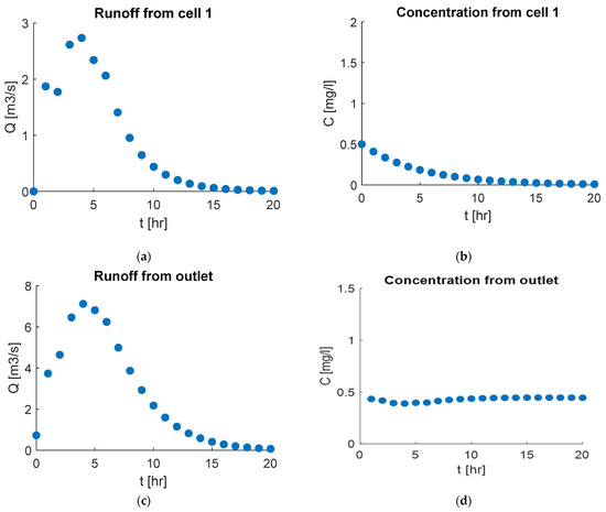
Figure 8.
Flow and concentration results for the five-cell watershed example, depicting: (a) runoff from Cell 1, (b) concentration in Cell 1, (c) runoff from Cell 5 (outlet), (d) concentration in Cell 5 (outlet).
Finally, Figure 9 shows the runoff hydrograph and concentration levels for the 15-cell example, including (1) cell 3 (Figure 9a,b), which is an interior cell receiving runoff and concentration inputs from two exterior cells (cells 1 and 2); (2) cell 11 (Figure 9c,d) which is an interior cell with inputs from four other interior cells (cells 3, 5, 7, and 10); and (3) the watershed outlet at cell 15 (Figure 9e,f). Here, we can observe that the peak flow is not only higher but also forms later the more we progress in the watershed due to a delay in the flow of runoff from cell to cell (the delay is determined from parameter ). As for concentration, the concentration of pollutants in cell 11, a downstream cell receiving runoff from multiple upstream basins, is higher compared to cell 3, which receives runoff from fewer basins. This pattern is due to the accumulation of runoff and associated pollutants, consistent with previous watershed examples. The concentrations in cell 11 and cell 15 (the watershed outlet) are nearly identical; this can be explained by the significant role that cell 11 plays in the watershed. As a major contributor of runoff and pollutants, cell 11 receives inputs from many upstream basins. This influx accumulates runoff and pollutants, which are then carried downstream to the outlet. This pattern highlights the importance of managing and monitoring key nodes within a watershed that significantly influence downstream water quality.
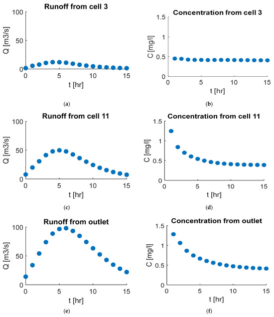
Figure 9.
Flow and concentration results for the 15-cell watershed example (Bellebeek watershed), depicting: (a) runoff from Cell 3, (b) concentration in Cell 3, (c) runoff from Cell 11, (d) concentration in Cell 11, (e) runoff from Cell 15 (outlet), (f) concentration in Cell 15 (outlet).
4. Discussion
Here, we present a simplified hydrological model that accounts for spatial variability within a watershed while requiring minimal data such as watershed topography, subbasin areas, and channel lengths. This model can be adapted to different watersheds and variables and could serve as a basis for the simulation of various optimization problems related to watershed management. Simulating peak flow for storm events is essential for watershed management because it allows for targeted flood management rather than reducing all runoff. Moreover, by simulating the peak flow and pollutant concentration in different areas of the watershed during a storm event, we can inform the targeted placement of flood and pollutant mitigation measures by identifying areas with the highest peak flow rates and pollutant concentrations and prioritizing locations for intervention where it will have the most significant impact on reducing flooding and pollutant loads. The model can also be adapted for combined watershed networks, where each watershed is represented as an individual cell. This adaptation allows for the simulation of pollutant dynamics across interconnected watersheds, enhancing its suitability for comprehensive stormwater management.
One potential use for the model is for the issue of IWRM, which integrates multidisciplinary approaches into a holistic water management strategy. Various countries have developed different water management methods and terminologies [6]. These more sustainable approaches often use nature-based solutions (NBSs) to increase infiltration and detain water. NBSs are measures inspired by and supported by nature and can provide environmental, social, and economic benefits. NBSs can provide an additional source for water provision, enhance water quality, and mitigate peak flow. Additionally, NBSs can improve ecosystem services through biodiversity rehabilitation and protection, improve public health, and provide areas for recreational activity [20]. The optimal placement of NBSs should be part of a regional-based strategy. However, a DSS regarding the optimal placement of NBSs require extensive data and expert input, which is not readily available for all areas. The model presented here uses simplified equations and minimal input data, making it especially suitable for NBS placement decisions. While the initial results presented here are promising and showcase the model’s simplicity and ability to simulate different types of watersheds, further research is needed to enhance the model’s applicability for watershed management. Future studies should prioritize calibration using observational data to enhance model accuracy. Calibration enables researchers to fine tune models to local conditions and validate the model assumptions and parameters against real-world measurements. Calibrating can be challenging, particularly in basins with limited data availability necessary for calibration. Researchers can employ several approaches to facilitate model calibration in regions with limited data availability. These methods include remote sensing data, in situ field measurements, and statistical techniques to generate data based on available information [21]. The model presented here is simple, with few parameters to calibrate, which could help facilitate the calibration process, especially in data-scarce areas.
Furthermore, addressing the placement of NBSs requires identifying and incorporating parameters that simulate their effects on the watershed, such as infiltration rates, pollutant removal, and flow attenuation. Lastly, the model should be integrated into an optimization framework to determine the optimal location and type of NBS or other flood mitigation measures within the watershed.
5. Conclusions
This paper details the construction of a hydrological water quantity and quality model by augmenting Diskin’s semi-distributed rainfall–runoff cell model with pollutant concentration equations derived from mass balance principles. The model’s performance was evaluated across various watershed scenarios, illustrating its ability to simulate peak flow and pollutant concentration dynamics during storm events. This hydrological model requires minimal data input and can be adjusted to simulate the effect of NBS or other flood and pollutant mitigation measures on the watershed. Despite some limitations, the research makes several noteworthy contributions to the field of watershed management and hydrological modeling by detailing the development of water quality equations and incorporating them into a semi-distributed input–output water quantity model, suggesting potential application for the model, and discussing future research.
Supplementary Materials
The following supporting information can be downloaded at: https://www.mdpi.com/article/10.3390/w16152072/s1, Spreadsheets S1: Cellmodel Two and Five Cells Examples; MATLAB code (PDF) S2: Example_2cell; MATLAB code (PDF) S3: Example_5cell; MATLAB code (PDF) S4: Example_15cell.
Author Contributions
Conceptualization, M.T.-m. and A.O.; Formal analysis, M.T.-m.; Methodology, M.T.-m.; Supervision, A.O.; Writing—original draft, M.T.-m.; Writing—review and editing, A.O. All authors have read and agreed to the published version of the manuscript.
Funding
This research received no external funding.
Data Availability Statement
Data is contained within the article or supplementary materials.
Conflicts of Interest
The authors declare no conflict of interest.
References
- GWP. Integrated Water Resources Management; Global Water Partnership. Technical Advisory Committee (TAC) Background paper No.4; Global Water Partnership: Stockholm, Sweden, 2000. [Google Scholar] [CrossRef]
- Hering, J.G.; Ingold, K.M. Water resources management: What should be integrated? Science 2012, 336, 1234–1235. [Google Scholar] [CrossRef] [PubMed]
- Ostfeld, A. Ant colony optimization for water resources systems analysis–review and challenges. In Ant Colony Optimization-Methods and Applications; IntechOpen Limited: London, UK, 2011. [Google Scholar]
- Le Page, M.; Fakir, Y.; Aouissi, J. Modeling for Integrated Water Resources Management in the Mediterranean Region. In Water Resources in the Mediterranean Region; Zribi, M., Brocca, L., Tramblay, Y., Molle, F., Eds.; Elsevier Inc.: Amsterdam, The Netherlands, 2020; Chapter 7; pp. 157–190. [Google Scholar] [CrossRef]
- Srivastava, P.; Hamlett, J.M.; Robillard, P.D.; Day, R.L. Watershed optimization of best management practices using AnnAGNPS and a genetic algorithm. Water Resour. Res. 2002, 38, 3-1–3-14. [Google Scholar] [CrossRef]
- Zhang, K.; Chui, T.F.M. A comprehensive review of spatial allocation of LID-BMP-GI practices: Strategies and optimization tools. Sci. Total Environ. 2018, 621, 915–929. [Google Scholar] [CrossRef] [PubMed]
- Jalali, P.; Rabotyagov, S. Science of the Total Environment Quantifying cumulative effectiveness of green stormwater infrastructure in improving water quality. Sci. Total Environ. 2020, 731, 138953. [Google Scholar] [CrossRef] [PubMed]
- Todeschini, S. Innovative and Reliable Assessment of Polluted Stormwater Runoff for Effective Stormwater Management. Water 2024, 16, 16. [Google Scholar] [CrossRef]
- Rossman, L.A.; Huber, W.C. Storm Water Management Model Reference Manual Volume III—Water Quality; US Environmental Protection Agency: Cincinnati, OH, USA, 2016.
- Jefferson, A.J.; Bhaskar, A.S.; Hopkins, K.G.; Fanelli, R.; Avellaneda, P.M.; McMillan, S.K. Stormwater management network effectiveness and implications for urban watershed function: A critical review. Hydrol. Process. 2017, 31, 4056–4080. [Google Scholar] [CrossRef]
- Neitsch, S.L.; Arnold, J.G.; Kiniry, J.R.; Williams, J.R. Soil and Water Assessment Tool Theoretical Documentation Version 2009; Technical Report 406; Texas Water Resources Institute, Texas A&M University: College Station, TX, USA, 2011. [Google Scholar]
- Candido, L.A.; Coelho, G.A.G.; de Moraes, M.M.G.A.; Florêncio, L. Review of Decision Support Systems and Allocation Models for Integrated Water Resources Management Focusing on Joint Water Quantity-Quality. J. Water Resour. Plan. Manag. 2022, 148, 03121001. [Google Scholar] [CrossRef]
- Diskin, M.H.; Wyseure, G.; Feyen, J. Application of a Cell Model to the Bellebeek Watershed. Hydrol. Res. 1984, 15, 25–38. [Google Scholar] [CrossRef]
- Milman, T. Calibration of Parameters of Cell Model for Rainfall Excess-Surface Runoff Relations. Master’s Thesis, Technion—Israel Institute of Technology, Haifa, Israel, 1989. [Google Scholar]
- Ostfeld, A.; Pries, A. Lake Kinneret watershed contamination transports—A GIS based hydrological model. Water Sci. Technol. 2002, 48, 63–70. [Google Scholar] [CrossRef]
- Abrha, B.; Ostfeld, A. Analytical Solutions to Conservative and Non-Conservative Water Quality Constituents in Water Distribution System Storage Tanks. Water 2021, 13, 3502. [Google Scholar] [CrossRef]
- Baker, M.A.; Webster, J.R. Conservative and Reactive Solute Dynamics. In Methods in Stream Ecology; Academic Press: Cambridge, MA, USA, 2017; pp. 129–146. [Google Scholar]
- Cheng, J.; Bi, J.; Gong, Y.; Cheng, X.; Yu, J.; Gan, H.; Wang, K. Processes of nitrogen removal from rainwater runoff in bioretention filters modified with ceramsite and activated carbon. Environ. Technol. 2023, 44, 3317–3330. [Google Scholar] [CrossRef]
- The MathWorks Inc. MATLAB Version: 9.12.0; The MathWorks Inc.: Natick, MA, USA, 2022; Available online: https://www.mathworks.com (accessed on 31 August 2023).
- Liu, L.; Dobson, B.; Mijic, A. Optimisation of urban-rural nature-based solutions for integrated catchment water management. J. Environ. Manag. 2023, 329, 117045. [Google Scholar] [CrossRef] [PubMed]
- Anand, V.; Oinam, B.; Srinivasan, R.; Wieprecht, S.; Singh, S.K. Enhancing hydrological model calibration through hybrid strategies in data-scarce regions. Hydrol. Process. 2024, 38, e15084. [Google Scholar] [CrossRef]
Disclaimer/Publisher’s Note: The statements, opinions and data contained in all publications are solely those of the individual author(s) and contributor(s) and not of MDPI and/or the editor(s). MDPI and/or the editor(s) disclaim responsibility for any injury to people or property resulting from any ideas, methods, instructions or products referred to in the content. |
© 2024 by the authors. Licensee MDPI, Basel, Switzerland. This article is an open access article distributed under the terms and conditions of the Creative Commons Attribution (CC BY) license (https://creativecommons.org/licenses/by/4.0/).