Abstract
The assessment of water quality assumes a position of utmost significance as it plays a critical role in upholding ecological balance and safeguarding the well-being of human populations. To achieve these goals, an in-depth consideration of water quality trends is essential, as it offers comprehension into the intricate interplay between various elements within aquatic ecosystems. As a consequence, the proposed work investigates the water quality trends specifically within the Valliyar sub-basin, which encompasses the geographical areas of Kattathurai, Colachal, Thuckalay, and Villukuri. The temporal scope of investigation spans from the year 2000 to 2018 using the dependent variable of water quality parameters with dependent variables of climate data. Recognizing the need for advanced methodologies to tackle the multifaceted nature of water quality dynamics, this research harnesses the power of pioneering machine learning techniques. Two notable approaches, the Radial Bias Function Neural Network (RBFNN) and the DenseNet-121-based Convolutional Neural Network (CNN), are brought into performance. The primary objective is to leverage these techniques to forecast water quality trends for the next twenty-two years. The effectiveness of various machine learning models in predicting water quality is evaluated using the following key performance metrics: the Mean-Square Error (MSE), Mean Absolute Percentage Error (MAPE) and Root-Mean-Square Error (RMSE). Notably, the DenseNet CNN model exhibits accurate prediction among the Artificial Neural Network (ANN), Support Vector Machine (SVM), and Deep Learning (DL) models. This research underscores the significance of machine learning techniques, with DenseNet CNN model emerging as a particularly promising tool in this domain.
1. Introduction
The combination of declining groundwater levels and the growing demands of population, urbanization, and human activities has led to significant global impacts in the groundwater. Groundwater, a vital and renewable resource, is under the constant threat of depletion in India [1,2,3,4]. Influencing the delicate balance of ecosystems underscores the fact that the quality of water plays a vital role in maintaining the equilibrium within ecosystems. Even small changes in water quality lead to the disruption of the intricate balance between different species and natural processes. Recognizing potential groundwater areas is the initial phase in effectively harnessing both groundwater and surface water resources. This requires understanding the movement of groundwater, which is influenced by various factors within a particular region [5].
The chemistry of heavy metals in aquatic environments is deeply influenced by key physicochemical parameters such as pH, temperature, salinity, electric conductivity, Total Dissolved Solids (TDSs), and turbidity, which collectively shape their solubility, speciation, and toxicity levels [6,7]. When toxic heavy metals exceed acceptable thresholds, water becomes unfit for drinking, industrial use, and agriculture, posing risks to human health and ecosystem integrity [8]. However, other significant pollutants also affect groundwater, including Volatile Organic Compounds (VOCs) and Polycyclic Aromatic Hydrocarbons (PAHs), which stem from industrial processes and significantly compromise water quality. VOCs, including trichloroethylene and benzene [9], along with PAHs from the incomplete combustion of carbon associated fuels [10], contribute towards the contamination through industrial and atmospheric deposition. Also, other pollutants from industries such as pharmaceutical residues and endocrine disruption compounds further contaminate the groundwater. But, in the proposed research work, there is no industrial activity near the assessment area, and the contamination is mainly due to agricultural practices, such as pesticides and fertilizers. Due to these persistent biogeochemical effects, ecological impacts, and its non-biodegradable nature, there is an urgent need for environmental management and regulation [11].
The assessment of water quality relies significantly on both physicochemical and microbiological parameters. In the realm of physicochemical properties, numerous parameters come into play, including pH, Electrical Conductivity (EC), TDS, chloride levels, turbidity, phosphate content, hardness, nitrate concentrations, and more [12,13]. Evaluating the suitability of drinking water involves comparing these parameters to established standards, as delineated by the Environmental Protection Agency (EPA) and World Health Organization (WHO) [14,15]. These standards serve as crucial benchmarks for determining the acceptability and safety of drinking water quality.
The demand for robust, dependable, precise, and adaptable prediction models has surged in response to the growing recognition of groundwater pollution concerns and the heightened interest in water quality assessment [16]. These models are expected to offer a precise depiction of the mechanisms behind water quality deterioration [17]. To tackle this challenge, researchers have embraced the concept of modelling both surface and underground water quality utilizing soft computing tools, particularly machine learning models, due to their reputation for reliability and accuracy [18,19]. Nevertheless, these models have encountered difficulties in generalizing and effectively handling the intricate and highly nonlinear relationships among the various modelling parameters.
Table 1 summarizes the existing machine learning methods used for groundwater quality assessment, along with their advantages, disadvantages, and limitations.

Table 1.
Existing classification techniques.
Hence it is important to select an advanced machine learning method for groundwater quality assessment based on the problem’s requirements and constraints. As a consequence, the proposed work establishes two different classifiers, the RBFNN and the DenseNet-121-based CNN technique, for more precise classification. Addressing the research gaps of existing studies, improved outcomes are attained by the proposed classifiers. The contributions of the research includes
- Assessment of long-term water quality trends in Valliyar sub-basin (2000–2018);
- Introduction of advanced machine learning techniques for water quality assessment;
- Forecasting of future water quality trends for next twenty-two years (2019–2040);
- Evaluation of machine learning models using key performance metrics;
- Identification of a highly effective model for water quality prediction;
- Emphasis on the significance of machine learning in understanding and forecasting water quality patterns.
2. Study Area
The Valliyar sub-basin is located in the Kanniyakumari district of Tamil Nadu, India. This region is known for its diverse natural landscapes, rich biodiversity, and its importance in environmental studies. As part of the proposed work, specific areas within the Valliyar Sub-basin were studied: Kattathurai (), Colachal (), Thuckalay (), and Villukuri (). These areas play a pivotal role in the proposed research, likely due to their distinctive characteristics, ecological significance, or potential impact on the overall ecosystem of the Valliyar Sub-basin. The latitude and longitude coordinates provided are specific to each area and are crucial for accurately pinpointing their geographical locations on a map, as seen in Figure 1. Transversely, all areas have human impacts on the quality of groundwater, due to residential developments in Thuckalay, and Villukuri, agricultural practices in Kattathurai and to coastal dynamics in Colachal. Understanding and analysing these areas’ geographical features, environmental conditions, and dynamics of chemical and physiochemical variables were essential components of the research work.
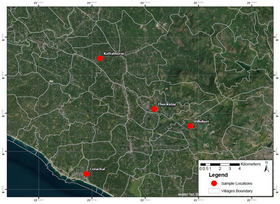
Figure 1.
Study areas of Valliyar sub-basins.
3. Proposed System Description
The proposed research highlights the critical significance of assessing groundwater quality. It emphasizes that this evaluation is crucial for maintaining ecological balance and safeguarding human populations’ well-being. By elucidating the critical nature of groundwater quality assessment, this research improves its attention on a specific geographical domain—: the Valliyar sub-basin, encompassing distinctive locales such as Kattathurai, Colachal, Thuckalay, and Villukuri—using advanced machine learning strategies. The architecture illustrated in Figure 2 demonstrates the overview of the proposed work.
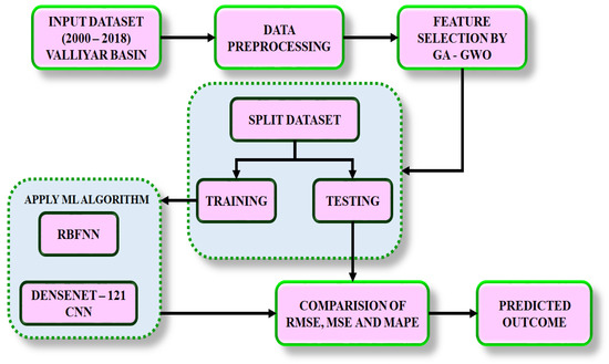
Figure 2.
Architecture of proposed system.
The initial stage involved data preparation, in which the proposed work utilized the dataset of Valliyar sub-basin of the year 2000–2018. The dataset consisted of both dependent and independent parameters. The dependent parameters included physicochemical parameters such as potential Hydrogen (pH), Electrical Conductivity (EC), Total Hardness (TH) and Total Dissolved Solids (TDSs), followed by chemical parameters such as Sodium (Na), Potassium (K), Sulphate (SO4), Calcium (Ca), Chloride (Cl), Magnesium (Mg) and Nitrate (NO3). These parameters were collectively utilized to indicate the quality and composition of water, while year, temperature, relative humidity, wind speed, pan evaporation and rainfall were the independent parameters. These variables were crucial as they influenced the water quality parameters under investigation. The dataset underwent a pre-processing stage, which focused on enhancing data quality by addressing missing values. Non-values or gaps within the dataset were systematically eliminated, ensuring that the dataset used for subsequent analyses was consistent, reliable, and free from incomplete or unreliable data points. After pre-processing, the Genetic Algorithm–Grey Wolf Optimization (GA-GWO) algorithm was employed for feature selection. All relevant independent variables were retained through this process, thus refining the dataset for accurate analysis. After selection of features, the classification stage was proceeded with using the RBFNN and DenseNet-121 CNN to predict relationships between independent and dependent variables. The effectiveness of a learning model was established through assessing its performance using MATLAB version-R2021aby various execution measures with diverse evaluation metrics including MSE, RMSE and MAPE, which were analysed individually for each area. Furthermore, the proposed work foreshows the future concentrations of crucial minerals over the year 2019–2040.
4. Modelling of Proposed System
4.1. Data Preparation and Preprocessing
Data preparation is the fundamental initial step in any data analysis. In the proposed research, on forecasting groundwater quality trends, this process involved systematically preparing the raw data for meaningful analysis. This entailed collecting data from the Valliyar sub-basin that provide information on water quality parameters such as pH, EC, TH, TDS, Na, K, SO4, Ca, Cl, Mg and NO3 as well as factors like temperature, humidity, wind speed, evaporation and rainfall from the years 2000–2018. Collecting the data from the Tamil Nadu Public Works Department, often dispersed across various sources, into a consolidated dataset is vital to ensure comprehensive coverage. Additionally, organizing the data into a structured format, typically a tabular arrangement with rows representing observations and columns representing different parameters facilitated subsequent analysis. Through diligent data preparation, the basis for deriving significant insights into the groundwater quality trends within the Valliyar sub-basin over the specified time period was accomplished.
Data pre-processing, the subsequent step after data preparation, is a critical phase that focuses on refining the prepared dataset to ensure its suitability for analysis and modelling. In the context of this research on forecasting groundwater quality trends, data pre-processing involved a series of strategic actions. These encompass addressing outliers and anomalies within both dependent and independent parameters. By identifying extreme values and either transforming or removing them, the dataset was made more robust against excessive influence from outliers.
After pre-processing, the extraction of optimal features from dataset was performed in this research, utilizing a hybrid algorithm combining GA and GWO.
4.2. Feature Selection by GA-GWO
After preparation of data, we created an initial population of feature subsets using binary encoding, where each bit represents the selection status of a feature (0: not selected, 1: selected). The size of the population and the length of each binary string correspond to the number of features in the dataset. Subsequently, we defined a fitness function that quantifies the quality of each feature subset. This function evaluates the performance of a machine learning model using selected features.
Then, we applied Genetic Algorithm operations to evolve the population:
Selection: choose parent feature subsets based on their fitness values.
Crossover: create offspring subsets through crossover operations, combining features from parent subsets.
Mutation: introduce random mutations to maintain diversity.
Replacement: replace less fit parent subsets with better-performing offspring to form the next generation.
Consequently, we incorporated GWO to further refine the feature selections, by converting the fittest feature subsets from GA phase into initial solutions (wolves) for GWO. We updated the positions of ( wolves) around using GWO equations, simulating cooperative hunting behaviour to enhance feature selections.
The encircling operation of wolves is given by given by and , coefficient vectors as and , and the updated position is denoted as :
where and denotes co-efficient vectors.
From the above equation, the updated position of is indicated as and .
Iterative optimization was performed in alternate between the GA and GWO phases, as seen in Figure 3, enabling them to collaboratively optimize the feature subsets. GA explored a wide search space, while GWO fine-tuned selections based on fitness values.
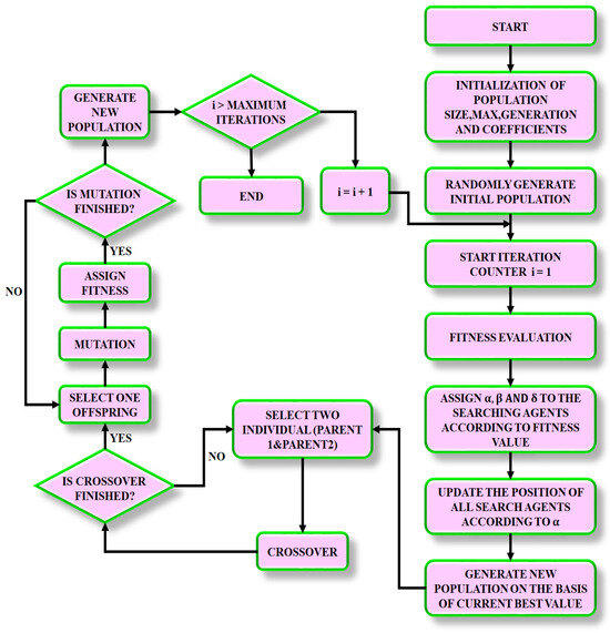
Figure 3.
Flowchart for GA-GWO-based feature selection.
Finally, convergence was monitored to identify when the optimization process stabilized. When the predefined termination criteria were met, the process was stopped. Alternatively, if the criteria were not satisfied, the fitness evaluation was repeated, and the subsequent iteration was executed. The input parameters of the GA-GWO approach were given by population size set to 100, allowing a maximum iteration of 50, crossover probability of 0.7 and mutation probability at 0.1. This ensured moderate chance of random variations in selecting optimal features. As a result, features such as year, temperature, relative humidity, wind speed, and pan evaporation were extracted. The final stage of the process was classification, in which the proposed work utilized two distinct classification strategies, which were proceeded as follows.
4.3. Classification by RBFNN
The RBFNN, a type of feed-forward neural network with a single hidden layer, was built upon the kernel method concept. RBF employs radial basis functions as feature maps, which are real-valued functions determined solely by the distances between input vectors and a fixed vector. This model is well suited for the task of regression that involves complex non-linear relationships, and commonly environmental data. In the proposed work, its response to localized input features makes it sensitive to changes in variables for analysing water quality. An example is the Gaussian function , with as a fixed vector and as a free parameter. Interestingly, the RBF network design shows that varying radial basis functions in the hidden layer has minimal impact on performance, allowing focus on Gaussian functions. These functions are widely preferred due to their effectiveness, serving as prominent feature maps in this context. The specification of RBFNN is listed in Table 2.

Table 2.
Specification of RBFNN.
The RBF network structure is illustrated in Figure 4. Inputs are n-dimensional real vectors In the hidden layer, each is calculated using a Gaussian function determined by parameters and . In the end, output is expressed as a linear representation with weights . To introduce further flexibility, a bias is incorporated, modifying the output to .
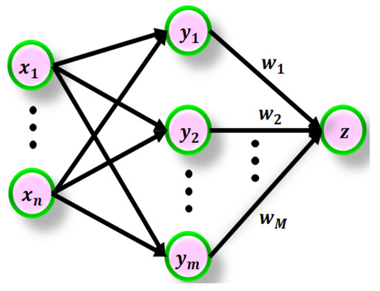
Figure 4.
Architecture of RBFNN [26].
Training an RBF network involves two main steps. Initially, we parameterized the Gaussian functions, and specified centres and width .
Centres can be training samples or, more effectively, can be identified using the K-means algorithm. Here, the number of weights can be notably fewer than training samples. The second step encompasses weight determination through solving a least-square problem.
For instance, consider a binary classification scenario in which there are training samples; is a discrete value, and suggests data points in the -dimensional space:
When the centres correspond to the training samples, the feature mapping is established as follows.
is the network’s ability to map input data in the n-dimensional space to output data in the M-dimensional space, and it is learned during the training of the network to perform classification.
On choosing , the weights are obtained by solving the least-square problem:
From Equation (6), denotes the weight vector of the dimension , loss function, which is as close as possible to the actual target values .
The training process required to solve the aforementioned least-square problem consumes a significant amount of time when executed on a classical computer. To mitigate this issue, the recursive least-square method is frequently employed. This approach serves to alleviate the computational burden associated with calculating matrix inversion. In the classification phase, we fed the pertinent data (features) into the pre-trained RBFNN. We computed the activation for each hidden layer neuron using Gaussian functions, considering input data and corresponding centres. We computed the weighted sum of hidden layer outputs using established weights. Finally, we employed suitable activation function (like linear activation) to derive the ultimate output. The resulting output signified the anticipated groundwater quality trend or pertinent classification outcome. Subsequently, we measured the precision of RBFNN’s forecasts by employing performance metrics, including MSE, MAPE, and RMSE.
4.4. Classification by DenseNet-121-Based CNN
The DenseNet-121 model is a CNN-based architecture designed for classification tasks. The proposed DenseNet-121model encompasses four main layers, illustrated in Figure 5. In the proposed work, it was designed to be particularly effective for handling high-dimensional and complex datasets, such as those encountered in water quality monitoring. In the CNN model, the process begins with an input data which undergoes filter application to generate a feature map. The layer produces feature maps like from subsequent layers, as elaborated in Equation (7):
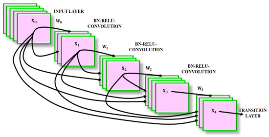
Figure 5.
Weighted DenseNet-121 CNN model [27].
From above expression, the concatenated set of feature maps is represented as which emerges from the layers spanning from . To enhance non-linearity, an activation function like Rectified Linear Unit (ReLU) is employed at pooling layer during feature map input. The function generates mapping features at level, subsequently followed by the layer, which is assessed using Equation (8).
In Equation (8), represents the total input layer channels, and the hyperparameter influences the network’s growth rate. Each layer integrates feature maps with distinct states. Neuron weights are computed through dot products, while input data computations consider the volume relationship.
A summary of layers comprising the DenseNet-121 Model is listed in Table 3. It outlines the proposed model, which began with a convolutional layer accompanying a max pooling layer to minimize the size of input. The interconnection of dense block and reduced the dimensionality size of the data. The final global average and softmax layer generated the classified output.

Table 3.
Details of layers in DenseNet-121 CNN model.
Verification of neuron activation correctness relies on ReLU layers. The input layer is initialized with random weights denoted as , yielding resultant features. Here, , where signifies set of integers.The output values obtained are used to train weights across transition layers. ReLU maintains input data, while pooling layer reduces feature noise. Higher-level features are determined from Fully Connected (FC) layer outputs. Dense Net 121, part of deep CNN model, comprises 5 convolutional layers and 13 weight layers. It encompasses 4 FC layers and 2 Dense Net layers. Dropout regularization in the FC layer with an activation function is conducted. Activation functions are fed to convolutional layers, as expressed in Equation (9).
In Equation (9), signifies the output layer denoted as , represents the base value, and is referred to as the filter connection associated with feature map, considering level feature maps and level features. signifies output layer containing features. The model’s capability to eliminate unnecessary features effectively addresses the issue of overfitting.
Equations (10)–(12) possess the capability to construct feature maps through a transverse slice filter approach, effectively eliminating irrelevant features and mitigating overfitting challenges. In Equations (11) and (12), represents the parameters of a neural network, altering data transformations denoted as acquired from the filter. Additional layers, ReLU and FC, are depicted as presented in Equations (13) and (14):
where signifies the ReLU layer, the output layer is denoted as , and represents the FC layer, followed by convolutional layers that evaluate activation. DenseNet is applied for feature reuse, a key concept enhancing compact versions. Feature propagation’s intensity has led to a reduced parameter count, thereby accelerating model enhancement. DenseNet exhibits seamless interconnectivity between layers, facilitating direct connections among them. The DenseNet-121 architecture leverages pre-trained weights, emphasizing dense connections in the feed-forward network. Consequently, the DenseNet model outperforms alternative network architectures. The DenseNet-121 CNN model, with its dense connections and feature reuse, revolutionizes water quality assessment. Its compact design and pre-trained weights sustain its prediction, while the RMSE, MSE, and MAPE metrics validate its precision.
5. Results and Discussion
In the context of the proposed work, the model’s validation was based on RMSE, MSE and MAPE. The prediction was performed using classifiers such as RBFNN and the DenseNet 121-based CNN model and the outcomes were contrasted with other existing classification topologies. MSE and RMSE quantified the squared differences between the predicted and actual values, providing significance into model reliability. By dealing with larger errors, it ensured accurate predictions for the effective management of water quality. Also, these metrics were simple, with the same units as the predicted variable, making it straightforward for prediction errors. Additionally, the monitoring of MSE and RMSE resulted in enhanced predictive performance in predicting the quality of groundwater. Table 4 illustrates the parameters involved in the work, including both dependent and independent variables. A lot of research has elucidated that temperature, evaporation, and rainfall all impact groundwater quality. However, in the proposed improvements, temperature, wind speed, humidity, and pan evaporation—all of which are positively correlated with evaporation and soil temperature—have an impact on the quality of groundwater.

Table 4.
Factors in analysis.
Based on the dependent and independent variable, error performance measures were evaluated for the areas Kattathurai, Colachal, Thuckalay, and Villukuri of Valliyar Sub-basin. The correlation matrix for all four areas are depicted in Figure 6, Figure 7, Figure 8 and Figure 9. The figures define var1-pH, var2-EC, var3-Na, var4-K, var5-SO4, var6-TH, var7-Ca, var8-Cl, var9-Mg, var10-NO3, and var11-TDS. Similarly, var12-var17 specifies the independent variable in the order year, temperature, relative humidity, wind speed, pan evaporation and rainfall.
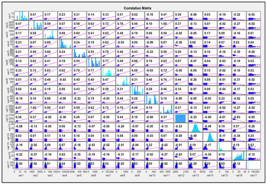
Figure 6.
Correlation matrix for Kattathurai.
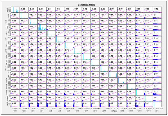
Figure 7.
Correlation matrix for Colachal.
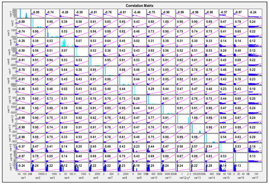
Figure 8.
Correlation matrix for Thuckalay.
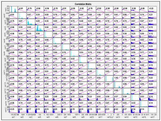
Figure 9.
Correlation matrix for Villukuri.
The correlation results between dependent and independent variables in Kattathurai are displayed in Figure 6. This correlation matrix mainly provides insights about the relationships between the water quality parameters (var1 to var11) and the independent variables (var12 to var17). Strong correlations (above +0.75) suggest that the related variables have a very significant linear relationship. In the context of water quality parameters, strong correlations indicate direct chemical relationships influencing these parameters. Moderate correlations (0.50–0.75) suggest a substantial but less overwhelming relationship than strong correlations. This reflects a significant but not exclusive linkage between the parameters. Weak correlations (0.30–0.50) suggest a mild relationship, which is not as compelling as moderate or strong correlations. Here, var6 (TH) has strong correlations with var7 (Ca), which reaffirms the fact that calcium is a major contributor to water hardness. Similarly, var11 (Solids, TDS) is also observed to have a strong correlation with var2 (EC) and var8 (Cl). Moreover, EC also has strong positive correlations with Cl, reinforcing the concept that ions are principal contributors to the conductivity of the water.
The correlation results between dependent and independent variables in Colachal are visually presented in Figure 7. The correlation matrix for Colachal reveals insightful relationships between various water quality parameters and climatic factors. Notably, pH is negatively correlated with most of the components, suggesting that water acidity has an inverse relationship with these substances. EC exhibits strong positive correlations with a multitude of dissolved ions such as Na, TH, Ca, Cl, Mg, Nitrate, and TDS. These strong relationships underscore EC as a key indicator of ionic activity in water. Sodium’s strong positive correlation with K, Sulphate, Cl, Mg, and TDS suggest similar behaviours of these ions in the aquatic system. Additionally, strong correlations between sulphate, TH, Ca, and Cl point to the presence of sulphate minerals that significantly influence the water’s physicochemical properties. The correlation of TH with several ions, as well as an apparent increase over time as suggested by its correlation with the year, highlights its role in water quality dynamics. Ca and Mg, essential for determining water hardness, showed strong correlations with Cl, Nitrate, and TDS, indicating their significant contributions to the mineral content of water. Chloride’s correlation with environmental factors such as Year, Temperature, and Relative Humidity implies its fluctuation with climatic conditions, affecting water salinity. Magnesium and Nitrate are not only intertwined with each other but also show a combined influence on TDS levels. Intriguingly, TDSs correlate strongly with temporal and environmental variables, hinting at the substantial impact of climatic changes on dissolved solids in water. Year, Temperature, Relative Humidity, and Pan Evaporation interrelate strongly, suggesting that these environmental measures are closely linked, reflecting broader climatic trends. Contrastingly, Rainfall does not exhibit a significant linear relationship with any of the studied parameters.
The correlations between dependent and independent variables in Thuckalay are graphically represented in Figure 8. The negative correlations observed with several variables suggest that an increase in pH is associated with a decrease in certain groundwater quality parameters, and vice versa. The strong negative correlation, particularly with variables that include ionic substances, indicates their solubility is affected by pH changes. EC stands out with strong positive correlations across a spectrum of ions, highlighting its utility as an indicator of the ionic content in groundwater. Sodium and potassium also share positive relationships with other ions, pointing to their significance in the groundwater’s overall ionic balance. TH correlates strongly with the presence of calcium and magnesium, affirming their roles in contributing to water hardness. These relationships are essential in understanding the mineral composition of groundwater and its overall quality. Furthermore, TDS exhibits positive correlations with numerous ions, reflecting the combined effect of various substances dissolved in the water. The independent variables, representing environmental influences like temperature and rainfall, show varied correlation strengths with the physicochemical properties, indicating that factors like climate play a differentiated role in determining groundwater quality. For instance, the lesser correlation with rainfall point is due to dilution effects or the introduction of new substances through precipitation.
The correlation matrix for the area Villukuri with dependent and independent variables is presented in Figure 9, revealing intricate relationships within the dataset. In Villukuri, the correlation matrix reveals a distinct pattern of strong positive correlations among various ionic constituents and key groundwater quality indicators such as EC and TDS, signifying that these ions are significant contributors to the overall mineral content of the groundwater. High negative correlations with pH suggest an inverse relationship with certain ionic concentrations. Notably, the matrix shows varying degrees of correlations between groundwater quality parameters and environmental factors, indicating the influence of external conditions on groundwater characteristics.
Each of these areas has distinct geographical characteristics, with Kattathurai as agricultural land, Colachal as a coastal area, and Thuckalay and Villukuri as residential areas. In the case of Kattathurai, the strong correlation between TH and Ca [28] indicates that agricultural activities, which often involve the use of calcium-containing compounds, significantly impact water hardness. The strong correlation between TDS and EC, along with Cl, suggests that agricultural runoff, which is rich in soluble salts, influences the water quality [29,30]. Weak to moderate correlations between independent variables like temperature, relative humidity, and wind speed with water quality parameters imply that while climatic factors do influence water quality, their impact is overshadowed by agricultural practices [31]. In case of Colachal, the strong positive correlation of EC with various ions (Na, TH, Ca, Cl, Mg, and ) reflects the significant influence of seawater intrusion and salinity on water quality, a common issue in coastal areas [32]. The negative correlation of pH with most components suggests that the water tends to become more acidic as the ionic concentration increases, possibly due to the dissolution of in seawater [33]. Strong correlations between the year and several parameters, including EC, indicate that water quality is undergoing changes over time, due to increased coastal activities, urbanization, and climatic changes affecting salinity [34]. In the case of Thuckalay, the strong negative correlations observed with pH and several variables indicate that domestic wastewater discharge, which is acidic, significantly impacts groundwater quality [35]. EC’s strong positive correlations across a spectrum of ions highlight the influence of domestic sewage, which contributes various ions to groundwater. The correlation between the year and parameters such as EC suggests a worsening trend in water quality over time, mainly due to increased residential density and insufficient wastewater management practices [36]. Similar to Thuckalay, strong negative correlations with pH and positive correlations with EC and various ions suggest the impact of urban runoff and domestic wastewater on water quality in Villukuri [37,38]. The consistent pattern across residential areas highlights the need for better wastewater treatment and urban planning to mitigate these impacts. The weak correlations between climatic factors and water quality parameters indicate that, although climate plays a role [39,40], the primary drivers of water quality changes in Villukuri are related to urbanization and residential activities [41,42].
Across all areas, the findings underscore the significant impact of human activities—agricultural practices in Kattathurai, coastal dynamics in Colachal and the residential developments in Thuckalay, and Villukuri—on groundwater quality. Climatic factors, while influential, play a secondary role to these anthropogenic factors. This analysis highlights the critical need for integrated water quality management strategies that consider both human and climatic influences to safeguard groundwater resources in these diverse geographical settings.
5.1. Mean-Square Error Measures
The analysis of MSE for physiochemical variables (such as pH, EC, Na, SO4, TH, Ca, Cl, Mg, NO3, and TDS) in different areas (Kattathurai, Colachal, Thuckalay, and Villukuri) of Valliyar Sub-basin with factors including year, temperature, humidity, wind speed, evaporation and rainfall using RBFNN and DenseNet-121 CNN is illustrated in Figure 10. The discussion shows that pH attains the lowest MSE, which is a measure of acidity or alkalinity of a solution that is commonly used to indicate water quality. The pH attained using RBFNN for Kattathurai was 0.0039, 0.0053 for Colachal, 0.0055 for Thuckalay and 0.0052 for Villukuri. However, on comparison, improved results were attained using the DenseNet-121 CNN classifier, where the MSE of pH for Kattathurai was 0.0019, and was 0.0022 for Colachal, 0.0019 for Thuckalay and 0.0018 for Villukuri. The analysis demonstrates that both classifiers provide improved results in predicting pH compared to the original data. The DenseNet-121 CNN classifier appeared to perform better in terms of lower MSE values for all areas compared to the RBFNN classifier. Among all the cases, Kattathurai appears to have the lowest MSE values for both classifiers, indicating that the predictions for pH.
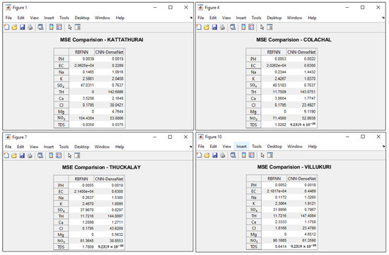
Figure 10.
MSE comparison.
5.2. Root-Mean-Square Error Measures
Figure 11 show cases comparative study involving the RBFNN and DenseNet-121 CNN to predict groundwater quality within the Valliyar sub-basin. The evaluation was based on the RMSE, which measured the water quality predictions. The analysis placed emphasis on variables including pH, EC, Na, SO4, TH, Ca, Cl, Mg, NO3, and TDS, with independent factors such as year, rainfall, temperature, humidity, wind speed, temperature and evaporation, with the RBFNN and DenseNet-121 CNN classifiers leading to a reduction in RMSE. In particular, pH shows reduced error performance, which signifies the acidity or alkalinity of a solution. A reduction in RMSE was observed for pH predictions; notably, for the specific location of Kattathurai, the RBFNN classifier yielded an RMSE of 0.0627, while for Colachal, the value was 0.0727. Similarly, for Thuckalay, the RBFNN classifier resulted in an RMSE of 0.0745, and for Villukuri, the value stood at 0.0718. However, upon comparison, it became evident that the DenseNet-121 CNN classifier exhibited improved outcomes. For Kattathurai, the RMSE dropped to 0.0437, and for Colachal, it decreased to 0.0465. Likewise, Thuckalay showcased an improved RMSE of 0.0437, and Villukuri demonstrated a closely related improvement, with an RMSE of 0.0426. This comparison highlights the enhanced performance of the DenseNet-121 CNN classifier in predicting pH values across all observed areas. The shift towards lower RMSE values signifies the superior ability of the DenseNet-121 CNN model to capture complex relationships within the data, leading to more accurate and reliable pH predictions.
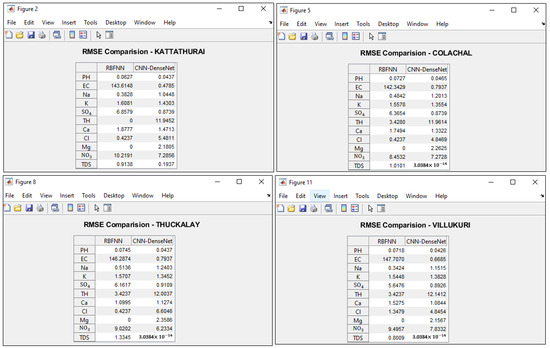
Figure 11.
RMSE comparison.
5.3. Mean Absolute Percentage Error Measure
In the context of the Valliyar Sub-basin, the MAPE was evaluated with independent measures for various regions, namely, Kattathurai, Colachal, Thuckalay, and Villukuri. The assessment depicted in Figure 12 utilized the RBFNN and DenseNet-121 CNN to measure the performance of these classifiers in predicting physiochemical variables. Upon examining the MAPE values for all the observed variables, it is evident that pH predictions benefit from both the RBFNN and DenseNet-121 CNN classifiers, resulting in reduced MAPE values. Specifically, for the area of Kattathurai, the RBFNN classifier yields a MAPE of 0.0123. Similarly, for Colachal, it is 0.0172, for Thuckalay, it is 0.0163, and for Villukuri, the value stands at 0.0146. However, when making a comparative analysis, it becomes apparent that the DenseNet-121 CNN classifier offers improved outcomes. For instance, in case of Kattathurai, the MAPE drops to 0.0079. Similarly, for Colachal, it reduces to 0.0092, for Thuckalay, it improves to 0.0079, and for Villukuri, it reaches 0.0077. The consistent reduction in MAPE values signifies the enhanced capability of the DenseNet-121 CNN model to capture intricate relationships within the data, ultimately resulting in more precise and reliable pH predictions.
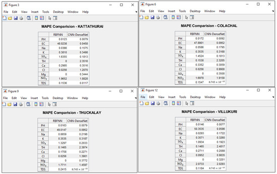
Figure 12.
MAPE comparison.
A comparative analysis was performed in terms of MSE for various parameters, including pH, EC, Ca, Na, K, Cl, TH, and SO4, using machine learning techniques such as ANN [43], SVM [43], DL [43], RBFNN [44] and DenseNet-121 CNN [45], as seen in Figure 13. The findings indicate that the RBFNN and DenseNet-121 CNN techniques yielded the most significant reduction in error. Specifically, when utilizing the RBFNN technique, a pH error of 0.0055 is achieved, and for EC, Ca, Na, K, Cl, TH, and SO4, the values attained are 219.3000, 0.2344, 33.2100, 0.4480, 11.7200, and 33.2140, respectively. In contrast, the DenseNet-121 CNN technique outperformed the other classifiers, resulting in a reduced pH error of 0.0024, an EC error of 0.7210, a Ca error of 3.6400, a Na error of 2.0100, a K error of 0.7800, a Cl error of 20.7700, a TH error of 6.9800, and a SO4 error of 0.7802. It is noteworthy that the DenseNet-121 CNN model achieved the lowest error value for pH, demonstrating its superior performance in the analysis of water quality assessment.
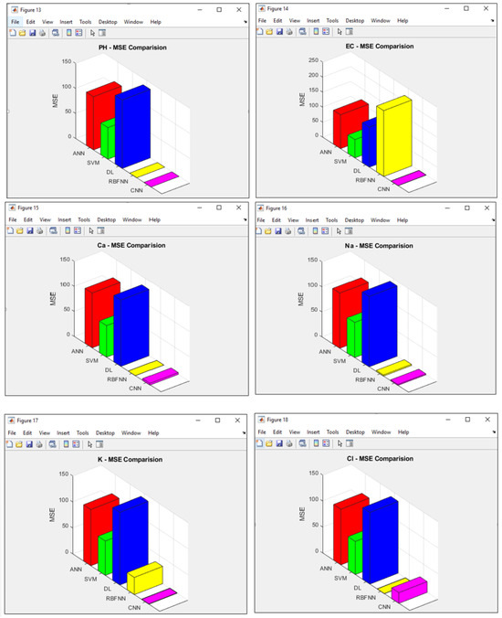
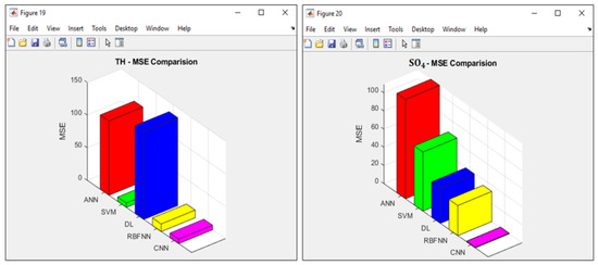
Figure 13.
Comparison of MSE with machine learning techniques.
A comprehensive assessment for RMSE was conducted for a range of parameters, including pH, EC, Ca, Na, K, Cl, TH, and SO4, as shown in Figure 14. The performance evaluation was carried out among various machine learning techniques, specifically the ANN, SVM, DL, RBFNN and DenseNet-121 CNN. The findings consistently pointed to the RBFNN and DenseNet-121 CNN techniques as standout performers in terms of error reduction. While employing the RBFNN technique, an RMSE of 0.0741 for pH was achieved. Additionally, for EC, Ca, Na, K, Cl, TH, and SO4, the RMSE values were calculated at 4.3500, 1.5430, 0.4842, 1.5490, 6.6990, 3.4230, and 5.7632, respectively. In comparison, the DenseNet-121 CNN technique exhibited superior performance, resulting in an RMSE of 0.0487 for pH. Furthermore, the RMSE values obtained for EC, Ca, Na, K, Cl, TH, and SO4 were 0.8490, 1.9100, 1.9100, 1.4181, 4.5570, 8.3560, and 0.8833, respectively. From the analysis it is worth emphasizing that the DenseNet-121 CNN model steadily outperformed the other classifiers by achieving the lowest RMSE value for pH.
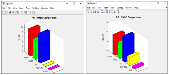
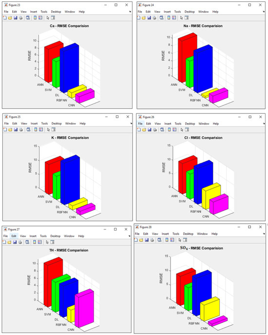
Figure 14.
Comparison of RMSE with machine learning techniques.
A comprehensive analysis was performed using machine learning methods, which included the ANN, SVM, DL, RBFNN and DenseNet-121 CNN. This analysis focused on evaluating the MAPE for various parameters, such as pH, EC, Ca, Na, K, Cl, TH, and SO4, as seen in Figure 15. On analysis, it was revealed that both the RBFNN and DenseNet-121 CNN techniques constantly outperformed the other approaches by delivering highly accurate results with minimal error. For the RBFNN method, a pH error value of 0.0173 was obtained. In addition, for EC, Ca, Na, K, Cl, TH, and SO4, the MAPE values were 47.6200, 0.3022, 0.5860, 0.3510, 0.6410, 1.4650, and 1.2030, respectively. Specifically, a remarkable reduction in MAPE was accomplished by the DenseNet-121 Model, resulting in a pH error of just 0.0099. Furthermore, the MAPE values for EC, Ca, Na, K, Cl, TH, and SO4 were notably low at 0.1136, 0.2380, 0.2930, 0.3480, 0.8736, 1.4432, and 0.1868, respectively. Hence, it is concluded that the DenseNet-121 CNN model consistently outperformed the other classifiers, demonstrating its exceptional accuracy and reliability in the field of water quality assessment.
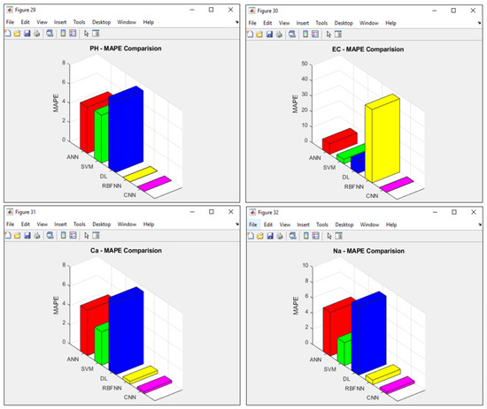
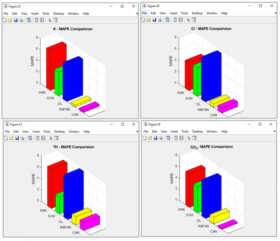
Figure 15.
Comparative analysis of MAPE with machine learning techniques.
The analysis involved assessing the accuracy of predictions for several parameters, for the years spanning from 2019 to 2040. The predictions, using the RBFNN technique and the corresponding results obtained, are visually presented in Figure 16. One notable trend observed in the data was a consistent and linear increase in pH values from the year 2019 to 2040. This means that there is a clear and steady rise in pH levels over this time period. However, for the other parameters, the situation was more complex. These parameters exhibited a combination of rising and falling trends in their values over the same period. These fluctuations suggest that factors influencing these parameters have varying impacts across different years, leading to periodic increases and decreases in their predicted values. Similarly, as shown in Figure 17, the predictions were performed using the DenseNet-121 CNN technique. From 2019 to 2040, the pH values exhibited a clear and linear increase. This indicates that the DenseNet-121 CNN classifier results in steady and continuous rise in pH levels over this extended time frame. In contrast, the behaviours of other parameters are more intricate and dynamic. The fluctuations imply that the factors influencing these parameters exert varying impacts from year to year, resulting in periodic increases and decreases in their predicted values. It is significant that on comparison, the DenseNet-121 CNN method consistently outperformed the RBFNN approach. This underscores the effectiveness of the DenseNet-121 CNN technique in capturing and predicting complex patterns in water quality data over the years.
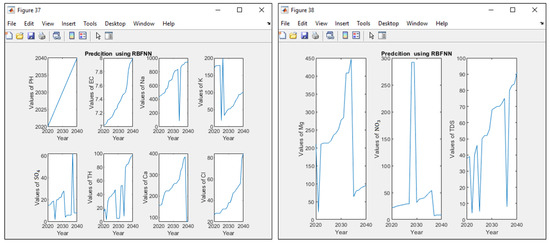
Figure 16.
Prediction using RBFNN technique.
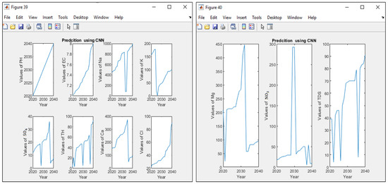
Figure 17.
Prediction using DenseNet-121 CNN technique.
6. Conclusions
In this research work, the predictive analysis of Valliyar Basin’s water quality for the years 2019–2040, with two prominent machine learning models, the RBFNN and DenseNet-121 CNN, was proposed. The variable “Year “acted as a chronological marker, highlighting the long-term trends affecting water parameters. The independent variable significantly impacted the chemical reactions in water, with temperature variations for instance, with mineral solubility and changes in patterns of rainfall influencing the dilution and concentration of the water. The key findings of the research demonstrate that the predictive accuracy of RBFNN is dominated by the DenseNet-121 CNN model’s ability to capture the intricate relations in data. The DenseNet-121 CNN not only generates more accurate forecasts of dependent variable concentrations but also excels in identifying delicate shifts in trends over the years. The pH values obtained through the utilization of the DenseNet-121 CNN model, measured in terms of MSE, showcase remarkable performance across the geographical areas of Kattathurai, Colachal, Thuckalay, and Villukuri, registering values of 0.0019, 0.0022, 0.0019, and 0.0018, respectively. Similarly, the RMSE metrics revealed corresponding values of 0.0437 for Kattathurai, 0.0465 for Colachal, 0.0437 for Thuckalay, and 0.0426 for Villukuri. Moreover, the MAPE values further reinforce the precision of these predictions, demonstrating outstanding results with values of 0.0079 for Kattathurai, 0.0092 for Colachal, 0.0079 for Thuckalay, and 0.0077 for Villukuri. The defined water quality assessment technique not only enabled sustainable water management, but also offered information for decision-makers. Future research focusing on incorporating more diverse environmental parameters and exploring the integration of an advanced technique to enhance the model’s predictive accuracy further. More details of table data can be found in Supplementary Materials.
Supplementary Materials
The following supporting information can be downloaded at: https://www.mdpi.com/article/10.3390/w16111531/s1, Table S1: illustrates the comparison of overall error measures for RBFNN and DenseNet-121 classifiers for the four sub-regions; Table S2: Prediction Result Using RBFNN Classifier for Kattathurai; Table S3: Prediction Result Using RBFNN Classifier for Colachal; Table S4: Prediction Result Using RBFNN Classifier for Thuckalay; Table S5: Prediction Result Using RBFNN Classifier for Villukuri; Table S6: Prediction Result Using DenseNet-121 CNN Classifier for Kattathurai; Table S7: Prediction Result Using DenseNet-121 CNN Classifier for Colachal; Table S8: Prediction Result Using DenseNet-121 CNN Classifier for Thuckalay; Table S9: Prediction Result Using DenseNet-121 CNN Classifier for Villukuri.
Author Contributions
Conceptualization: B.K.R.; data curation: B.K.R.; methodology: S.V. and B.K.R.; project administration: S.V.; supervision: S.V.; validation: S.V.; writing—original draft: B.K.R.; writing—review and editing: S.V. and B.K.R. All authors have read and agreed to the published version of the manuscript.
Funding
The authors received no specific funding for this study.
Data Availability Statement
Data are contained within the article.
Conflicts of Interest
The authors have no conflicts of interest to declare that are relevant to the content of this article.
Abbreviations and Symbols
| Abbreviations | Definition | Symbols | Definition |
| RBFNN | Radial Bias Function Neural Network | Top three leading wolves | |
| CNN | Convolutional Neural Network | Remaining wolves in pack | |
| MSE | Mean-Square Error | Distance vector of | |
| RMSE | Root-Mean-Square Error | Updated Positions of | |
| MAPE | Mean Absolute Percentage Error | Co-efficient Vectors | |
| ANN | Artificial Neural Network | Next position of wolf being updated | |
| SVM | Support Vector Machine | Fixed vector | |
| DL | Deep Learning | Width | |
| VOCs | Volatile Organic Compounds | Gaussian Function | |
| PAHs | Polycyclic Aromatic Hydrocarbons | Weights | |
| pH | Potential Hydrogen | Discrete value | |
| EC | Electrical Conductivity | Actual target value | |
| TDS | Total Dissolved Solids | Loss Function | |
| EPA | Environmental Protection Agency | Concatenated set of feature maps | |
| WHO | World Health Organization | Total input layer channels | |
| KNN | K-Nearest Neighbours | Output layer | |
| PCA | Principal Component Analysis | Base value | |
| TH | Total Hardness | Filter connection with feature map | |
| Na | Sodium | Output layer with features | |
| K | Potassium | Neural network parameter | |
| SO4 | Sulphate | Altering data transformations | |
| Ca | Calcium | RELU layer | |
| Cl | Chloride | Output Layer | |
| Mg | Magnesium | FC layer | |
| NO3 | Nitrate | Weight vector of dimension | |
| GA | Genetic Algorithm | Training Samples | |
| GWO | Grey Wolf Optimization | ||
| FC | Fully Connected | ||
| ReLU | Rectified Linear Unit |
References
- Mosavi, A.; Hosseini, F.S.; Choubin, B.; Goodarzi, M.; Dineva, A.A. Groundwater salinity susceptibility mapping using classifier ensemble and Bayesian machine learning models. IEEE Access 2020, 8, 145564–145576. [Google Scholar] [CrossRef]
- Khan, Q.W.; Kim, B.W.; Ahmed, R.; Rizwan, A.; Khan, A.N.; Kim, K.; Kim, D.H. Predictive Modeling of Water Table Depth, Drilling Duration, and Soil Layer Classification using Adaptive Ensemble Learning for Cost-Effective Percussion Water Borehole Drilling. IEEE Access 2023, 11, 76703–76721. [Google Scholar] [CrossRef]
- Manjakkal, L.; Mitra, S.; Petillot, Y.R.; Shutler, J.; Scott, E.M.; Willander, M.; Dahiya, R. Connected sensors, innovative sensor deployment, and intelligent data analysis for online water quality monitoring. IEEE Internet Things J. 2021, 8, 13805–13824. [Google Scholar] [CrossRef]
- Al-Sulttani, A.O.; Al-Mukhtar, M.; Roomi, A.B.; Farooque, A.A.; Khedher, K.M.; Yaseen, Z.M. Proposition of new ensemble data-intelligence models for surface water quality prediction. IEEE Access 2021, 9, 108527–108541. [Google Scholar] [CrossRef]
- Vivone, G.; Dalla Mura, M.; Garzelli, A.; Pacifici, F. A benchmarking protocol for pansharpening: Dataset, preprocessing, and quality assessment. IEEE J. Sel. Top. Appl. Earth Obs. Remote Sens. 2021, 14, 6102–6118. [Google Scholar] [CrossRef]
- Ram, A.; Tiwari, S.K.; Pandey, H.K.; Chaurasia, A.K.; Singh, S.; Singh, Y.V. Groundwater quality assessment using water quality index (WQI) under GIS framework. Appl. Water Sci. 2021, 11, 1–20. [Google Scholar] [CrossRef]
- Prasad, M.; Sunitha, V.; Reddy, Y.S.; Suvarna, B.; Reddy, B.M.; Reddy, M.R. Data on water quality index development for groundwater quality assessment from Obulavaripalli Mandal, YSR district, AP India. Data Brief 2019, 24, 103846. [Google Scholar] [CrossRef] [PubMed]
- Asadi, E.; Isazadeh, M.; Samadianfard, S.; Ramli, M.F.; Mosavi, A.; Nabipour, N.; Shamshirband, S.; Hajnal, E.; Chau, K.W. Groundwater quality assessment for sustainable drinking and irrigation. Sustainability 2019, 12, 177. [Google Scholar] [CrossRef]
- Lei, R.; Sun, Y.; Zhu, S.; Jia, T.; He, Y.; Deng, J.; Liu, W. Investigation on distribution and risk assessment of volatile organic compounds in surface water, sediment, and soil in a chemical industrial park and adjacent area. Molecules 2021, 26, 5988. [Google Scholar] [CrossRef]
- Halfadji, A.; Touabet, A.; Portet-Koltalo, F.; Derf, F.L.; Merlet-Machour, N. Concentrations and source identification of polycyclic aromatic hydrocarbons (PAHs) and polychlorinated biphenyls (PCBs) in agricultural, urban/residential, and industrial soils, east of Oran (Northwest Algeria). Polycycl. Aromat. Compd. 2020, 39, 299–310. [Google Scholar] [CrossRef]
- Rezaei, A.; Hassani, H.; Jabbari, N. Evaluation of groundwater quality and assessment of pollution indices for heavy metals in North of Isfahan Province, Iran. Sustain. Water Resour. Manag. 2019, 5, 491–512. [Google Scholar] [CrossRef]
- Hasan, M.F.; Nur-E-Alam, M.; Salam, M.A.; Rahman, H.; Paul, S.C.; Rak, A.E.; Ambade, B.; Towfiqul Islam, A.R. Health risk and water quality assessment of surface water in an urban river of Bangladesh. Sustainability 2021, 13, 6832. [Google Scholar] [CrossRef]
- De Jesus, K.L.; Senoro, D.B.; Dela Cruz, J.C.; Chan, E.B. Neuro-particle swarm optimization based in-situ prediction model for heavy metals concentration in groundwater and surface water. Toxics 2022, 10, 95. [Google Scholar] [CrossRef] [PubMed]
- Qi, C.; Huang, S.; Wang, X. Monitoring water quality parameters of Taihu Lake based on remote sensing images and LSTM-RNN. IEEE Access 2020, 8, 188068–188081. [Google Scholar] [CrossRef]
- Wong, W.Y.; Al-Ani, A.K.; Hasikin, K.; Khairuddin, A.S.; Razak, S.A.; Hizaddin, H.F.; Mokhtar, M.I.; Azizan, M.M. Water, soil and air pollutants’ interaction on mangrove ecosystem and corresponding artificial intelligence techniques used in decision support systems-a review. IEEE Access 2021, 9, 105532–105563. [Google Scholar] [CrossRef]
- Ajayi, O.O.; Bagula, A.B.; Maluleke, H.C.; Gaffoor, Z.; Jovanovic, N.; Pietersen, K.C. Waternet: A network for monitoring and assessing water quality for drinking and irrigation purposes. IEEE Access 2022, 10, 48318–48337. [Google Scholar] [CrossRef]
- Gambín, Á.F.; Angelats, E.; González, J.S.; Miozzo, M.; Dini, P. Sustainable marine ecosystems: Deep learning for water quality assessment and forecasting. IEEE Access 2021, 9, 121344–121365. [Google Scholar] [CrossRef]
- Aslam, B.; Maqsoom, A.; Cheema, A.H.; Ullah, F.; Alharbi, A.; Imran, M. Water quality management using hybrid machine learning and data mining algorithms: An indexing approach. IEEE Access 2022, 10, 119692–119705. [Google Scholar] [CrossRef]
- Agrawal, P.; Sinha, A.; Kumar, S.; Agarwal, A.; Banerjee, A.; Villuri, V.G.; Annavarapu, C.S.; Dwivedi, R.; Dera, V.V.; Sinha, J.; et al. Exploring artificial intelligence techniques for groundwater quality assessment. Water 2021, 13, 1172. [Google Scholar] [CrossRef]
- Mohammed, M.A.A.; Khleel, N.A.A.; Szabó, N.P.; Szűcs, P. Modeling of groundwater quality index by using artificial intelligence algorithms in northern Khartoum State, Sudan. Model. Earth Syst. Environ. 2023, 9, 2501–2516. [Google Scholar] [CrossRef]
- Kouadri, S.; Pande, C.B.; Panneerselvam, B.; Moharir, K.N.; Elbeltagi, A. Prediction of irrigation groundwater quality parameters using ANN, LSTM, and MLR models. Environ. Sci. Pollut. Res. 2022, 29, 21067–21091. [Google Scholar] [CrossRef]
- Norouzi, H.; Moghaddam, A.A. Groundwater quality assessment using random forest method based on groundwater quality indices (case study: Miandoab plain aquifer, NW of Iran). Arab. J. Geosci. 2020, 13, 1–13. [Google Scholar] [CrossRef]
- Costache, R. Flash-flood Potential Index mapping using weights of evidence, decision Trees models and their novel hybrid integration. Stoch. Environ. Res. Risk Assess. 2019, 33, 1375–1402. [Google Scholar] [CrossRef]
- Rizwan, A.; Iqbal, N.; Khan, A.N.; Ahmad, R.; Kim, D.H. Toward effective pattern recognition based on enhanced weighted K-mean clustering algorithm for groundwater resource planning in point cloud. IEEE Access 2021, 9, 130154–130169. [Google Scholar] [CrossRef]
- Taşan, M.; Demir, Y.; Taşan, S. Groundwater quality assessment using principal component analysis and hierarchical cluster analysis in Alaçam, Turkey. Water Supply 2022, 22, 3431–3447. [Google Scholar] [CrossRef]
- Shao, C. Data classification by quantum radial-basis-function networks. Phys. Rev. 2020, 102, 042418. [Google Scholar] [CrossRef]
- Hiremath, G.; Mathew, J.A.; Boraiah, N.K. Hybrid Statistical and Texture Features with DenseNet 121 for Breast Cancer Classification. Int. J. Intell. Eng. Syst. 2023, 16, 24–34. [Google Scholar] [CrossRef]
- Wang, S.; Song, X.; Wang, Q.; Xiao, G.; Wang, Z.; Liu, X.; Wang, P. Shallow groundwater dynamics and origin of salinity at two sites in salinated and water-deficient region of North China Plain, China. Environ. Earth Sci. 2012, 66, 729–739. [Google Scholar] [CrossRef]
- Sarkar, S.; Mukherjee, A.; Senapati, B.; Duttagupta, S. Predicting potential climate change impacts on groundwater nitrate pollution and risk in an intensely cultivated area of South Asia. ACS Environ. Au 2022, 2, 556–576. [Google Scholar] [CrossRef]
- Lasagna, M.; Ducci, D.; Sellerino, M.; Mancini, S.; De Luca, D.A. Meteorological variability and groundwater quality: Exam-ples in different hydrogeological settings. Water 2020, 12, 1297. [Google Scholar] [CrossRef]
- Mohammed, L.R.; Kai, K.H.; Kijazi, A.L.; Bakar, S.S.; Khamis, S.A. The Influence of Weather and Climate Variability on Groundwater Quality in Zanzibar. Atmos. Clim. Sci. 2022, 12, 613–634. [Google Scholar] [CrossRef]
- Soumya, B.S.; Sekhar, M.; Riotte, J.; Braun, J.J. Non-linear regression model for spatial variation in precipitation chemistry for South India. Atmos. Environ. 2009, 43, 1147–1152. [Google Scholar] [CrossRef]
- Manzoni, S.; Maneas, G.; Scaini, A.; Psiloglou, B.E.; Destouni, G.; Lyon, S.W. Understanding coastal wetland conditions and futures by closing their hydrologic balance: The case of the Gialova lagoon, Greece. Hydrol. Earth Syst. Sci. 2020, 24, 3557–3571. [Google Scholar] [CrossRef]
- Wu, W.Y.; Lo, M.H.; Wada, Y.; Famiglietti, J.S.; Reager, J.T.; Yeh, P.J.F.; Ducharne, A.; Yang, Z.L. Divergent effects of climate change on future groundwater availability in key mid-latitude aquifers. Nat. Commun. 2020, 11, 3710. [Google Scholar] [CrossRef] [PubMed]
- Kulabako, N.R.; Nalubega, M.; Thunvik, P. Study of the impact of land use and hydrogeological settings on the shallow groundwater quality in a peri-urban area of Kampala, Uganda. Sci. Total Environ. 2007, 381, 180–199. [Google Scholar] [CrossRef] [PubMed]
- Brindha, K.; Neena Vaman, K.V.; Srinivasan, K.; Sathis Babu, M.; Elango, L. Identification of surface water-groundwater interaction by hydrogeochemical indicators and assessing its suitability for drinking and irrigational purposes in Chennai, Southern India. Appl. Water Sci. 2014, 4, 159–174. [Google Scholar] [CrossRef]
- Thivya, C.; Chidambaram, S.; Thilagavathi, R.; Ganesh, N.; Panda, B.; Prasanna, M.V. Short-term periodic observation of the relationship of climate variables to groundwater quality along the KT boundary. J. Clim. Chang. 2018, 4, 77–86. [Google Scholar] [CrossRef]
- Rajendiran, T.; Sabarathinam, C.; Chandrasekar, T.; Keesari, T.; Senapathi, V.; Sivaraman, P.; Viswanathan, P.M.; Nagappan, G. Influence of variations in rainfall pattern on the hydrogeochemistry of coastal groundwater—An outcome of periodic observation. Environ. Sci. Pollut. Res. 2019, 26, 29173–29190. [Google Scholar] [CrossRef] [PubMed]
- Adham, A.K.M.; Kobayashi, A.; Murakami, A. Effect of climatic change on groundwater quality around the subsurface dam. Geomate J. 2011, 1, 25–31. [Google Scholar]
- Kløve, B.; Ala-Aho, P.; Bertrand, G.; Gurdak, J.J.; Kupfersberger, H.; Kværner, J.; Muotka, T.; Mykrä, H.; Preda, E.; Rossi, P.; et al. Climate change impacts on groundwater and dependent ecosystems. J. Hydrol. 2014, 518, 250–266. [Google Scholar] [CrossRef]
- Saito, T.; Hamamoto, S.; Ueki, T.; Ohkubo, S.; Moldrup, P.; Kawamoto, K.; Komatsu, T. Temperature change affected groundwater quality in a confined marine aquifer during long-term heating and cooling. Water Res. 2016, 94, 120–127. [Google Scholar] [CrossRef] [PubMed]
- Hassanzadeh, R.; Komasi, M.; Hassanzadeh, A.; Derikv and, A. Trend Analysis of Groundwater Quality Using Coherence and Cross Wavelet (Case Study of Khorramabad City). J. Civ. Eng. Mater. Appl. 2021, 5, 164–176. [Google Scholar]
- Bhagavathi, K.R.; Sankararajan, V. Prediction and Assessment of Minerals Contamination in Groundwater: Analytical Tools Approach. Indian J. Ecol. 2022, 49, 324–331. [Google Scholar]
- Li, T.; Lu, J.; Wu, J.; Zhang, Z.; Chen, L. Predicting aquaculture water quality using machine learning approaches. Water 2022, 14, 2836. [Google Scholar] [CrossRef]
- Anand, M.V.; Sohitha, C.; Saraswathi, G.N.; Lavanya, G.V. Water quality prediction using CNN. In Journal of Physics: Conference Series; IOP Publishing: Bristol, UK, 2023; Volume 2484, p. 012051. [Google Scholar]
Disclaimer/Publisher’s Note: The statements, opinions and data contained in all publications are solely those of the individual author(s) and contributor(s) and not of MDPI and/or the editor(s). MDPI and/or the editor(s) disclaim responsibility for any injury to people or property resulting from any ideas, methods, instructions or products referred to in the content. |
© 2024 by the authors. Licensee MDPI, Basel, Switzerland. This article is an open access article distributed under the terms and conditions of the Creative Commons Attribution (CC BY) license (https://creativecommons.org/licenses/by/4.0/).